Synthetic MRI Generation from CT Scans for Stroke Patients

Abstract

CT scans are currently the most common imaging modality used for suspected stroke patients due to their short acquisition time and wide availability. However, MRI offers superior tissue contrast and image quality. In this study, eight deep learning models are developed, trained, and tested using a dataset of 181 CT/MR pairs from stroke patients. The resultant synthetic MRIs generated by these models are compared through a variety of qualitative and quantitative methods. The synthetic MRIs generated by a 3D UNet model consistently demonstrated superior performance across all methods of evaluation. Overall, the generation of synthetic MRIs from CT scans using the methods described in this paper produces realistic MRIs that can guide the registration of CT scans to MRI atlases. The synthetic MRIs enable the segmentation of white matter, grey matter, and cerebrospinal fluid by using algorithms designed for MRIs, exhibiting a high degree of similarity to true MRIs.

1. Introduction

Computed Tomography (CT) and Magnetic Resonance Imaging (MRI) are the most widely used imaging modalities for imaging the brain. Patients who present with suspected stroke most commonly receive a CT scan for initial evaluation due to its lower cost and shorter acquisition time compared to MRI. However, MRI has been shown to be more accurate than CT for diagnosing stroke and can provide additional information that can be useful for the diagnosis, treatment, and prognosis of stroke and other brain disorders. Additionally, MRI can be used to detect other abnormalities in the brain that may contribute to stroke risk, such as aneurysms, arteriovenous malformations, or tumours.

MRI is more sensitive than CT at detecting lesions in conditions such as stroke due to its superior soft tissue contrast and ability to provide detailed anatomical information [1,2,3,4]. Once medical images are obtained, analysis is necessary to facilitate diagnosis. Comparing the patient’s brain scans to a brain atlas can be helpful in understanding the location of lesions or abnormalities with respect to the anatomical and functional structures of the brain. Many commonly used brain atlases, including the MNI152 T1-weighted MRI brain template [5], Talairach atlas [6], Brodmann atlas [7], and JHU DTI-based white-matter atlases [8], are derived from MRI. However, cross-modality image registration between CT and MRI is challenging due to the high variability of tissue and organ appearance caused by the different imaging mechanisms. The pixel intensity, voxel size, image orientation, and field of view are also different between CT and MRI images, making multimodality registration less straightforward than monomodality registration [9].

While MRI is more accurate than CT in diagnosing stroke, not all emergency rooms are equipped with MRI scanners, especially in smaller or poorer areas. In such cases, it may be beneficial to use deep learning techniques to generate a synthetic MRI from the patient’s CT scan. Deep learning techniques are being increasingly applied to various areas of medicine, including stroke diagnosis and treatment. One of the primary uses of deep learning in this field is medical image segmentation, where an algorithm is trained to automatically identify and segment lesions from a brain scan. This can help to improve accuracy and efficiency in diagnosis and treatment planning for stroke patients.

Previous studies have primarily focused on MRI to CT generation [10,11,12,13,14,15,16,17,18,19], often for the purpose of MRI-only radiotherapy. A survey of the literature revealed eight papers which have studied CT-to-MRI synthesis [20,21,22,23,24,25,26,27]; these studies are detailed in

Table 1. Related work.

Study	Region of Interest	Number of Patients	Paired	GAN	CNN	Transformers
[20]	Pelvis	17	✓	✓	✓	✗
[21]		140	✓	✓	✗	✗
[22]	Lumbar Spine	285	✓	✓	✗	✗
[23]	Head and Neck	118	✓	✓	✗	✗
[24]		229 *	✗	✓	✗	✗
[25]	Brain	34	✓	✓	✓	✗
[26]		34	✓	✓	✓	✗
[27]		103	✓	✓	✗	✗
Ours		181	✓	✓	✓	✓

* CT scans from 202 Patients and MRIs from 27 different patients.

. Of these, only one study [27] investigated MRI generation for stroke patients, using a dataset of 103 patients and only implementing GANs. In this paper, we use a dataset of 181 patients and implement many different models including CNNs and GANs, using a variety of attention mechanisms including transformers. This is the first study using CNNs for MRI generation for stroke patients and the first study using transformers for CT-to-MRI synthesis. Moreover, this study improves on the previous studies of CT-to-MRI synthesis in the brain by using the largest dataset, adjusting the CNN model architectures from segmentation models to image generation models, comparing an extensive number of state-of-the-art medical image techniques, and comprehensively evaluating the models for their unique application to stroke patients. Finally, we provide code for all of the developed models in an open-source repository [28].

The purpose of this study is to investigate the use of different deep learning algorithms to generate realistic and accurate MRIs of a patient from their CT scan while considering the niche aspects of this problem in translating stroke lesions between the scans. This study uses multiple versions of a UNet model adapted for image synthesis, as well as UNet++ and attention-based UNets, and compares 2D, 3D, and patch-based models. These paired architectures are compared to the unpaired CycleGAN. The results are evaluated, and the performance of the different models is compared by using a combination of qualitative and quantitative methods.

2. Materials and Methods

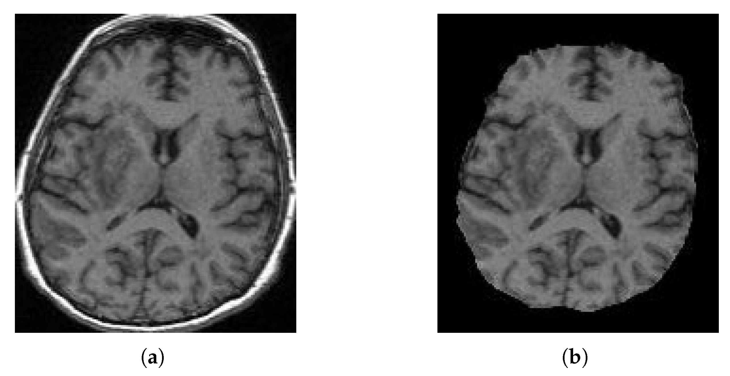
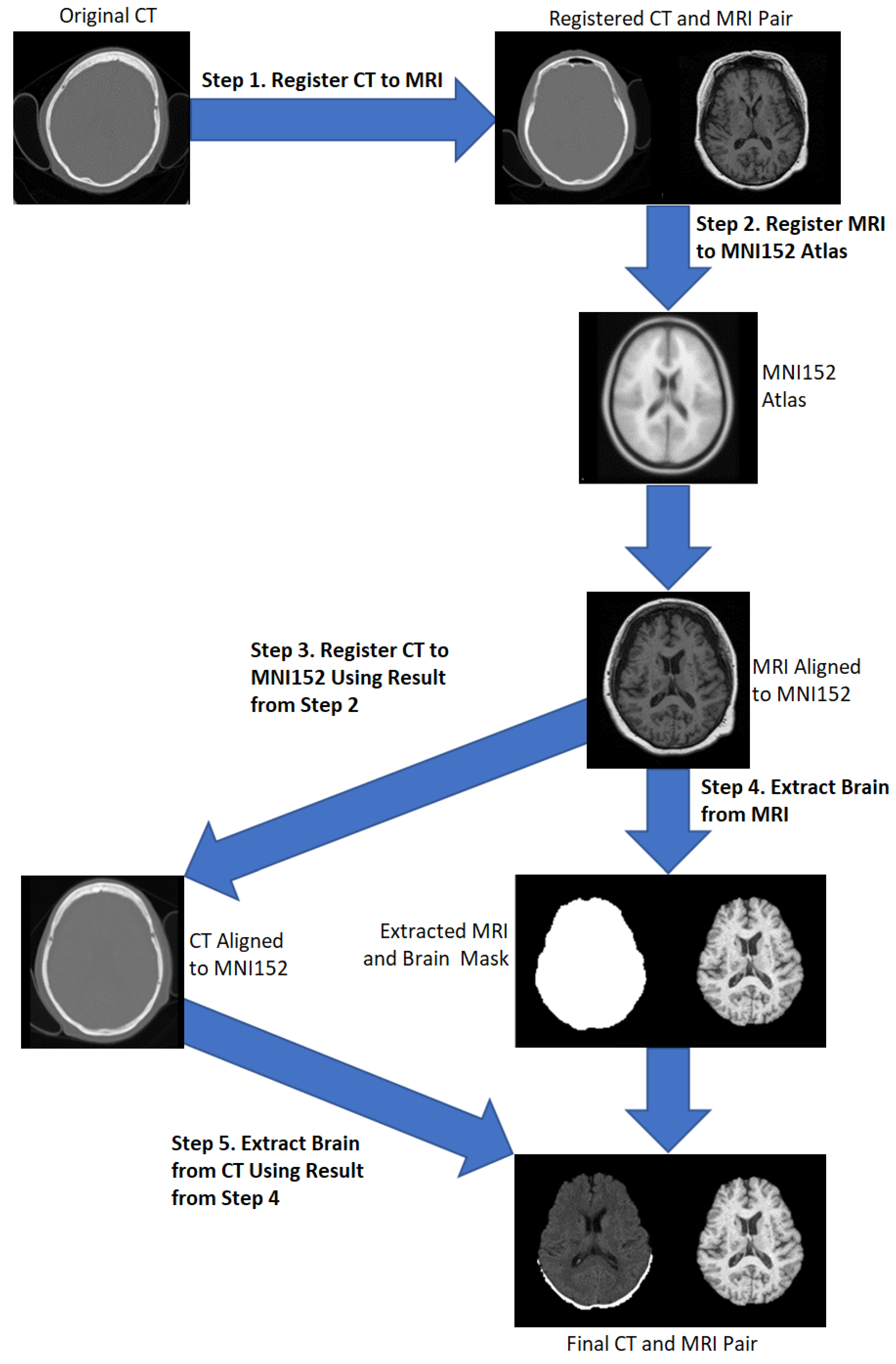
The dataset used in this research consists of 181 patients who were treated for stroke at Auckland City Hospital between 2009 and 2020. All patients received both a CT and T1-weighted MRI scan, which were available on file. The dataset was formed by combining multiple datasets from previous research studies. Each of the patients were required to be at least 18 years old and gave written informed consent. Patients with Ischaemic and Haemorrhagic strokes were included.

The dataset consisted of 89 females and 92 males. The age range was 31–97 years with a mean of 70 years, a median of 71 years, and a standard deviation of 15 years (Figure 1). In total, 18 subjects suffered a Haemorrhagic stroke, and 163 suffered an Ischaemic stroke. A total of 99 patients had a stroke in the right hemisphere and 82 had a stroke in the left hemisphere.

Table 2. MRI acquisition parameters for included studies.

Study	n	Scanner	TR (ms)	TE (ms)	TI (ms)	Flip (∘)	Sequence *
1	55	Avanto 1.5 T	11	4.94	n/a	15	FLASH3D
2	47	Avanto 1.5 T	13	4.76	n/a	25	FLASH3D
3	8	Skyra 3 T	23	2.46	n/a	23	FLASH3D
4	18	Skyra 3 T	1900	2.07	900	9	FLASH3D, MPRAGE
5	53	Avanto 1.5 T	2200	2.97	900	8	FLASH3D, MPRAGE

* n—Sample Size, TR—Repetition Time, TE—Echo Time, TI—Inversion Time, Flip—Flip Angle.

gives the MRI acquisition parameters for the included studies. All MRIs were acquired with a 1.0 × 1.0 × 1.0 mm resolution.

2.1. Preprocessing

A pipeline was developed to preprocess the data, which included registration to a brain atlas and brain extraction. The following steps detail the preprocessing pipeline (Figure 2):

• Registration of the CT to the MRI using FSL Flirt [29,30,31] with 12 degrees of freedom and a mutual information cost function.
• Registration of the MRI to the ICBM152 T1w linear atlas using FSL Flirt [29,30,31] with 12 degrees of freedom and a correlation ratio cost function, and saving the transformation matrix.
• Applying the transformation matrix from step 2 to the resultant CT from step 1.
• Apply the runhdbet function of HD-BET [32] to the resultant MRI from step 2. The resultant extraction brain and brain mask are then saved.
• Using pixelwise multiplication between the resultant CT scan from step 3 and the brain mask from step 4 to extract the brain from the CT.

After the data were processed through the pipeline, the data underwent manual quality control by overlaying the CT and MRI of each patient and visually inspecting the alignment over multiple slices. Data that could not be successfully registered from CT to MRI in FSL Flirt were attempted to be registered in 3D Slicer [33,34,35,36]. To ensure consistency between the images, all MRI images were set to a data range of [0, 255] by dividing the intensities of each image by its maximum intensity and multiplying by 255. CT scans were kept in their original intensity range as they were in Hounsfield Units.

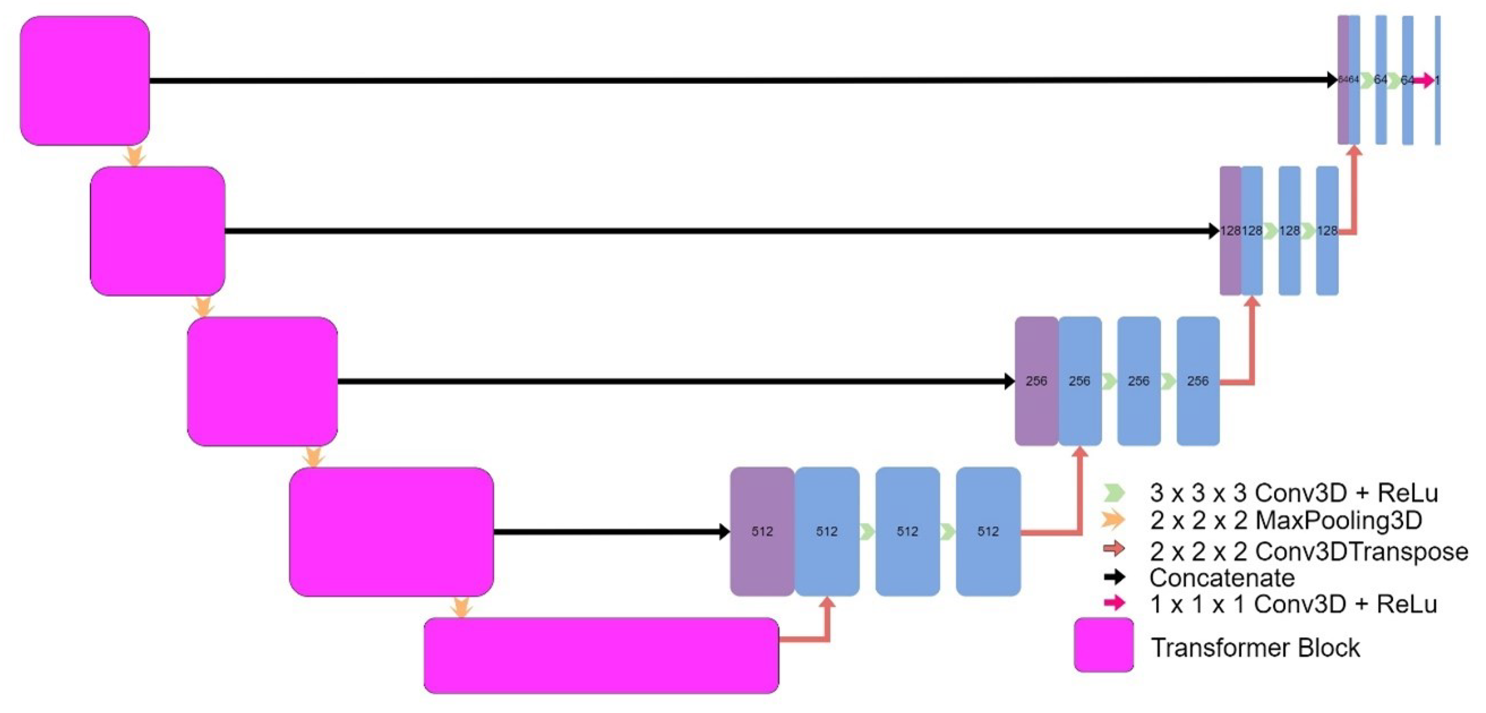
2.2. Model Architectures

Eight models were implemented, including four models based on the original UNet [37]. UNet V1 (Figure 3) is a five-layer 3D UNet which we adjusted to be suitable for image generation and which used convolution transposes as the upsampling operation. We developed 3D UNet V2 (Figure 3), which uses upsampling and convolutions instead of transpose convolutions as it has been demonstrated that this reduces checkerboard artefacts [38]. We developed patch-based UNet (Figure 3) as a variation of UNet V1, which was trained on nonoverlapping patches of the data to reduce memory usage of the model. Similarly, 2D UNet (Figure 4) was developed based on UNet V1 to be trained on full size axial slices.

Three further models based on improved versions of UNet were developed. UNet++ (Figure 5) is a five-layer 3D UNet which we developed based on the UNet++ architecture [39] and adjusted to be suitable for image generation. Attention UNet (Figure 6) is a five-layer 3D UNet with attention blocks in the skip connections which we developed based on the Attention UNet architecture [40] and adjusted to be suitable for image generation. Finally, we introduce our novel implementation of transformers [41] into the encoder of a five-layer 3D UNet model designed for image generation to form Transformer UNet (Figure 7). These three models were developed as patch-based models as the additional parameters made it impossible to train with the full-size data due to memory limitations.

Finally, an implementation of CycleGAN by David Iommi [42] was used to compare the UNet variations to a GAN.

Table 3. Hyperparameters.

Model	Number of Epochs	Learning Rate	Patch Based	Input Dimension	Batch Size	Loss Function	Training Environment
UNet V1	400	$5\times {10}^{-5}$	✗	176 × 192 × 176	1	MAE	1 × 80 GB Tensorflow
UNet V2	400	$5\times {10}^{-5}$	✗	176 × 192 × 176	1	MAE	1 × 80 GB Tensorflow
UNet Patch	400	$5\times {10}^{-5}$	✓	96 × 96 × 96	4	MAE	4 × 32 GB Tensorflow
UNet 2D	400	$5\times {10}^{-5}$	✗	192 × 176	16	MAE	4 × 32 GB Tensorflow
UNet++	400	$5\times {10}^{-5}$	✓	96 × 96 × 96	4	MAE	4 × 32 GB Tensorflow
Attention UNet	400	$5\times {10}^{-5}$	✓	96 × 96 × 96	4	MAE	4 × 32 GB Tensorflow
Transformer UNet	400	$5\times {10}^{-5}$	✓	96 × 96 × 96	1	MAE	1 × 80 GB Tensorflow
CycleGAN	200	$2\times {10}^{-4}$	✓	112 × 112 × 112	6	MAE/BCE *	6 × 32 GB Pytorch

* CycleGAN uses MAE as the loss function to measure the discriminator’s accuracy and BCE for the cycle-consistent component. The total loss function combines these. MAE—Mean Absolute Error, BCE—Binary Cross Entropy.

summarises some of the differences between all the models we utilised. Code for all of the models we have developed is publicly available [28].

2.3. Training and Evaluation

Table 3 summarises the hyperparameters selected for each model and details information about the training environment. The dataset of 181 stroke patients was split into training, validation, and test sets with 144 patients in the training set, 18 patients in the validation set, and 19 patients in the test set. CycleGAN did not use a validation set and instead had the training and validation sets combined to form 162 patients in the training set and 19 patients in the test set. Each model was evaluated on the data from the 19 test subjects. The model was run with CT scans as inputs and the outputs were compared to the true MRIs through quantitative metrics: PSNR, SSIM, MAE, and MSE. The results were visually compared, and the appearance of any lesions was analysed.

The quantitative metrics were calculated only over the voxels within the brain—excluding the background of the image. All voxels within the brain on the true MRIs had a nonzero intensity, while the background was zero everywhere. To compute the evaluation metrics over only the brain, voxels were only included in the calculation if the intensity of the voxel in the true MRI was nonzero.

To ensure that the synthetic MRIs accurately portrayed lesions, we tested if the true lesion(s) in the original MRI were present in the synthetic MRIs. In research settings, lesion segmentation is often performed manually by medical professionals, but many studies have aimed to automate this task by using machine learning; however, this is generally not performed for T1w MRIs at the acute stage. As obtaining a well-trained lesion segmentation model can be challenging, a pretrained model from the ATLAS dataset [43] was used in this study. To assess the performance of the 8 models in generating synthetic MRIs that accurately portrayed lesions, the pretrained segmentation model was applied to the synthetic MRIs generated by each model and the original MRI scans of two patients in the test set.

One of the main advantages of MRIs over CT scans for stroke diagnosis is the higher contrast they provide between different types of tissue. To evaluate the ability of synthetic MRIs to replicate this feature, the tissue segmentation of white matter, grey matter, and cerebral spinal fluid was performed by using FSL FAST [44].

Registration of the CT, synthetic MRI, and true MRI was performed by using the registration module in 3D Slicer to evaluate the usefulness of synthetic MRIs in reducing cross-modal registration to monomodal registration. A randomly selected patient (Patient Alpha) from the training set, whose original MRI was not registered to the MNI152 atlas during the preprocessing, was chosen as the target registration space, as shown in Figure 8. Brain extraction using the SwissSkullStripper module of 3D Slicer was performed on Patient Alpha’s MRI to prepare it for registration. Patient H’s true CT, true MRI, and synthetic MRIs from each of the eight models were individually registered to Patient Alpha’s MRI by using the BRAINS Registration in 3D Slicer, with the transformation matrices and registered volumes saved. All the transforms were applied to one volume to compare registration results without being affected by differences between the synthetic and true MRIs. The CT underwent all nine saved transformations, and the CT transformation matrix from the true MRI was taken to be the optimal registration that all others were compared to. Matte’s Mutual Information (MMI) was calculated by using the BRAINS metrics module in 3D Slicer to compare the nine other transformations.

3. Results

3.1. UNet V1

Figure 9 shows a sample slice of the synthetic MRI generated by 3D UNet for three patients in the test set, along with the corresponding true MRI and CT slices. Patient A presents a large lesion, which can also be seen in the synthesised MRI, but with reduced contrast and less-precise borders. Patient B shows a similar overall contrast to the true MRI. Patient C displays a very large, faint lesion that is not clearly visible in the synthetic MRI.

3.2. UNet V2

Figure 10 shows a slice of the synthetic MRI generated by 3D UNet by using an upsampling layer and a convolution layer instead of the Conv3DTranspose layer. The lesion for Patient A is clearly visible and appears similar in shape to the true MRI. The lesion in Patient C is also discernible, albeit faint and lacking a clear outline. All three synthetic images show good contrast and likeness to the original image.

3.3. Patch-Based UNet

Figure 11 presents the results of a patch-based 3D UNet. The edges of the patches are clearly visible, and the patches do align smoothly but still differ in intensity. The lesion can be clearly seen in the synthetic image for Patient A, appearing on both of the left-hand side patches. It is difficult to tell whether the lesion is present for Patient C, although the general region appears hypointense.

3.4. 2D UNet

Figure 12 shows the results of a 2D UNet trained on the axial slices of the dataset. All three of the synthetic MRIs show a wide range of shades and detail across the brain while maintaining suitable contrast. For Patient A, the lesion is clearly visible with an accurate boundary—however, it is quite faint, and the intensity is not consistent throughout. The synthetic MRI for Patient C does not have a clearly visible lesion, but there appears to be a boundary with a similar shape and size to the true lesion.

3.5. UNet++

Figure 13 shows the results from a 3D patch-based UNet++ model. In the synthesised MRI for Patient A, the intensity varies between patches, making the patch edges very visible and the presence of a lesion uncertain. On the other hand, Patient B’s synthesised MRI presents an excellent and realistic level of contrast and detailing of the grey matter structures. Patient C’s MRI lacks contrast, and the lesion seems to be absent.

3.6. Attention UNet

Figure 14 shows the results of a patch-based UNet with attention gates built into the skip connections. In the synthesised MRI for Patient A, the intensity again varies between the patches, making the patch edges very visible. Patient B displays good contrast; however, some of the grey matter structures are blurry. The lesions do not appear to be present for Patients A and C.

3.7. Transformer UNet

Figure 15 presents the results of a patch-based UNet using transformer blocks in the encoder. In the synthetic MRI for Patient A, the lesion appears extremely dark with a sharp but inaccurate boundary. Patient B’s synthetic MRI displays good contrast and accurately captures many regions of grey matter. In the synthetic MRI for Patient C, the lesion is not clearly visible.

3.8. CycleGAN

Figure 16 shows the results of a 3D CycleGAN [42] run with a patch size of 112 × 112 × 112. The images display very good contrast; however, the shape of the sulci is not always accurate. The lesion for Patient A is faint and there is no lesion visible in Patient C. The images also show a checkerboard pattern.

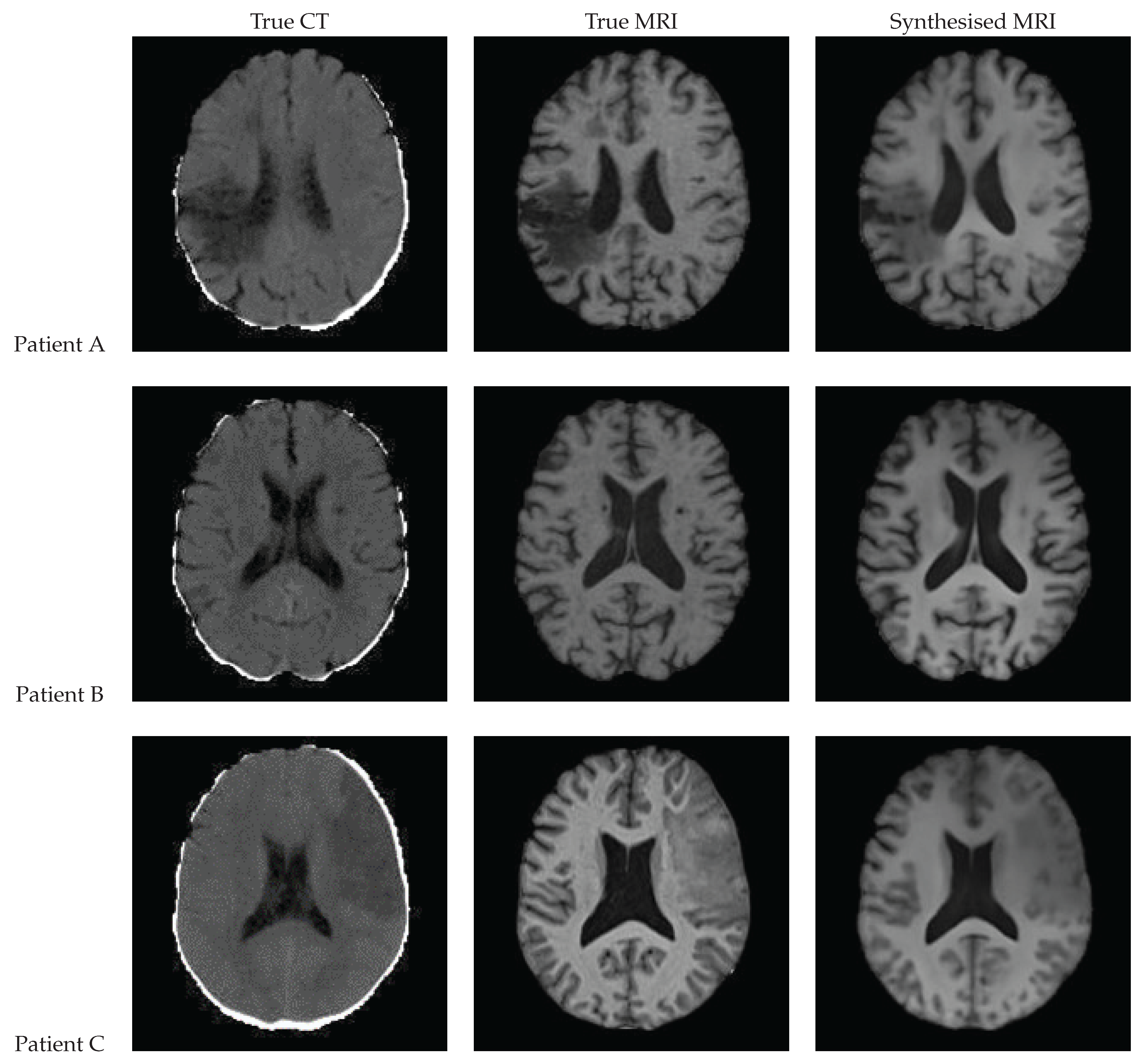
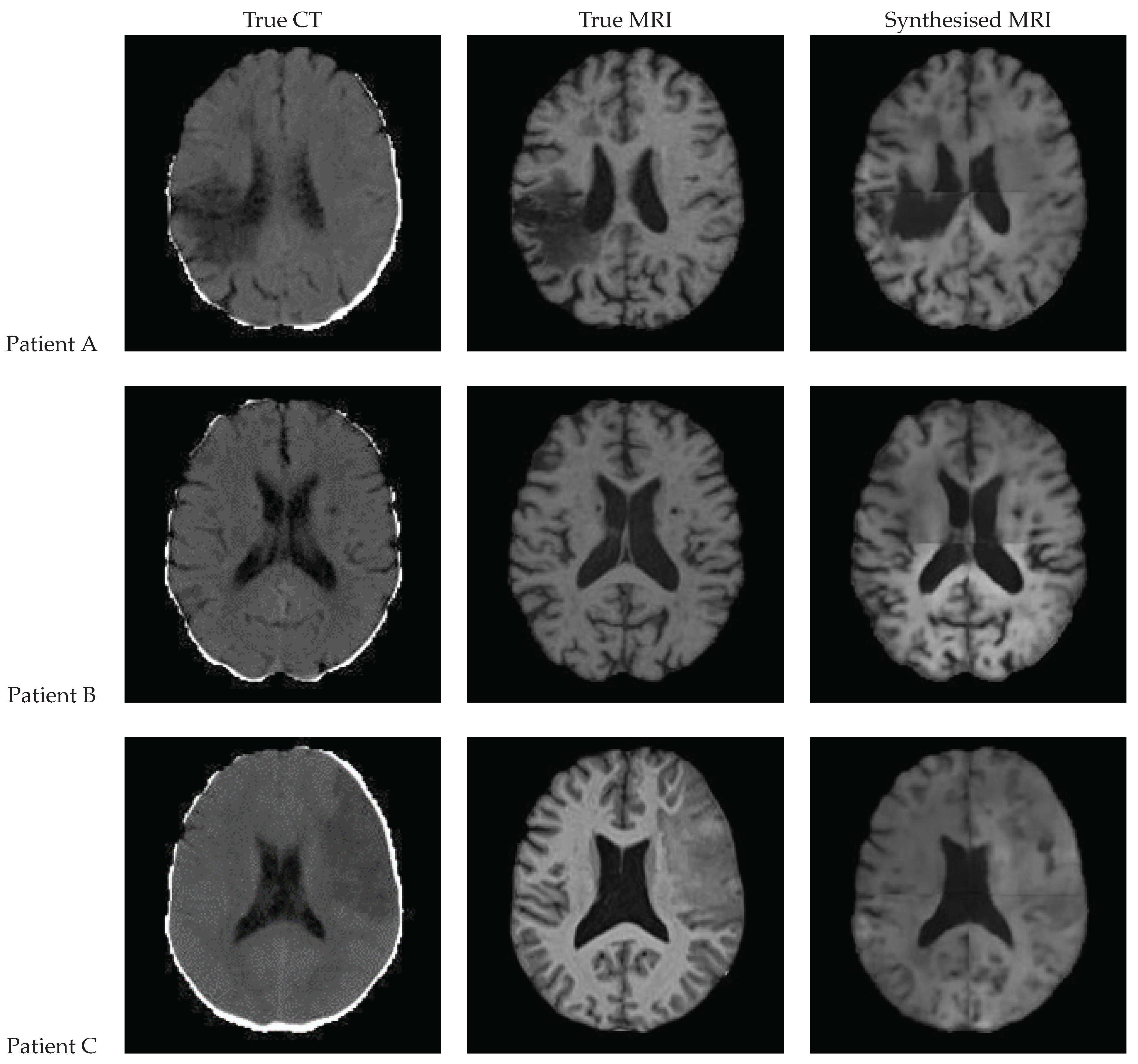
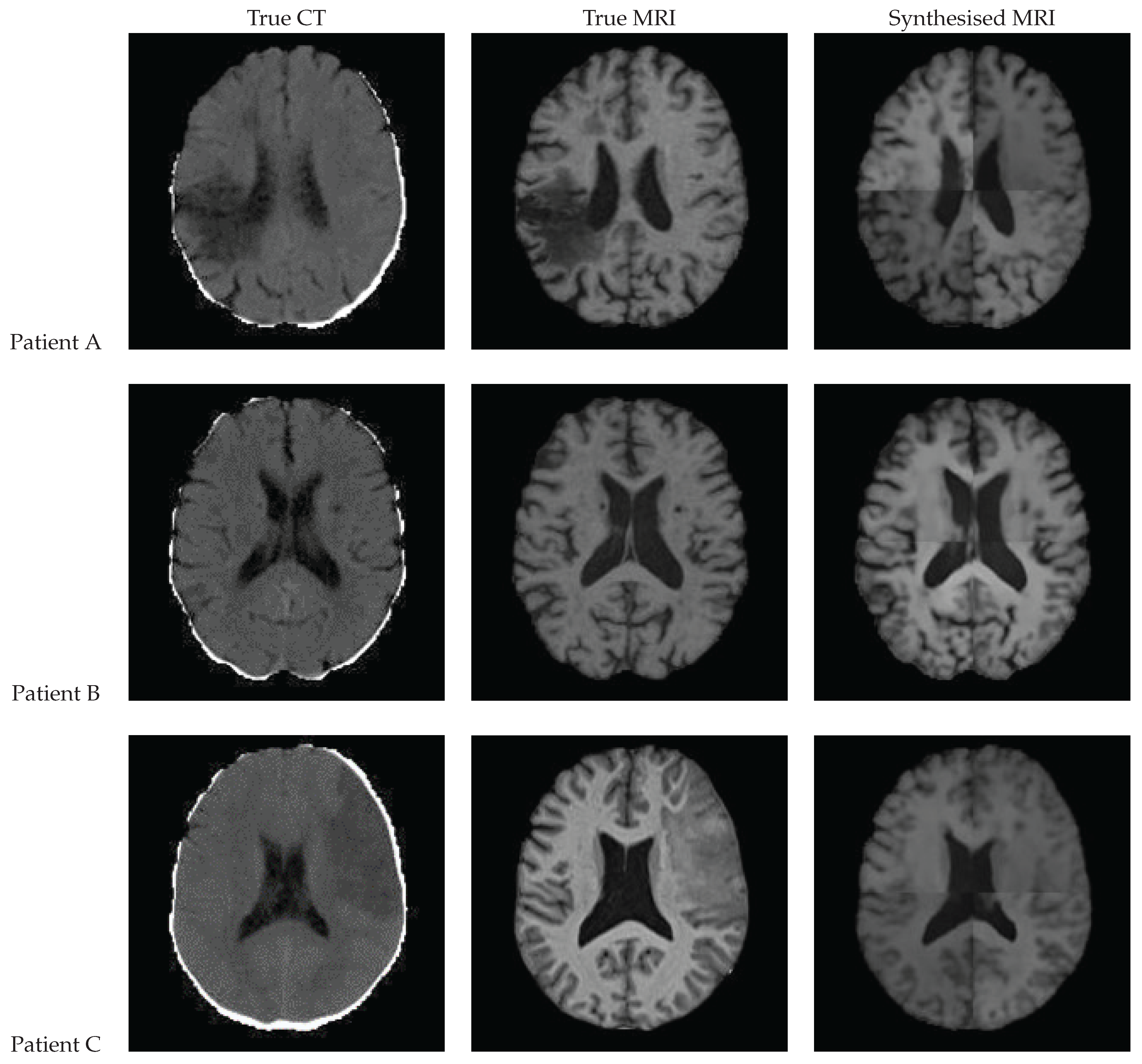
3.9. Qualitative Assessment

All the models except UNet++ and Attention UNet clearly depict the lesion for Patient A; however, most of the lesions in the synthesised MRIs lacked contrast. CycleGAN appeared to have the least contrast between the lesion and surrounding area. Transformer UNet exhibited considerably higher contrast for the lesion; however, it failed to accurately capture the lesion’s boundary. 2D UNet gave rise to a mottled effect over the lesion area.

Patient C presented with a notably large lesion; however, only UNet V2 and 2D UNet managed to retain any indication of the lesion. Nevertheless, the presence of the lesion remains subject to debate in both cases. The models encountered difficulties in accurately reproducing other features of Patient C’s dataset. Additionally, with the exception of CycleGAN, they lacked the necessary contrast between the various types of brain tissue. The inability to generate sufficient contrast was observed across multiple synthetic MRIs, particularly in cases where the true MRI exhibited lower levels of contrast. CycleGAN demonstrated good contrast across all synthetic MRIs; however, it often failed to replicate the brain structures found on the true MRI. Specifically, CycleGAN seemed to have learned the presence of sulci along the brain’s edge but generated them in a semirandom manner rather than reproducing the patterns observed in the CT. The 2D UNet model exhibited notable accuracy in modelling gyri and sulci in the synthesised MRI, displaying good contrast. On the other hand, the patch-based models faced challenges in accurately predicting the edges of the patches, resulting in misalignment issues. Figure 17 shows seven axial slices of the true MRI and the synthetic MRIs from each of the eight models for Patient D.

Patch outlines in the nonoverlapping patch-based models are clearly visible. The inaccurate patch alignments and difference in contrast between the patches stands out, detracting from the contrast of lesions, different tissue types, and other features within the brain. Despite other issues, CycleGAN—which uses overlapping patches—does not suffer from this.

3.10. Quantitative Assessment

Table 4. Evaluation metrics for each model averaged over the test set along with standard deviations. The best result for each metric is shown in bold.

Model	MAE ↓	MSE ↓	SSIM ↑	PSNR ↑	Total SSIM ↑ *
UNet	$\mathbf{18.29}\pm \mathbf{6.61}$	$\mathbf{558.93}\pm \mathbf{405.03}$	$\mathbf{0.687}\pm \mathbf{0.071}$	$\mathbf{21.571}\pm \mathbf{2.724}$	$\mathbf{0.882}\pm \mathbf{0.030}$
UNet V2	$20.23\pm 7.29$	$671.03\pm 463.26$	$0.676\pm 0.062$	$20.659\pm 2.483$	$0.877\pm 0.028$
2D UNet	$19.23\pm 7.20$	$615.40\pm 509.75$	$0.613\pm 0.063$	$21.097\pm 2.491$	$0.834\pm 0.029$
Patch-Based UNet	$19.18\pm 8.00$	$632.61\pm 557.50$	$0.649\pm 0.071$	$21.176\pm 2.763$	$0.867\pm 0.031$
Attention UNet	$19.50\pm 7.77$	$653.92\pm 561.15$	$0.642\pm 0.068$	$20.964\pm 2.648$	$0.865\pm 0.030$
UNet++	$20.28\pm 8.42$	$683.76\pm 562.59$	$0.657\pm 0.067$	$20.800\pm 2.751$	$0.870\pm 0.029$
Transformer UNet	$19.44\pm 7.56$	$651.78\pm 595.69$	$0.645\pm 0.077$	$23.990\pm 2.665$	$0.865\pm 0.034$
CycleGAN	$23.55\pm 10.57$	$978.71\pm 1075.83$	$0.467\pm 0.083$	$19.345\pm 2.591$	$0.780\pm 0.040$

* Total SSIM is calculated over the entire volume. All other metrics are calculated over the voxels within the brain.

shows the four common image evaluation metrics (MAE, MSE, PSNR, and SSIM) calculated between the synthetic MRIs and true MRIs averaged over the 19 patients in the test set. Only the voxels in the brain were used to compute these metrics due to the complexities of calculating the SSIM over only the brain voxels. The total SSIM (calculated over the entire volume) is also listed. UNet achieved the best scores across all metrics, while CycleGAN achieved the worst scores across all metrics.

3.11. Performance at Clinically Relevant Tasks

3.11.1. Registration

Figure 18 displays the resulting registrations for each MRI and the corresponding CT in the first column, along with the CT that underwent the associated transformation in the second column. The mutual information between the presented CT and the CT which underwent the true MRI transformation is provided for each case. All of the synthetic MRIs achieved a suitable alignment to the target MRI, determined by a qualitative analysis of the guided CT alignments and the mutual information scores. In contrast, the unguided CT scans were not aligned accurately and required significantly more time when calculating the transformation.

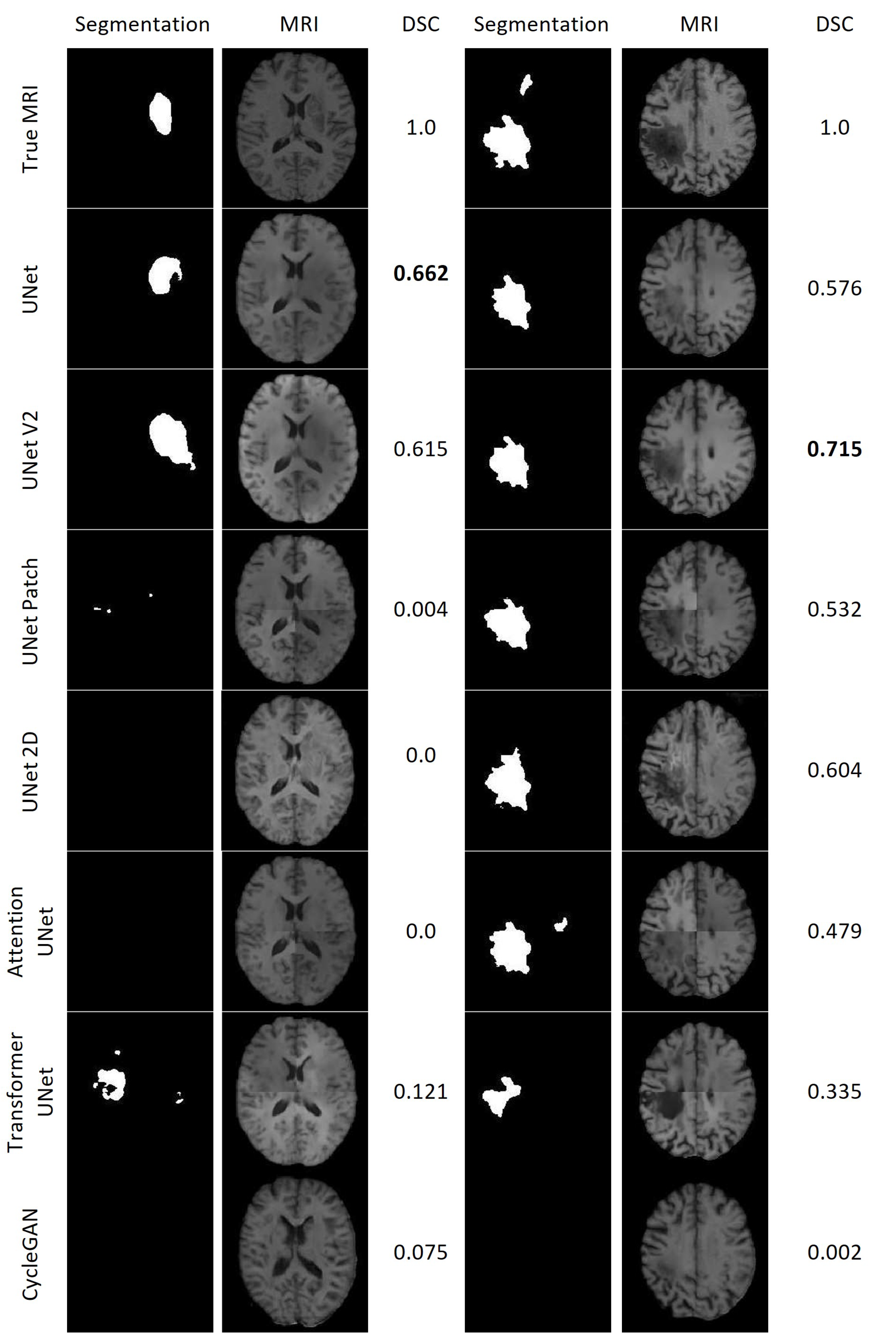
3.11.2. Lesion Segmentation

Figure 19 displays the results of the lesion segmentation algorithm applied to the synthetic and true MRIs of two patients within the test set. Patient E exhibited a smaller lesion that lacked significant contrast in any of the synthetic MRIs. Among the synthetic MRIs, only those generated by UNet and UNet V2 produced lesion segmentations resembling the original MRI for Patient E, with Dice Scores (DSC) of 0.662 and 0.615, respectively. The next best performing model was Transformer UNet, achieving a DSC of 0.121. For Patient A, all synthetic MRIs, except those generated by CycleGAN, yielded lesion segmentations resembling the true MRI. The most accurate lesion segmentation for Patient E was obtained from the UNet V2 synthetic MRI, with a DSC of 0.715.

3.11.3. Brain Tissue Segmentation

Figure 20 displays the results of the FAST algorithm applied to each MRI synthesis model and the true MRI for two patients. FAST did not perform well when applied to the CycleGAN results. Interestingly, the output classified most voxels as cerebrospinal fluid (CSF) for both patients, despite and unknown reason for this behaviour. Furthermore, in the patch-based models, it is evident that the FAST algorithm struggles to classify the regions around the edges of the patches. In the case of the 2D UNet synthetic MRI, the FAST model fails to identify CSF around the edge of the brain and instead misclassifies some areas outside the brain as CSF. Overall, UNet and UNet V2 demonstrate the best performance. UNet achieved the highest DSC for the GM and WM for Patient F, as well as the best WM DSC for Patient G. On the other hand, UNet V2 achieved the best WM DSC for Patient F and the best GM DSC for patient G. UNet++ attained the highest DSC CSF score for Patient G.

4. Discussion

This study evaluated the synthetic MRIs generated from CT scans using eight different models. The synthetic MRIs, along with their lesion segmentation, tissue segmentation, and registration outputs, were assessed and compared by using various metrics. Across all metrics, UNet consistently outperformed the other models, while CycleGAN performed the poorest. Visually, the results from CycleGAN appeared blurry with a noticeable checkerboard effect, and the presence of lesions was barely discernible, if present at all. The registration process of the CT scans was notably less successful as it required a considerable amount of time and resulted in incorrect alignment. However, the findings demonstrate that the synthetic MRIs generated through the methods employed in this study can be used to guide the cross-modal registration of CT-to-MRI scans.

Overall, the generation of synthetic MRIs from CT scans by using the methods described in this paper produces realistic MRIs that can aid in registering CT scans to an MRI atlas. The synthetic MRIs enable the segmentation of white matter, grey matter, and CSF by using algorithms designed for MRIs, exhibiting a high degree of similarity to true MRIs. UNet and UNet V2 consistently demonstrated superior performance across all tasks, surpassing the 2D and patch-based UNet implementations.

4.1. Different Architectures

CNNs require paired datasets to perform regression tasks, including image synthesis. One attractive feature of GANs is their ability to produce high-quality images even when trained on small unpaired datasets. This is attributed to the unique architecture of GANs, which generally uses a CNN as the generator, which indirectly learns through the discriminator. The discriminator enforces close matching between the generated output and the data distribution of the training data, resulting in high detail and contrast in the generated images, and visual similarity between the generated and target images.

One issue with GANs is that they may overlook important relationships between the input and target on an individual case basis. The impact of distribution statistics on the output is significant, leading GANs to potentially include or exclude important structures, such as lesions, which may be present at the individual level but are not adequately reflected in the groupwise distribution. This is discussed at length in Cohen et al. [45].

GANs excel in cases where there is not a single correct answer—such as text-to-image generation or translating photographs into different art styles. However, in scenarios like MRI generation from a CT scan, where the focus lies not on the overall visual appearance but on contrast and the presence of specific structures, it becomes imperative to retain the necessary structures in the generated image. Due to this, CycleGAN is expected to struggle with rigid objects containing soft tissue and therefore is not expected to perform well at translating brain imaging. CycleGAN may perform differently when translating medical imaging of other regions of interest.

Paired GANs, such as Pix2Pix, attempt to address these issues by incorporating terms that compare the generated image to the true target. However, these are still susceptible to the aforementioned challenges due to the tendency of GANs to fit to the distribution of the training data. Training GANs is notoriously difficult, which could partly explain why CycleGAN performed poorly in this study and did not achieve a similar level of performance as observed in a previous similar study [20].

For the task of CT-to-MRI synthesis for stroke patients, accurately representing the lesion(s) and surrounding structures is more important than image quality and fidelity, making CNNs potentially more suitable. However, CNNs tend to exhibit worse image quality than GANs due to the absence of a discriminator. Nevertheless, CNNs are easier to train and do not suffer from the issues outlined above. The limited use of CNNs in the literature is surprising, and this study demonstrates the value of exploring this approach further.

4.2. Limitations

The main limitation encountered during the development and implementation of the models was memory issues. The MNI152 atlas used in preprocessing had dimensions of 181 × 217 × 181 voxels. To meet the requirements of the UNet model, the preprocessed dataset had to be appropriately cropped and padded to ensure each dimension was a multiple of 16. Inputting these to the five-layer 3D UNet model with a batch size of one exceeded the memory limit of the 32 GB GPUs. One potential solution was downsampling the data, but this resulted in a loss of information and introduced checkerboard artefacts during model training. The downsampling process disrupted the data distribution of the training data, ultimately leading to lower quality and contrast in the generated images. Another workaround involved cropping the background of the images as much as possible. By reducing the size to 176 × 192 × 176, the 3D UNet model could run with a batch size of one on the 80 GB GPUs, yielding better results compared to using downsampled images. However, the architectures of UNet++ and Attention UNet had more parameters than UNet, which still caused memory errors, even with the cropped images on the 80 GB GPUs.

To address the issue of large images, two options were considered. The first option involved using a 2D UNet model on 2D slices of the data. While this allowed for higher resolution images to fit on the GPU and be input into the model, it introduced a potential bias in the output in the slice direction since the network does not consider spatial relationships in that direction. The second solution was to feed smaller patches of the original data by using a patch-based model, enabling the use of 3D models. The Patchify library was used in this study to create nonoverlapping patches, resulting in clearly defined patch edges in the synthetic MRIs. However, using overlapping patches and averaging the overlapping areas would produce smoother final images and may help the model capture brain structures more accurately.

Similarly, the images generated by the 2D UNet model exhibited intensity variations between slices along the sagittal and coronal axes (Figure 21). To address this, it would be preferable to train the model on axial, coronal, and sagittal slices and then average the results across all three dimensions.

Another limitation of this study was the evaluation through clinically relevant tasks, which were only performed on one or two of the patients in the test set. To obtain a more reliable comparison of the performance of the synthetic medical images, it would be beneficial to use synthetic MRIs from a larger number of patients in the test set. Furthermore, the presence of errors in the lesion segmentation used on the true MRI may have resulted in errors in the synthetic MRI lesion segmentations, further emphasising the importance of accurately comparing them to the true lesion segmentations.

4.3. Input Data Quality

Small misalignments between the MRI and CT could potentially contribute to blurriness and inaccuracies in the synthetic MRIs. A previous study [20] attempted to address this issue by implementing a perceptual loss by using the VGG network. However, it was found that this approach did not have a positive impact on model performance. Moreover, employing the perceptual loss requires significant computational power as the UNet results need to be fed through a second network to calculate the loss before adjusting the network again. Alternatively, investing more time and effort into the preprocessing pipeline may be a more effective approach to improving image clarity.

The UNet model exhibited extreme sensitivity to the input data used. Depending on the order and nature of the preprocessing steps, the model frequently got stuck in the first epoch, with the loss and other metrics remaining unchanged throughout the training process. In such cases, the model would often predict completely black volumes for every CT scan. Furthermore, the inclusion or exclusion of normalisation and regularisation layers had a significant impact on the stability of the model. When batch normalisation layers were included, a problem arose where the background was predicted as grey, resulting in significantly higher loss during the testing phase, even when evaluated on the training data. This discrepancy occurred because batch normalisation operates differently during training and testing phases. Due to the encountered issues and small batch sizes used, batch normalisation was not used in the final models.

4.4. Metrics

During the adaptation of the different models, especially during the implementation of the base UNet model, it was observed that accuracy metrics did not effectively represent the performance of the model. The model could produce significantly different image outputs, even when exhibiting similar accuracy metrics on the test and validation set. This observation was also noted by Kalantar et al. [20], where they concluded that their best-performing model did not have the highest scores on commonly used quantitative metrics. Furthermore, there are no currently established benchmarks for quantifying the accuracy of synthesised MRIs. The commonly used quantitative metrics are strongly influenced by the background of the image, which spuriously inflates accuracy when calculated over the entire synthesised image. One possible solution is to extract the brain region from the image volume and calculate the metrics only for the voxels within the brain. Without employing such an approach, it becomes challenging to compare model performance across different studies and datasets.

As the SSIM employs a sliding window of 11 × 11 × 11 voxels, the voxels up to 11 voxels away from the perimeter of the brain contribute some information from the both the brain and background. It could be argued that including these voxels in the average might provide a more accurate representation, but it also introduces background information into the SSIM calculation. A previous study also calculated the SSIM over a specific region of interest [20] but did not report the methodology used for their calculation, making it difficult to draw direct comparisons with the results.

4.5. Other Datasets

To enhance the diversity of the training dataset, it would be helpful to include a larger amount of patient data, especially from patients with stroke mimics and healthy individuals. When developing a model for use in clinical settings, it is important to train it on a diverse range of inputs rather than solely relying on data from patients who were ultimately diagnosed with strokes. This becomes particularly important when training GANs since they aim to match the distribution of the training data. Moreover, even though CycleGAN was trained exclusively on a dataset of stroke patients, it did not perform well at translating lesions into the synthetic MRIs it generated.

4.6. Further Research

Introducing a term in the loss function that penalises gradients of intensities could address the lack of clarity in the synthesised images. Such a term would reward sharp intensity changes (boundary lines) or regions with similar intensity and promote increased contrast. This approach could prove particularly helpful in making the outlines of lesions and other brain structures more distinct. Furthermore, an appealing direction for further research could be to incorporate a lesion segmentation model into the loss function, which would encourage the model to accurately model the lesion with improved accuracy and contrast in the synthetic MRI.

Further investigation into the benchmarks that synthetic MRIs should aim to achieve before considering the integration of CT-to-MRI synthesis into the clinical workflow for stroke diagnosis and treatment is highly recommended. This area presents several open-ended questions, such as what the optimal methods are for assessing the accuracy of MRI generation models and establishing appropriate benchmarks for evaluation.

References

1. Chalela, J.A.; Kidwell, C.S.; Nentwich, L.M.; Luby, M.; Butman, J.A.; Demchuk, A.M.; Hill, M.D.; Patronas, N.; Latour, L.; Warach, S. Magnetic resonance imaging and computed tomography in emergency assessment of patients with suspected acute stroke: A prospective comparison. Lancet 2007, 369, 293–298. [Google Scholar] [CrossRef] [PubMed]
2. Moreau, F.; Asdaghi, N.; Modi, J.; Goyal, M.; Coutts, S.B. Magnetic Resonance Imaging versus Computed Tomography in Transient Ischemic Attack and Minor Stroke: The More You See the More You Know. Cerebrovasc. Dis. Extra 2013, 3, 130–136. [Google Scholar] [CrossRef] [PubMed]
3. Provost, C.; Soudant, M.; Legrand, L.; Ben Hassen, W.; Xie, Y.; Soize, S.; Bourcier, R.; Benzakoun, J.; Edjlali, M.; Boulouis, G.; et al. Magnetic Resonance Imaging or Computed Tomography Before Treatment in Acute Ischemic Stroke. Stroke 2019, 50, 659–664. [Google Scholar] [CrossRef]
4. Birenbaum, D.; Bancroft, L.W.; Felsberg, G.J. Imaging in acute stroke. West. J. Emerg. Med. 2011, 12, 67–76. [Google Scholar] [PubMed]
5. Wu, J.; Ngo, G.H.; Greve, D.; Li, J.; He, T.; Fischl, B.; Eickhoff, S.B.; Yeo, B.T. Accurate nonlinear mapping between MNI volumetric and FreeSurfer surface coordinate systems. Hum. Brain Mapp. 2018, 39, 3793–3808. [Google Scholar] [CrossRef]
6. Talairach, J.; Tournoux, P. Co-Planar Stereotaxic Atlas of the Human Brain: 3-Dimensional Proportional System: An Approach to Cerebral Imaging; Thieme Publishers: Stuttgart, Germany, 1988. [Google Scholar]
7. Brodmann, K.; Garey, L. Brodmann’s: Localisation in the Cerebral Cortex; Springer: New York, NY, USA, 2007. [Google Scholar]
8. Mori, S.; Wakana, S.; van Zijl, P.; Nagae-Poetscher, L. MRI Atlas of Human White Matter; Elsevier Science: Amsterdam, The Netherlands, 2005. [Google Scholar]
9. Zachiu, C.; de Senneville, B.D.; Moonen, C.T.W.; Raaymakers, B.W.; Ries, M. Anatomically plausible models and quality assurance criteria for online mono- and multi-modal medical image registration. Phys. Med. Biol. 2018, 63, 155016. [Google Scholar] [CrossRef]
10. Liu, L.; Johansson, A.; Cao, Y.; Dow, J.; Lawrence, T.S.; Balter, J.M. Abdominal synthetic CT generation from MR Dixon images using a U-net trained with ‘semi-synthetic’ CT data. Phys. Med. Biol. 2020, 65, 125001. [Google Scholar] [CrossRef]
11. Dinkla, A.; Florkow, M.; Maspero, M.; Savenije, M.; Zijlstra, F.; Doornaert, P.; van Stralen, M.; Philippens, M.; van den Berg, C.; Seevinck, P. Dosimetric Evaluation of Synthetic CT for Head and Neck Radiotherapy Generated by a Patch-Based Three-Dimensional Convolutional Neural Network. Med. Phys. 2019, 46, 4095–4104. [Google Scholar] [CrossRef]
12. Brou Boni, K.N.D.; Klein, J.; Vanquin, L.; Wagner, A.; Lacornerie, T.; Pasquier, D.; Reynaert, N. MR to CT synthesis with multicenter data in the pelvic area using a conditional generative adversarial network. Phys. Med. Biol. 2020, 65, 075002. [Google Scholar] [CrossRef]
13. Han, X. MR-based synthetic CT generation using a deep convolutional neural network method. Med. Phys. 2017, 44, 1408–1419. [Google Scholar] [CrossRef]
14. Chen, S.; Peng, Y.; Qin, A.; Liu, Y.; Zhao, C.; Deng, X.; Deraniyagala, R.; Stevens, C.; Ding, X. MR-based synthetic CT image for intensity-modulated proton treatment planning of nasopharyngeal carcinoma patients. Acta Oncol. 2022, 61, 1417–1424. [Google Scholar] [CrossRef] [PubMed]
15. Florkow, M.C.; Willemsen, K.; Zijlstra, F.; Foppen, W.; van der Wal, B.C.H.; van der Voort van Zyp, J.R.N.; Viergever, M.A.; Castelein, R.M.; Weinans, H.; van Stralen, M.; et al. MRI-based synthetic CT shows equivalence to conventional CT for the morphological assessment of the hip joint. J. Orthop. Res. 2022, 40, 954–964. [Google Scholar] [CrossRef] [PubMed]
16. Liu, Y.; Lei, Y.; Wang, T.; Kayode, O.; Tian, S.; Liu, T.; Patel, P.; Curran, W.J.; Ren, L.; Yang, X. MRI-based treatment planning for liver stereotactic body radiotherapy: Validation of a deep learning-based synthetic CT generation method. Br. J. Radiol. 2019, 92, 20190067. [Google Scholar] [CrossRef] [PubMed]
17. Lei, Y.; Harms, J.; Wang, T.; Liu, Y.; Shu, H.K.; Jani, A.B.; Curran, W.J.; Mao, H.; Liu, T.; Yang, X. MRI-only based synthetic CT generation using dense cycle consistent generative adversarial networks. Med. Phys. 2019, 46, 3565–3581. [Google Scholar] [CrossRef]
18. Kazemifar, S.; McGuire, S.; Timmerman, R.; Wardak, Z.; Nguyen, D.; Park, Y.; Jiang, S.; Owrangi, A. MRI-only brain radiotherapy: Assessing the dosimetric accuracy of synthetic CT images generated using a deep learning approach. Radiother. Oncol. 2019, 136, 56–63. [Google Scholar] [CrossRef]
19. Qi, M.; Li, Y.; Wu, A.; Jia, Q.; Li, B.; Sun, W.; Dai, Z.; Lu, X.; Zhou, L.; Deng, X.; et al. Multi-sequence MR image-based synthetic CT generation using a generative adversarial network for head and neck MRI-only radiotherapy. Med. Phys. 2020, 47, 1880–1894. [Google Scholar] [CrossRef]
20. Kalantar, R.; Messiou, C.; Winfield, J.M.; Renn, A.; Latifoltojar, A.; Downey, K.; Sohaib, A.; Lalondrelle, S.; Koh, D.M.; Blackledge, M.D. CT-Based Pelvic T(1)-Weighted MR Image Synthesis Using UNet, UNet++ and Cycle-Consistent Generative Adversarial Network (Cycle-GAN). Front. Oncol. 2021, 11, 665807. [Google Scholar] [CrossRef]
21. Dong, X.; Lei, Y.; Tian, S.; Wang, T.; Patel, P.; Curran, W.J.; Jani, A.B.; Liu, T.; Yang, X. Synthetic MRI-aided multi-organ segmentation on male pelvic CT using cycle consistent deep attention network. Radiother. Oncol. 2019, 141, 192–199. [Google Scholar] [CrossRef]
22. Hong, K.T.; Cho, Y.; Kang, C.; Ahn, K.S.; Lee, H.; Kim, J.; Hong, S.; Kim, B.H.; Shim, E. Lumbar Spine Computed Tomography to Magnetic Resonance Imaging Synthesis Using Generative Adversarial Network: Visual Turing Test. Diagnostics 2022, 12, 530. [Google Scholar] [CrossRef]
23. Dai, X.; Lei, Y.; Wang, T.; Zhou, J.; Roper, J.; McDonald, M.; Beitler, J.J.; Curran, W.J.; Liu, T.; Yang, X. Automated delineation of head and neck organs at risk using synthetic MRI-aided mask scoring regional convolutional neural network. Med. Phys. 2021, 48, 5862–5873. [Google Scholar] [CrossRef]
24. Kieselmann, J.P.; Fuller, C.D.; Gurney-Champion, O.J.; Oelfke, U. Cross-modality deep learning: Contouring of MRI data from annotated CT data only. Med. Phys. 2021, 48, 1673–1684. [Google Scholar] [CrossRef] [PubMed]
25. Li, W.; Li, Y.; Qin, W.; Liang, X.; Xu, J.; Xiong, J.; Xie, Y. Magnetic resonance image (MRI) synthesis from brain computed tomography (CT) images based on deep learning methods for magnetic resonance (MR)-guided radiotherapy. Quant. Imaging Med. Surg. 2020, 10, 1223–1236. [Google Scholar] [CrossRef] [PubMed]
26. Li, Y.; Li, W.; Xiong, J.; Xia, J.; Xie, Y. Comparison of Supervised and Unsupervised Deep Learning Methods for Medical Image Synthesis between Computed Tomography and Magnetic Resonance Images. BioMed Res. Int. 2020, 2020, 5193707. [Google Scholar] [CrossRef] [PubMed]
27. Feng, E.; Qin, P.; Chai, R.; Zeng, J.; Wang, Q.; Meng, Y.; Wang, P. MRI Generated From CT for Acute Ischemic Stroke Combining Radiomics and Generative Adversarial Networks. IEEE J. Biomed. Health Inform. 2022, 26, 6047–6057. [Google Scholar] [CrossRef] [PubMed]
28. McNaughton, J. CT to Synthetic MRI Generation. 2023. Available online: https://github.com/jakemcnaughton/CT-to-Synthetic-MRI-Generation/ (accessed on 3 June 2023).
29. Jenkinson, M.; Smith, S. A global optimisation method for robust affine registration of brain images. Med. Image Anal. 2001, 5, 143–156. [Google Scholar] [CrossRef]
30. Jenkinson, M. Improved Optimization for the Robust and Accurate Linear Registration and Motion Correction of Brain Images. NeuroImage 2002, 17, 825–841. [Google Scholar] [CrossRef] [PubMed]
31. Greve, D.N.; Fischl, B. Accurate and robust brain image alignment using boundary-based registration. NeuroImage 2009, 48, 63–72. [Google Scholar] [CrossRef]
32. Isensee, F.; Schell, M.; Pflueger, I.; Brugnara, G.; Bonekamp, D.; Neuberger, U.; Wick, A.; Schlemmer, H.; Heiland, S.; Wick, W.; et al. Automated brain extraction of multisequence MRI using artificial neural networks. Hum. Brain Mapp. 2019, 40, 4952–4964. [Google Scholar] [CrossRef]
33. Johnson, H.; Harris, G.; Williams, K. BRAINSFit: Mutual Information Registrations of Whole-Brain 3D Images, Using the Insight Toolkit. Insight J. 2007, 180, 1–10. [Google Scholar] [CrossRef]
34. Fedorov, A.; Beichel, R.; Kalpathy-Cramer, J.; Finet, J.; Fillion-Robin, J.C.; Pujol, S.; Bauer, C.; Jennings, D.; Fennessy, F.; Sonka, M.; et al. 3D Slicer as an image computing platform for the Quantitative Imaging Network. Magn. Reson. Imaging 2012, 30, 1323–1341. [Google Scholar] [CrossRef]
35. Kikinis, R.; Pieper, S.D.; Vosburgh, K.G. 3D Slicer: A Platform for Subject-Specific Image Analysis, Visualization, and Clinical Support. In Intraoperative Imaging and Image-Guided Therapy; Springer: New York, NY, USA, 2014; pp. 277–289. [Google Scholar] [CrossRef]
36. Kapur, T.; Pieper, S.; Fedorov, A.; Fillion-Robin, J.C.; Halle, M.; O’Donnell, L.; Lasso, A.; Ungi, T.; Pinter, C.; Finet, J.; et al. Increasing the impact of medical image computing using community-based open-access hackathons: The NA-MIC and 3D Slicer experience. Med. Image Anal. 2016, 33, 176–180. [Google Scholar] [CrossRef] [PubMed]
37. Ronneberger, O.; Fischer, P.; Brox, T. U-Net: Convolutional Networks for Biomedical Image Segmentation. In Proceedings of the Medical Image Computing and Computer-Assisted Intervention—MICCAI 2015, Munich, Germany, 5–9 October 2015; Navab, N., Hornegger, J., Wells, W.M., Frangi, A.F., Eds.; Springer: Cham, Switzerland, 2015; pp. 234–241. [Google Scholar]
38. Odena, A.; Dumoulin, V.; Olah, C. Deconvolution and Checkerboard Artifacts. Distill 2016, 1, e3. [Google Scholar] [CrossRef]
39. Zhou, Z.; Rahman Siddiquee, M.M.; Tajbakhsh, N.; Liang, J. UNet++: A Nested U-Net Architecture for Medical Image Segmentation. In Proceedings of the 4th International Workshop, DLMIA 2018, and 8th International Workshop, ML-CDS 2018, Held in Conjunction with MICCAI 2018, Granada, Spain, 20 September 2018; Volume 11045, pp. 3–11. [Google Scholar] [CrossRef]
40. Oktay, O.; Schlemper, J.; Le Folgoc, L.; Lee, M.; Heinrich, M.; Misawa, K.; Mori, K.; McDonagh, S.; Hammerla, N.Y.; Kainz, B.; et al. Attention U-Net: Learning Where to Look for the Pancreas. arXiv 2018, arXiv:1804.03999. [Google Scholar] [CrossRef]
41. Vaswani, A.; Shazeer, N.; Parmar, N.; Uszkoreit, J.; Jones, L.; Gomez, A.N.; Kaiser, L.u.; Polosukhin, I. Attention is All you Need. In Proceedings of the Advances in Neural Information Processing Systems, Long Beach, CA, USA, 4–9 December 2017; Guyon, I., Luxburg, U.V., Bengio, S., Wallach, H., Fergus, R., Vishwanathan, S., Garnett, R., Eds.; Curran Associates, Inc.: Nice, France, 2017; Volume 30. [Google Scholar]
42. Iommi, D. 3D-CycleGan-Pytorch-MedImaging. 2021. Available online: https://github.com/davidiommi/3D-CycleGan-Pytorch-MedImaging (accessed on 3 June 2023).
43. Brudfors, M.; Chalcroft, L. ATLAS_UNET. 2022. Available online: https://grand-challenge.org/algorithms/atlas_unet-2/ (accessed on 1 April 2023).
44. Zhang, Y.; Brady, M.; Smith, S. Segmentation of brain MR images through a hidden Markov random field model and the expectation-maximization algorithm. IEEE Trans. Med. Imaging 2001, 20, 45–57. [Google Scholar] [CrossRef] [PubMed]
45. Cohen, J.P.; Luck, M.; Honari, S. Distribution Matching Losses Can Hallucinate Features in Medical Image Translation. In Proceedings of the Medical Image Computing and Computer Assisted Intervention—MICCAI 2018, Granada, Spain, 16–20 September 2018; Frangi, A.F., Schnabel, J.A., Davatzikos, C., Alberola-López, C., Fichtinger, G., Eds.; Springer: Cham, Switzerland, 2018; pp. 529–536. [Google Scholar]
Figure 1. Histogram of the ages of included subjects.
Biomedinformatics 03 00050 g001
Figure 2. Preprocessing pipeline showing registrations of the CT to MRI and the MRI to MNI152 followed by brain extraction.
Biomedinformatics 03 00050 g002
Figure 3. Architecture of UNet V1, UNet V2, and patch-based UNet. The blue rectangles represent the feature maps at each step and are annotated with the number of channels. Purple rectangles represent the feature maps copied from the encoding path to the decoding path.
Biomedinformatics 03 00050 g003
Figure 4. Architecture of 2D UNet. The blue rectangles represent the feature maps at each step and are annotated with the number of channels. Purple rectangles represent the feature maps copied from the encoding path to the decoding path.
Biomedinformatics 03 00050 g004
Figure 5. Architecture of UNet++. The blue rectangles represent the feature maps at each step and are annotated with the number of channels. Purple rectangles represent the feature maps copied from the encoding path to the decoding path.
Biomedinformatics 03 00050 g005
Figure 6. Architecture of Attention UNet. The blue rectangles represent the feature maps at each step and are annotated with the number of channels. Purple rectangles represent the feature maps copied from the encoding path to the decoding path.
Biomedinformatics 03 00050 g006
Figure 7. Architecture of Transformer UNet. The blue rectangles represent the feature maps at each step and are annotated with the number of channels. Purple rectangles represent the feature maps copied from the encoding path to the decoding path.
Biomedinformatics 03 00050 g007
Figure 8. (a) MRI of Patient Alpha. (b) Target MRI for the registration task.
Biomedinformatics 03 00050 g008
Figure 9. Axial slices of CT scans (Left), true MRIs (Centre), and synthetic MRIs generated by UNet (Right).
Biomedinformatics 03 00050 g009
Figure 10. Axial slices of CT scans (Left), true MRIs (Center), and synthetic MRIs generated by UNet V2 (Right).
Biomedinformatics 03 00050 g010
Figure 11. Axial slices of CT scans (Left), true MRIs (Centre), and synthetic MRIs generated by patch-based UNet (Right).
Biomedinformatics 03 00050 g011
Figure 12. Axial slices of CT scans (Left), true MRIs (Centre), and synthetic MRIs generated by 2D UNet (Right).
Biomedinformatics 03 00050 g012
Figure 13. Axial slices of CT scans (Left), true MRIs (Centre), and synthetic MRIs generated by UNet++ (Right).
Biomedinformatics 03 00050 g013
Figure 14. Axial slices of CT scans (Left), true MRIs (Centre), and synthetic MRIs generated by Attention UNet (Right).
Biomedinformatics 03 00050 g014
Figure 15. Axial slices of CT scans (Left), true MRIs (Centre), and synthetic MRIs generated by Transformer UNet (Right).
Biomedinformatics 03 00050 g015
Figure 16. Axial slices of CT scans (Left), true MRIs (Centre), and synthetic MRIs generated by CycleGAN (Right).
Biomedinformatics 03 00050 g016
Figure 17. Four slices of an MRI of Patient D generated by each of the eight models along with the True MRI.
Biomedinformatics 03 00050 g017
Figure 18. Registration of the true MRI and synthetic MRIs of Patient H and the associated registrations of the CT of Patient H. The best mutual information result is shown in bold.
Biomedinformatics 03 00050 g018
Figure 19. Lesion segmentations of the true MRI and synthetic MRIs for Patient E (Left) and Patient A (Right). The best dice score for each patient is shown in bold.
Biomedinformatics 03 00050 g019
Figure 20. Segmentation maps of the true MRI and synthetic MRIs of Patient F and Patient G. The best dice score for each patient and segmentation class is shown in bold.
Biomedinformatics 03 00050 g020
Figure 21. (a) Coronal slices of an MRI generated by 2D UNet. (b) Sagittal slices of an MRI generated by 2D UNet.
Biomedinformatics 03 00050 g021