Application of UAV-LiDAR Data for Assessing Forest Canopy Height Variations Across Forest Types and Topography

Abstract

Understanding forest canopy height (H) variations across different forest types and topographic conditions is essential for sustainable forest management; however, quantitative information on how H varies among forest types and responds to topographic factors remains limited. This study investigated H variations among forest types and their relationships with topographic factors using UAV-LiDAR data. Digital surface and elevation models (DSM and DEM) were generated from UAV-LiDAR data, and a digital canopy height model (DCHM) was calculated by subtracting DEM from DSM. Individual treetops were detected using the local maxima algorithm, and H was extracted from the corresponding DCHM values. Differences in H among forest types were evaluated using Kruskal–Wallis test followed by Dunn’s post hoc test. Generalized additive model and random forest model were applied to examine the influence of topographic factors on H. A total of 26,886 individual trees were detected, with broadleaf-dominated natural forest accounting for the largest proportion (42.9%). H differed significantly among forest types, although no significant difference was observed between the larch and Pinus strobus plantation. The influence of topographic variables on H varied among forest types. Elevation was the most influential predictor in three of four forest types, whereas slope was the dominant predictor in the larch plantation. In contrast, topographic position index exhibited the lowest importance across all forest types. The findings demonstrate an effective application of UAV-LiDAR data for assessing H variations and understanding forest-type-specific responses to topographic conditions, thereby providing scientific references for sustainable forest management.

1. Introduction

Forest canopy height (H) is one of the most important structural attributes of forest ecosystems as it reflects canopy density [1], productivity [2], biomass [3], and habitat quality [4]. Accurate information on H is therefore fundamental for ecosystem dynamics [5], forest inventory [6], biodiversity conservation [7], environmental conditions [8], and sustainable forest management [9]. Moreover, spatial H variations provide valuable insights into forest health [10], disturbance history [11], and climatic conditions [7], making H an important indicator for assessing forest ecosystem dynamics.

Traditionally, H has been measured through field-based forest inventories using instruments such as vertex, clinometers, hypsometers, laser rangefinders, or Haga altimeter [12,13,14,15,16]. Although these methods generally provide reliable measurements at the plot level or at small scales, they are labor-intensive, time-consuming, and costly, particularly in mountainous or inaccessible forests. Furthermore, field measurements are often limited in broader spatial coverage and cannot efficiently capture the spatial heterogeneity of forest structure over large areas. Consequently, remote sensing technologies have become increasingly important for obtaining accurate information on forest H characteristics.

Among various remote sensing technologies, Light Detection and Ranging (LiDAR) and airborne laser scanning (ALS) have become the most effective approaches for estimating forest H and biomass because they directly measure the three-dimensional distribution of vegetation [17,18,19,20]. However, airborne surveys are often associated with relatively high operational costs and limited acquisition flexibility [19]. Recent advances in unmanned aerial vehicles (UAVs) equipped with LiDAR sensors have provided a cost-effective and flexible alternative for high-resolution forest mapping [21]. UAV-LiDAR systems produce dense point clouds with high positional accuracy, enabling the generation of detailed digital elevation models (DEMs), digital surface models (DSMs), and digital canopy height models (DCHMs).

Accurate detection of individual trees is a critical prerequisite for estimating H at the individual tree level. Various individual tree detection methods have been developed from UAV-LiDAR-derived DCHMs using the local maxima algorithm, the regional growth algorithm, a bird’s eye view faster regional-based convolutional neural network, and the watershed algorithm [22,23,24,25,26]. Among these techniques, the local maxima (LM) method is one of the most widely adopted because of its computational efficiency, simplicity, and ability to identify treetop locations with relatively high accuracy when an appropriate moving window size is selected [27]. The performance of local maxima detection, however, is strongly influenced by the choice of window size, which must be carefully optimized according to forest structure and tree crown dimensions to avoid overestimation or underestimation of tree numbers [28,29].

H is influenced not only by tree species and stand characteristics but also by environmental conditions [30,31]. Differences in forest type, including species composition, tree density, stand age, and management history, can produce substantial variations in canopy structure and H [18]. Natural forests often exhibit greater structural complexity than plantation forests, whereas plantations may show relatively uniform canopy structures depending on species and silvicultural practices. Quantifying H variation among different forest types is therefore important for understanding forest structure and supporting forest management and conservation planning. Topographic conditions also play an important role in regulating forest growth and canopy development [32,33,34,35]. Variables such as elevation, slope, aspect, topographic position, and solar radiation influence temperature, soil moisture, nutrient availability, drainage conditions, and light interception, thereby affecting tree growth and forest productivity. Consequently, H exhibits considerable spatial variability across topographic gradients.

Previous studies have applied LiDAR data for forest H estimation and DCHM generation [18,36]. In particular, Rahman et al. [18] examined canopy height across different forest types over an approximately 230 km² area using airborne LiDAR data and evaluated the effects of topographic variables together with additional factors, including distance to canopy gaps, neighborhood tree density, and stand age. That study also identified individual treetops from the LiDAR-derived canopy height model using a fixed 2 m radius local-maximum approach and subsequently used the extracted tree heights in large-scale. The findings of this previous study demonstrate the value of LiDAR data for investigating canopy height–environment relationships across heterogeneous forest landscapes.

However, most studies have primarily focused on biomass estimation [36,37,38]. Few studies have investigated H variations among different forest types while also quantifying the influence of topographic variables using UAV-LiDAR data at the individual tree level. In addition, the relationships between H and topographic variables may not be adequately described by a single statistical approach, because different environmental variables may exhibit complex nonlinear relationships with H. Therefore, combining complementary statistical approaches can provide a more comprehensive understanding of the factors controlling H variability. In this study, a generalized additive model (GAM) was used to characterize the relationships between H and topographic variables and to facilitate interpretation of the direction of these relationships, while a random forest (RF) model was employed to quantify the relative importance of the predictor variables and to capture potential nonlinear and complex effects. Integrating these approaches allows both the interpretable relationships between H and topographic factors and the relative contribution of individual predictors to be evaluated. Therefore, the objectives of this study were to (1) detect individual trees from UAV-LiDAR-derived DCHMs using the local maxima algorithm, (2) quantify H variations among different forest types, and (3) investigate the relationships between H and topographic variables using complementary statistical approaches, including GAM and RF. The findings improve an understanding of how forest types and topographic conditions influence H, thereby supporting sustainable forest management and ecological assessment.

2. Materials and Methods

2.1. Study Area

The study was conducted within the University of Tokyo Hokkaido Forest (UTHF), one of Japan’s oldest experimental forests, established in 1899 for long-term research [39]. The UTHF covers approximately 23,570 ha and encompasses a wide range of topographic and ecological conditions, including lowland valleys and mountainous terrain. Forest vegetation in the UTHF consists of both natural forests and managed plantations. Plantation forests represent a substantial component of Japanese forest ecosystems, occupying more than 40% of the national forest area. The principal plantation species in UTHF are larch and eastern white pine (Pinus strobus). Natural forests in the UTHF are characterized by greater structural and compositional heterogeneity.

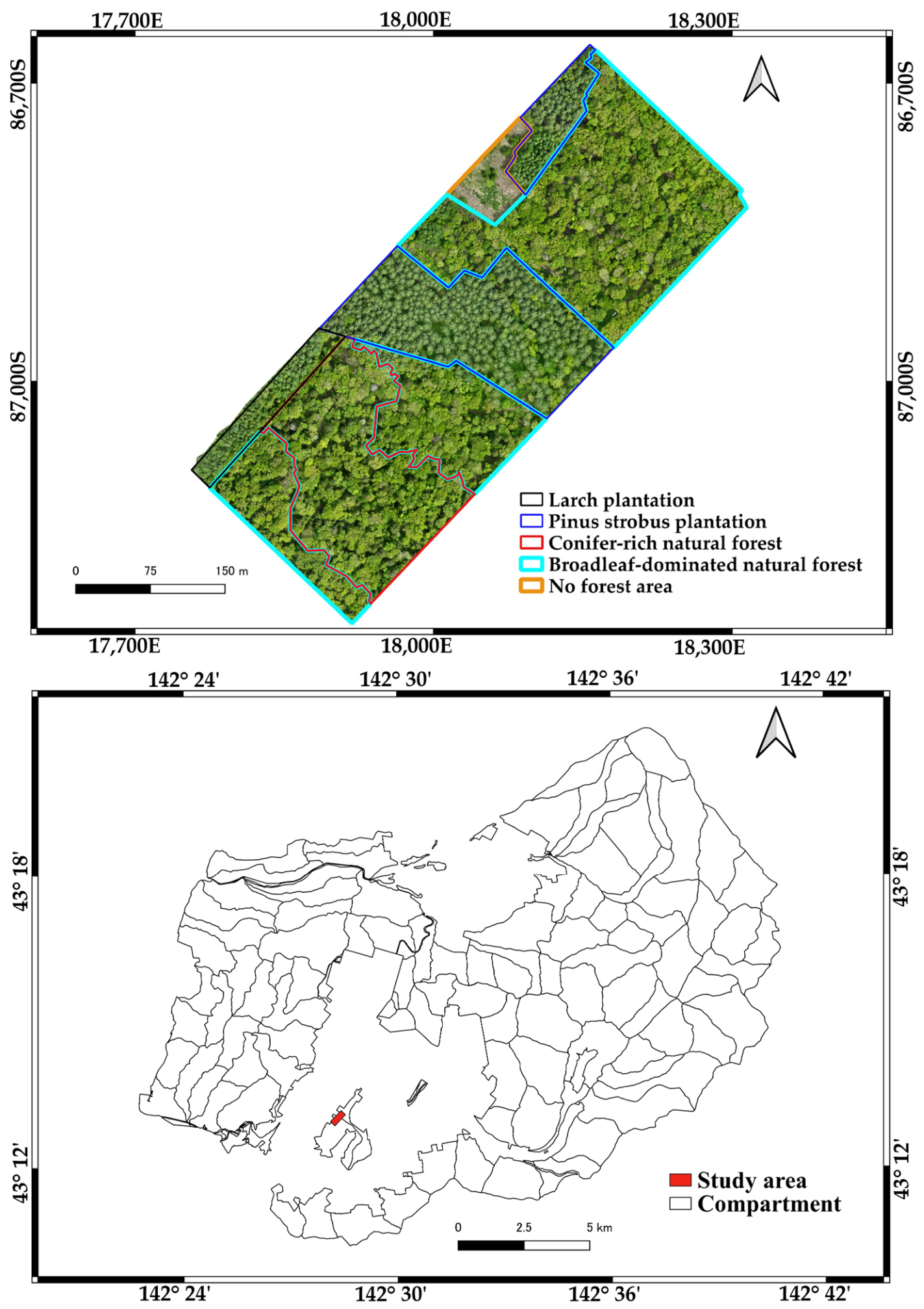
The study was conducted with an area of 14.19 ha inside the UTHF (Figure 1). Five forest categories were identified: (1) larch plantation (0.880 ha), (2) Pinus strobus plantation (3.057 ha), (3) conifer-less natural forest or broadleaf-dominated natural forest (6.655 ha), (4) conifer-rich natural forest (3.0 ha), and (5) no forest area (0.598 ha). A conifer-less natural forest was dominated by deciduous broadleaf species, including Cercidiphyllum japonicum, Ulmus davidiana var. japonica, Quercus crispula, Betula maximowicziana, Acer amoenum, Tilia japonica, and Tilia maximowicziana. A conifer-rich natural forest was composed of mixed evergreen conifers and deciduous broadleaf species, including Abies sachalinensis, Picea jezoensis, and Taxus cuspidate. In this study, we did not consider no forest area, which mainly consisted of invasive dwarf bamboo.

2.2. UAV Image Collection and Processing

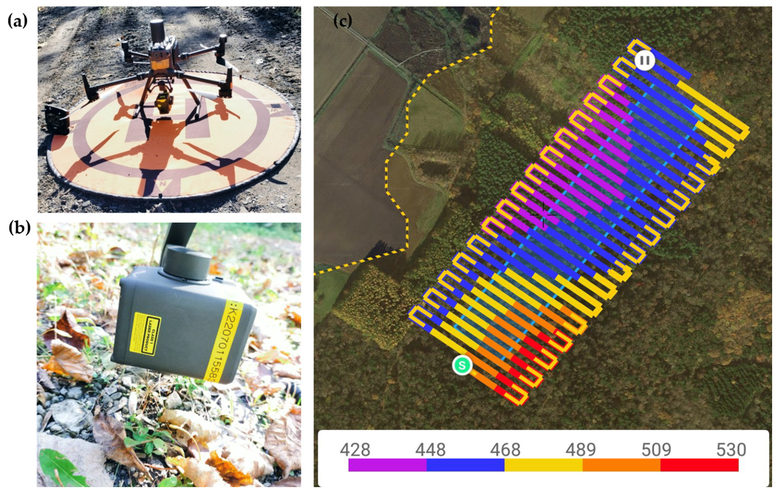
UAV survey was conducted on 24 May 2024 using a DJI Matrice 300 RTK platform equipped with the Zenmuse L2 LiDAR payload (Figure 2a,b) (SZ DJI Technology Co., Ltd., Shenzhen, China). The integrated sensor combines a LiDAR scanner, an RTK-enabled GNSS receiver, an inertial measurement unit (IMU), and a 4/3 CMOS RGB camera, enabling high-accuracy direct georeferencing and the acquisition of dense three-dimensional point clouds suitable for detailed terrain and forest characterization [40,41]. The RTK positioning system provides centimeter-level positional accuracy, eliminating the need for ground control points (GCPs) during data acquisition [42,43]. Under RTK operation, the system achieved horizontal and vertical accuracies of 1 cm and 1.5 cm, respectively [40,41]. Flight planning was performed using a grid-based mission to achieve uniform spatial coverage of the study area (Figure 2c). The survey was conducted at an altitude of 80 m above ground level with 80% forward and 80% side overlap. The flight speed was maintained at 6.3 m s⁻¹, with a ground sampling distance (GSD) of 2.18 cm pixel⁻¹, a course angle of 124°, and an average LiDAR point density of approximately 914 points m⁻².

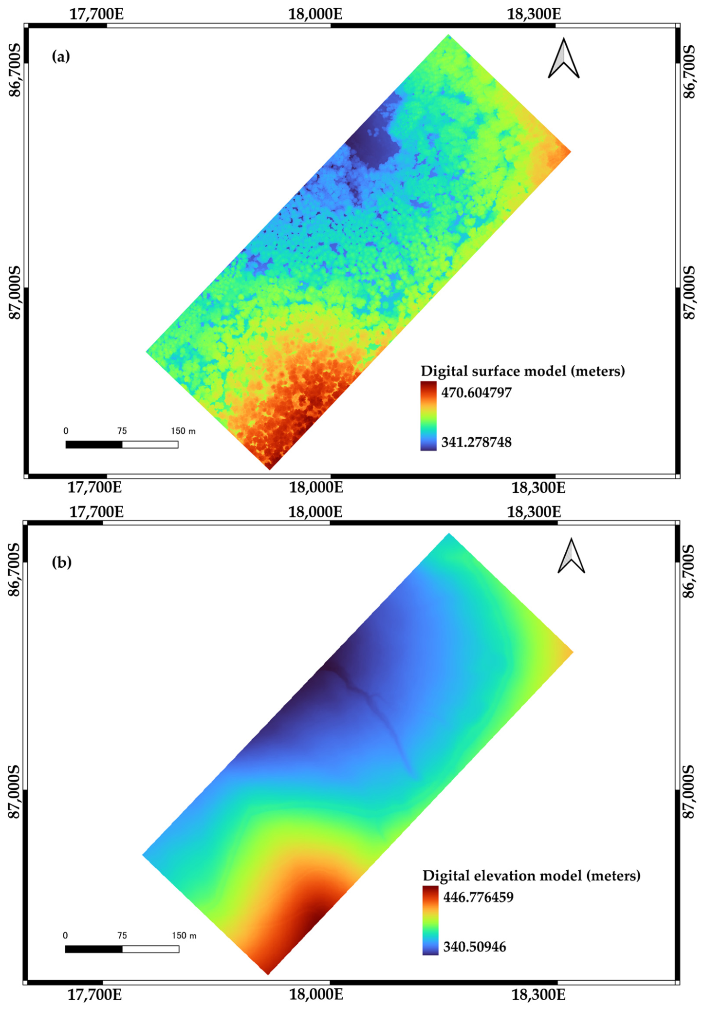
Following the survey, all datasets were transferred to a field workstation for processing in DJI Terra (Version 5.2.0), developed by DJI Enterprise. A total of 919 RGB images (focal length: 12.290 mm; sensor size: 17.923 × 13.429 mm) were processed together with the LiDAR data. The workflow consisted of four main stages: (1) data pre-processing, (2) point-cloud generation, (3) DSM and DEM generation (Figure A1), and (4) orthophoto generation. Data pre-processing was performed in standalone computation mode with both accuracy optimization and smoothing options enabled. Point clouds were generated using a density spacing of 10 cm to maintain an appropriate balance between processing efficiency and spatial resolution. Ground classification was conducted using the gentle slope algorithm with a maximum building diagonal of 20 m, an iteration angle of 6°, and an iteration distance of 0.5 m. These parameters improved the separation of ground and non-ground returns in the forested landscape, thereby enhancing terrain representation beneath vegetation. Finally, DSM, DEM, and orthophoto were generated at a spatial resolution of 50 cm.

2.3. Individual Treetop Detection

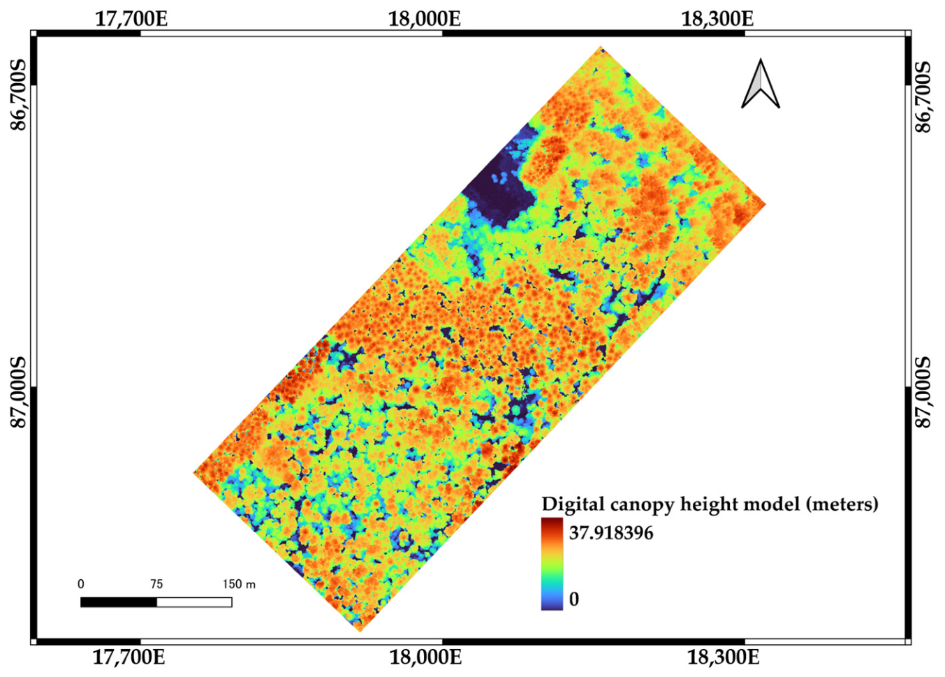
First, DCHM was derived by subtracting the DEM from the DSM [44] (Figure A2). A LM approach was employed to identify potential treetops from the generated DCHM [27]. The LM algorithm detects pixels whose height values are greater than those of the surrounding pixels within a specified moving window, assuming that each local maximum corresponds to the top of an individual tree crown [29,45,46]. To reduce false detections associated with low vegetation, shrubs, and other non-tree objects, a minimum H threshold of 2 m was applied to the DCHM prior to treetop extraction. This threshold was selected based on the field observations conducted during UAV data acquisition and visual interpretation of the orthophoto. Pixels with DCHM values below this threshold were excluded from further analysis, whereas pixels exceeding 2 m were retained as candidate canopy pixels.

Several neighborhood window sizes (3 × 3 to 29 × 29 pixels) were systematically evaluated. Smaller windows generally increase the number of detected local peaks but tend to produce multiple detections within a single crown, whereas larger windows reduce over-estimation but may fail to identify neighboring trees with overlapping canopies. Therefore, an empirical assessment was conducted by visually comparing the treetop locations generated from each window size with the corresponding high-resolution orthophoto and DCHM. Then, the reliable window size was selected, and the final LM raster was subsequently converted into a point feature dataset using the Raster Pixels to Points tool in the QGIS processing toolbox. Individual treetop detection procedure was conducted in QGIS (version 3.44.10).

2.4. Topographic Variables

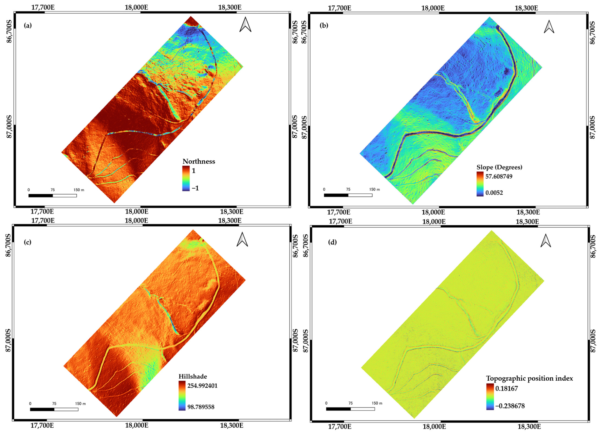
Topographic variables were derived from the DEM and generated in QGIS (version 3.44.10) using the built-in terrain analysis tools. Five topographic variables were produced: elevation, northness, slope, hillshade, and topographic position index (TPI) (Figure A3). Elevation represents the height of each location above the reference surface and was expressed in meters (m). Slope represents the local rate of change in elevation and was calculated in degrees (°). Hillshade represents the illumination intensity of the terrain based on the elevation, slope, and aspect of each location and was used as a proxy for local topographic illumination conditions. Aspect was initially derived from the DEM as the horizontal direction of slope, expressed in degrees from 0° to 360°. Aspect is a circular variable, directly treating it as an ordinary continuous predictor can introduce an artificial discontinuity between 0° and 360°. To avoid this issue, aspect was transformed into a northness index. Northness was calculated as follows.

$$\mathrm{Northness}=\cos \left(\mathrm{Aspect} \times {\displaystyle \frac{\mathsf{\pi }}{180}}\right)$$

TPI was calculated as the difference between the elevation of a focal cell and the mean elevation of its surrounding neighborhood. The resulting topographic layers were subsequently used as terrain-related predictor variables influencing H variations.

2.5. Statistical Analyses

Descriptive information on H across different forest types was stated using violin-box plot. Differences in H among forest types were assessed using the Kruskal–Wallis test. Pairwise comparisons were subsequently performed using Dunn’s post hoc test. Thereafter, GAM was applied for assessing the influence of topographic variables on H. In addition, multicollinearity among topographic (predictor) variables was assessed using the variance inflation factor (VIF), where VIF values less than 5 were considered indicative of an acceptable level of multicollinearity.

RF model was further employed to identify the relative importance of predictor variables associated with response variable [47,48]. H was specified as the response variable, whereas all remaining topographic variables were used as predictor variables. The model was implemented with 500 decision trees (ntree = 500), and the number of predictor variables randomly sampled as candidates at each split (mtry) was set to the default value for regression in the randomForest package, i.e., one-third of the total number of predictor variables. A random seed of 123 was set to ensure the reproducibility of the analysis. Variable importance was evaluated using the permutation-based importance measure [49], expressed as the percentage increase in mean squared error (% Increase in MSE). This metric quantifies the increase in prediction error after randomly permuting the values of each predictor variable. Predictor variables producing larger increases in MSE were considered more influential in predicting H. All statistical analyses were performed in R (version 4.6.0) using the FSA, car, mgcv, and randomForest packages [50,51,52,53].

3. Results

3.1. Individual Treetop Detection and Distribution Across Forest Types

Individual tree detection was performed using the local maxima method applied to the UAV-LiDAR-derived DCHM. To determine an appropriate window size for treetop detection, Multiple moving window sizes ranging from 3 × 3 to 29 × 29 pixels were evaluated to determine an appropriate window size for treetop detection. The number of detected individual trees varied substantially with window size (

Table 1. Number of detected individual trees using different local maxima window sizes.

Window Sizes (Pixels)	Number of Trees	Window Sizes (Pixels)	Number of Trees
3 × 3	234,318	17 × 17	53,753
5 × 5	166,003	19 × 19	46,803
7 × 7	129,754	21 × 21	41,012
9 × 9	104,593	23 × 23	35,864
11 × 11	86,218	25 × 25	31,349
13 × 13	72,504	27 × 27	24,468
15 × 15	62,087	29 × 29	20,641

). The number of detected trees decreased with increasing window size, from 234,318 trees using the 3 × 3 window size to 20,641 trees using the 29 × 29 window size.

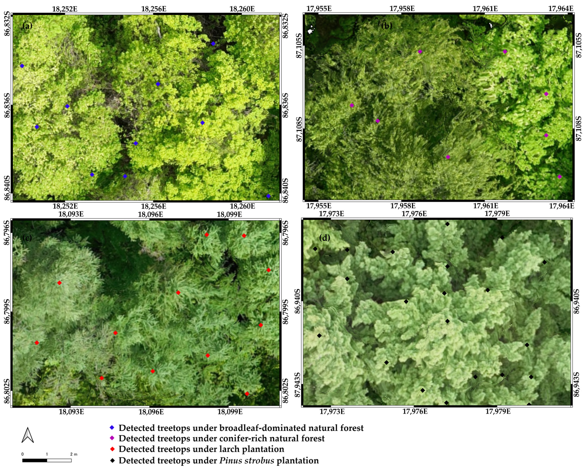
Following individual treetop detection, the optimal window sizes for each forest type were evaluated through visual interpretation of the detected treetops overlaid on the orthophoto (Figure 3). The visual assessment revealed that the optimal window size varied among four forest types. For the broadleaf-dominated natural forest, a 27 × 27 window size provided the most appropriate representation of individual treetops (Figure 3a). In the conifer-rich natural forest, the 29 × 29 window size was identified as the optimal window size (Figure 3b). For the larch plantation, a 25 × 25 window size produced the most appropriate treetop detection (Figure 3c), whereas a 21 × 21 window size was considered most suitable for the Pinus strobus plantation (Figure 3d).

The optimal window size differed among forest types, with larger window sizes being selected for the natural forests (27 × 27 and 29 × 29 pixels) compared with the plantations (25 × 25 and 21 × 21 pixels) (Figure 3). A total of 26,886 trees were detected among four forest types. The broadleaf-dominated natural forest had the largest total number of detected trees, with 11,555 trees identified across an area of 6.655 ha, corresponding to an estimated tree density of 1736 trees ha⁻¹. The conifer-rich natural forest consisted of 3721 detected trees over 3.0 ha, resulting in a lower estimated tree density of 1240 trees ha⁻¹. Among the plantation forests, 1027 individual trees were detected within the larch plantation, which covered 0.880 ha, corresponding to an estimated tree density of 1167 trees ha⁻¹. In contrast, the Pinus strobus plantation had the highest tree density among all four forest types, with 10,583 detected trees across 3.057 ha (

Table 2. Detected tree numbers across four forest types.

	Detected Number of Trees in Total	Areas in Total (ha)	Estimated Tree Density (Trees/ha)	Selected Window-Size
Broadleaf-dominated natural forest	11,555	6.655	1736	27 × 27
Conifer-rich natural forest	3721	3.000	1240	29 × 29
Larch plantation	1027	0.880	1167	25 × 25
Pinus strobus plantation	10,583	3.057	3462	21 × 21

).

3.2. Canopy Height Across Forest Types

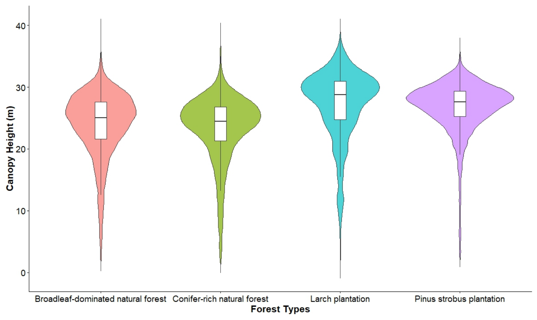
The distribution of H varied among the forest types (Figure 4). The larch plantation exhibited the highest maximum H (37.918 m), followed by Pinus strobus plantation (35.648 m), broadleaf-dominated natural forest (34.194 m), and conifer-rich natural forest (32.238 m). The minimum H had 2.066 m in the broadleaf-dominated natural forest. Figure 4 further indicated that the median H was highest in the larch plantation, whereas the conifer-rich natural forest showed the lowest median H. In addition, differences in the distribution and variability of H are revealed among forest types, with the larch plantation and Pinus strobus plantation exhibiting relatively higher concentrations of H between approximately 25 and 30 m (Figure 4).

Additionally, the Kruskal–Wallis test confirmed that H differed significantly among four forest types (χ² = 3078.809, p < 0.001;

Table 3. Result of the Kruskal–Wallis test examining differences in H among forest types.

Response Variable	χ2	p-Value
Canopy height	3078.809	<2.2 × 10−16

).

Pairwise comparisons also indicated significant differences in H between forest types (

Table 4. Pairwise comparisons of H among forest types using Dunn’s post hoc test.

H Comparison	Z-Value	Adjusted p-Value
Broadleaf-dominated natural forest vs. Conifer-rich natural forest	7.880	<0.001
Broadleaf-dominated natural forest vs. Larch plantation	−23.519	<0.001
Broadleaf-dominated natural forest vs. Pinus strobus plantation	−46.497	<0.001
Conifer-rich natural forest vs. Larch plantation	−25.939	<0.001
Conifer-rich natural forest vs. Pinus strobus plantation	−40.618	<0.001
Larch plantation vs. Pinus strobus plantation	4.289	0.173

Note: p-values were adjusted using the Bonferroni correction.

). Specifically, significant differences were observed between broadleaf-dominated natural forest and conifer-rich natural forest, broadleaf-dominated natural forest and larch plantation, broadleaf-dominated natural forest and Pinus strobus plantation, conifer-rich natural forest and larch plantation, and conifer-rich natural forest and Pinus strobus plantation (adjusted p < 0.001). In contrast, H did not differ significantly between larch plantation and Pinus strobus plantation (adjusted p = 0.173) (Table 4).

3.3. Canopy Height Variations Across Topography

The analysis revealed that the relationships between H and topographic variables differed among forest types (

Table 5. GAM-based assessment of topographic drivers affecting forest canopy heights.

	edf	Ref.df	F	p-Value
Broadleaf-dominated natural forest (Adjusted R2 = 0.142)
Elevation	8.827	8.991	122.997	<2 × 10−16 ***
Slope	6.492	7.680	10.020	<2 × 10−16 ***
Northness	7.694	8.573	23.830	<2 × 10−16 ***
Hillshade	7.603	8.523	7.195	<2 × 10−16 ***
Topographic position index	2.173	2.870	1.160	0.346
Conifer-rich natural forest (Adjusted R2 = 0.104)
Elevation	8.308	8.869	18.255	<2 × 10−16 ***
Slope	4.892	6.057	5.727	6.8 × 10−6 ***
Northness	3.355	4.286	1.810	0.142
Hillshade	6.087	7.279	8.612	<2 × 10−16 ***
Topographic position index	1.089	1.173	0.739	0.362
Larch plantation (Adjusted R2 = 0.125)
Elevation	6.084	7.254	8.477	<2 × 10−16 ***
Slope	3.694	4.688	6.123	3.2 × 10−5 ***
Northness	3.651	4.607	2.841	0.018 *
Hillshade	3.176	4.042	4.265	0.002 *
Topographic position index	2.275	2.977	1.139	0.359
Pinus strobus plantation (Adjusted R2 = 0.071)
Elevation	8.580	8.949	52.039	<2 × 10−16 ***
Slope	4.336	5.428	6.833	2.1 × 10−6 ***
Northness	6.361	7.507	11.915	<2 × 10−16 ***
Hillshade	5.141	6.384	34.335	<2 × 10−16 ***
Topographic position index	4.592	5.777	2.125	0.038 *

Note: *** Significant at p < 0.001, * Significant at p < 0.05.

). In the broadleaf-dominated natural forest, elevation, slope, Northness, and hillshade were all associated with H (p < 0.001), whereas TPI was not significant (p = 0.346). The relatively high effective degrees of freedom (edf = 6.492–8.827) indicate that these relationships were predominantly nonlinear. The GAM explained 14.2% of the variation in H, with an adjusted R² of 0.142.

In the conifer-rich natural forest, H exhibited a significant relationship with elevation, slope, and hillshade (p = 0.001). In contrast, Northness (p = 0.142) and TPI (p = 0.362) were not associated with H. The edf values ranging from 4.892 to 8.308 suggest the nonlinear relationships between H and topographic variables. The model had an adjusted R² value of 0.104.

For the larch plantation, elevation and slope influence H (p < 0.001). In addition, northness and hillshade also showed relationships with H (p = 0.018 and 0.002). However, TPI was not related to H (p > 0.05). The model explained 12.5% of the variation in H (adjusted R² = 0.125).

In the Pinus strobus plantation, all topographic variables showed relationships with H. Elevation, slope, northness, and hillshade had effects on canopy H at p < 0.001. Despite the statistical relationships, the model had the lowest explanatory power among the four forest types, with an adjusted R² of 0.071 (Table 5).

Overall, the GAM results indicate that the topographic variables affecting H differed among forest types. Elevation, slope, and hillshade were consistently significant across all four forest types. Northness was significant in the broadleaf-dominated natural forest, larch plantation, and Pinus strobus plantation, but not in the conifer-rich natural forest. TPI was generally not significant, except in the Pinus strobus plantation.

Multicollinearity among predictor variables was separately assessed for each forest type using VIF (

Table 6. Variance inflation factor values of the predictor variables used in the model.

	Elevation	Slope	Northness	Hillshade	TPI
For broadleaf-dominated natural forest	1.482	1.532	1.065	1.066	1.016
For conifer-rich natural forest	1.229	1.266	1.528	1.331	1.019
For larch plantation	2.052	2.247	1.805	1.615	1.003
For Pinus strobus plantation	1.278	1.215	1.086	1.113	1.007

). Across all forest types, VIF values ranged from 1.003 to 2.247 (Table 6). All VIF values were below the accepted threshold of 5, indicating that multicollinearity was not a concern in the model.

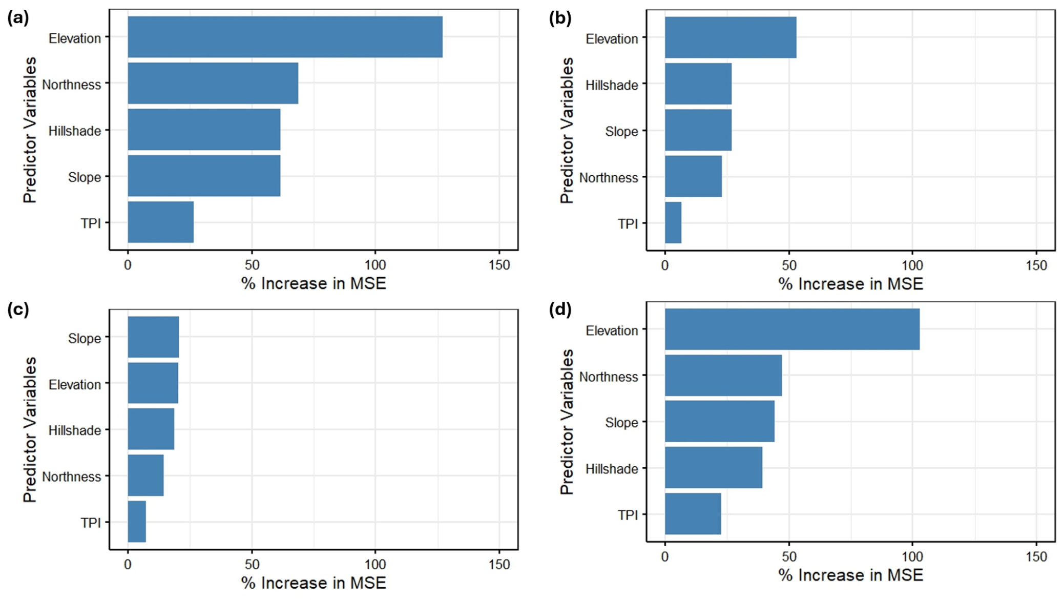
Furthermore, RF model revealed differences in the relative importance of topographic variables among forest types (Figure 5). In the broadleaf-dominated natural forest, elevation was identified as the most influential predictor of H (% Increase in MSE = 127.240), followed by northness (68.671), hillshade (61.615), slope (61.451), and TPI (26.554). Similarly, elevation was the most important predictor of H in the conifer-rich natural forest (% Increase in MSE = 53.176), followed by hillshade (27.007), slope (26.813), northness (23.057), and TPI (6.505).

In the larch plantation, slope exhibited the highest importance (% Increase in MSE = 20.801), followed by elevation (20.446), hillshade (18.706), northness (14.487), and TPI (7.205). In contrast, elevation remained the dominant predictor in the Pinus strobus plantation (% Increase in MSE = 103.013), followed by northness (47.102), slope (44.185), hillshade (39.321), and TPI (22.505). Overall, elevation was the most influential topographic variable in three of four forest types. In contrast, TPI consistently exhibited the lowest variable importance across all forest types, indicating a relatively limited contribution to explaining H variation (Figure 5).

4. Discussion

4.1. Individual Treetop Detection and Distribution

The UAV-LiDAR-derived DCHM combined with the local maxima algorithm provided an effective way for detecting individual trees and quantifying H variations across different forest types and topography. The number of detected trees decreased with increasing moving window size, reflecting the sensitivity of the local maxima algorithm to window size selection (Table 1). The optimal window size was 27 × 27 pixels for the broadleaf-dominated natural forest, 29 × 29 pixels for the conifer-rich natural forest, 25 × 25 pixels for the larch plantation, and 21 × 21 pixels for the Pinus strobus plantation (Figure 3). This variation indicates that a single fixed window size may not adequately represent the structural characteristics of different forest stands. Similar observations have been reported in previous studies [27,54,55], where optimal window sizes substantially improved individual tree detection accuracy by balancing over- and under-estimation of tree numbers. In particular, smaller windows tend to increase the number of detected treetops but can also increase false detections, whereas larger windows generally reduce commission errors at the expense of missing smaller or closely spaced trees.

The relatively large optimal window sizes observed in the two natural forests may be associated with their more heterogeneous canopy structures and greater spatial overlap among crowns. In natural forests, trees commonly differ in species, age, crown dimensions, height, and spatial arrangement, resulting in irregular canopy surfaces with multiple treetops. A local maxima algorithm identifies a treetop based primarily on the highest elevation within a defined neighborhood; therefore, the selection of an appropriate neighborhood size becomes particularly important where adjacent crowns overlap or where multiple small treetops occur within a single crown. Broadleaf trees can present an additional challenge because their crowns are often irregular and may contain several local high points rather than a single clearly defined treetop. Consequently, a relatively large moving window size may have been necessary in the natural forests to reduce the identification of multiple treetops within individual crowns. The plantation forests, in contrast, required somewhat smaller window sizes, particularly the Pinus strobus plantation. The homogeneous species composition and regular stand structure of plantations may produce more consistently shaped crowns and more clearly separated canopy tops. Under these conditions, a smaller window can distinguish neighboring treetops more effectively without generating an excessive number of false treetops.

The differences in detected tree density among the different forest types should also be cautiously interpreted in this study because the number of detected trees is influenced by the characteristics of the detection algorithm and the visual interpretation of orthophoto. The broadleaf-dominated natural forest contained an estimated tree density of 1736 trees ha⁻¹, whereas the conifer-rich natural forest had 1240 trees ha⁻¹. The larch plantation had the lowest detected tree density among the four forest types, at 1167 trees ha⁻¹, while the Pinus strobus plantation had the highest detected tree density, at approximately 3462 trees ha⁻¹ (Table 2). The particularly high detected tree density in the Pinus strobus plantation may reflect a combination of high actual tree density and the relatively small optimal detection window, which allowed the more closely spaced canopy tops to be distinguished. Therefore, in the present study, the detected tree densities can be regarded primarily as algorithm-derived structural indicators unless they are independently validated against field-based tree inventories.

The present study differs from previous study in several important respects. First, whereas Rahman [18] used airborne LiDAR over a large regional area, the present study uses a UAV-LiDAR system to acquire very high-density point-cloud data within a relatively small forest landscape, allowing canopy structure to be examined at a high spatial resolution. Second, the present study explicitly focuses on individual-tree height derived from a high-resolution 50 cm DCHM, and the LM window size is empirically evaluated across multiple window sizes before individual treetops are extracted. This approach is intended to better accommodate differences in crown size and stand structure among forest types rather than applying a single fixed detection scale. Third, the present study distinguishes two plantation types (larch and Pinus strobus) and two natural forests (coni-fer-rich and broadleaf-dominated natural forests), thereby allowing canopy height differences to be examined in relation to more specific local forest structural conditions. Fourth, rather than incorporating neighborhood tree density, canopy-gap distance, and stand age as explanatory variables, the present study focuses specifically on local topographic controls represented by elevation, northness, slope, hillshade, and TPI. Finally, GAM and RF analyses were used to examine potentially nonlinear relationships and the relative importance of topographic variables.

4.2. Differences in Canopy Height Among Forest Types

Significant differences in H were observed among forest types (Table 3 and Table 4), indicating substantial variation in forest structural characteristics. The higher H observed in the plantations, particularly the larch plantation (Figure 4), may be related to differences in stand development, species composition, and management history. Although the larch plantation exhibited the highest H, no significant difference was observed between the larch plantation and Pinus strobus plantation (Table 4). In contrast, both plantation forests differed significantly from the natural forests, reflecting differences in species composition, stand development, and structural complexity. Planted forests have more uniform species composition and stand structure than natural forests, and management practices may influence stand density, age structure, and competitive interactions. These factors can result in relatively homogeneous canopy development and the formation of tall dominant trees. Natural forests generally consist of multiple tree species, variable crown architectures, and uneven-aged stands, whereas plantation forests are typically characterized by more uniform canopy structures resulting from silvicultural management. The significant differences in H among forest types indicate that comparisons of H across heterogeneous forest landscapes should account for forest composition and stand type. This is particularly relevant for applications involving biomass estimation, forest growth assessment, habitat characterization, or forest structural monitoring, because differences in H may reflect both biological differences among forest types and differences in stand development or management history.

4.3. Influence of Topographic Factors on Canopy Height

The GAM analysis demonstrated that H was influenced by topographic variables (Table 5), suggesting that forest type responds to the influence of topographic conditions on canopy development. However, the strength and composition of these relationships varied among forest types. Elevation, slope, and hillshade were the influential predictors in all four forest types, whereas Northness was significant in three forest types and TPI was significant only in the Pinus strobus plantation. These findings indicate that topographic influence on H is not uniform across forest types. Instead, the relationship between canopy structure and terrain appears to depend partly on the structural characteristics of individual stands.

Elevation exhibited relationships with H in all forest types (Table 5), suggesting that elevation captures important spatial gradients in growing conditions of the trees [56]. The importance of elevation was particularly evident in the RF analysis. Elevation was the most important predictor in the broadleaf-dominated natural forest, conifer-rich natural forest, and Pinus strobus plantation, whereas slope ranked first in the larch plantation (Figure 5). The consistency between the GAM and RF analyses strengthens the findings that elevation represents an important factor affecting canopy height. However, elevation may be correlated with several environmental factors, including temperature, moisture availability, exposure, and soil development. The present analysis did not directly include these ecological variables, the observed statistical relationship should not be interpreted as evidence that elevation itself directly controls H. Rather, elevation may act as a proxy for a combination of environmental gradients that influence tree growth and canopy development.

The effects of other topographic variables also differed among forest types. Slope exhibited the relationships with H across all forest types. Steeper terrain can be related to differences in soil depth and water availability, which may affect tree growth. In addition, steep slopes can influence the spatial distribution of trees and competition for resources. Therefore, the observed relationship between slope and H may reflect the conditions of ecological and geometric effects. Hillshade was another influential predictor across all forest types. Hillshade represents relative terrain illumination rather than direct solar radiation, its influence is likely associated with differences in light availability and moisture conditions [57]. Its significance suggests that spatial differences in terrain illumination may correspond to canopy development. Therefore, its relationship with H should be interpreted as a topographic proxy rather than direct evidence of a light-driven growth response.

Northness showed a more forest-type-specific pattern. It affects H of broadleaf-dominated natural forest, larch plantation, and Pinus strobus plantation, but not in the conifer-rich natural forest. This difference suggests that aspect-related environmental gradients may interact with forest composition and stand structure. Differences in species-specific light requirements could potentially contribute to the contrasting response among forest types. TPI showed the weakest relationship with canopy height (Table 5). The consistently low RF importance of TPI further supports its relatively limited contribution to explaining H variation in the present dataset (Figure 5). This result may indicate that local relative topographic position was less important than elevation, slope, or illumination-related gradients at the spatial scale.

4.4. Complementary Interpretations of Generalized Additive Model and Random Forest Model Results

The analysis of GAM and RF provided complementary information about the relationship between H and topographic variables. The relatively high effective degrees of freedom under GAM analysis indicate that the relationships between canopy height and topographic variables were not represented by simple linear relationships. GAM identified statistically nonlinear relationships, whereas RF provided a ranking of the relative predictive importance of the topographic variables. The application of these two approaches provides stronger evidence that certain topographic variables are consistently relevant to H variation. For example, elevation was the most important RF predictor in the broadleaf-dominated natural forest, conifer-rich natural forest, and Pinus strobus plantation. This result corresponds with its statistical significance in the GAM analyses for all four forest types. The agreement between the two modeling approaches suggests that elevation contains substantial information related to spatial variation in H. In the larch plantation, however, slope ranked slightly higher than elevation in RF importance, despite both variables being significant in the GAM analysis. The relatively low RF importance of TPI across all forest types provides an additional indication that local relative topographic position contributed less to predicting H than other topographic factors. Nevertheless, the predictor importance ranking should be interpreted together with the GAM results rather than independently. The GAM results provide evidence regarding statistical relationships, while RF captures potentially complex interactions and nonlinear predictive contributions. Using both approaches is consequently useful for identifying robust patterns while avoiding overreliance on a single modeling framework.

4.5. Implications for UAV-LiDAR-Based Forest Structural Assessment

The present study demonstrates an effective application of UAV-LiDAR for assessing differences in forest structure among forest types and across heterogeneous terrain. The ability to identify individual treetops and quantify canopy height at high spatial resolution provides information that is difficult to obtain consistently through conventional field measurements alone. The forest-type-specific optimal window sizes further demonstrate that UAV-LiDAR-based individual treetop detection with local maxima algorithm can be adapted to different canopy structures rather than relying on a universal parameterization. The findings also demonstrate that H should be considered as an indicator of both forest structure and environmental heterogeneity. The significant differences in H among forest types demonstrate the importance of stand composition and management history. From a forest management perspective, UAV-LiDAR can provide detailed information on H that may support forest inventory, stand structural assessment, and identification of spatially heterogeneous areas.

4.6. Research Limitations

The present study has research limitations. First, the optimal local maxima window sizes were selected through visual interpretation of treetops overlaid on orthophotos. This approach provides a practical basis for the extraction of canopy height values of detected trees. However, in this study, the canopy height values of detected trees were not validated using field-measured tree heights. Consequently, omission and commission errors associated with canopy height values could not be quantitatively evaluated.

Second, the present study considered the influence of topographic factors, including elevation, slope, northness, hillshade, and TPI, but H is influenced by numerous biological and environmental factors that were not considered in this study. The relatively low adjusted R² values indicate that these omitted variables are likely important sources of variation. Although the VIF results indicated low multicollinearity among the predictor variables, low multicollinearity does not imply that the models capture the principal factors affecting tree height. The VIF values of 1.003–2.247 indicate that the predictors were not strongly redundant, but the low model explanatory power demonstrates that additional explanatory variables are still required. Future research could therefore consider the influence of management history, stand age, site index, crown dimensions, soil properties, disturbance history, canopy-gap characteristics, and microclimatic variables.

5. Conclusions

This study confirms that UAV-LiDAR effectively captures forest type- and topography-driven variations in H. The local maxima method successfully detected individual trees from the UAV-LiDAR-derived DCHM, and the optimal window sizes for different forest types provided a reliable estimate of tree densities that were consistent with visual interpretation of the orthophoto. The results revealed significant H variations among forest types, although no significant difference was detected between the larch plantation and Pinus strobus plantation. Furthermore, the relationships between H and topographic variables varied among forest types. Generalized additive model indicated that elevation exhibited the relationship with H in all forest types. In contrast, TPI showed no significant relationship with H in any forest type, except Pinus strobus plantation. RF model further demonstrated that elevation was the most influential topographic predictor in the broadleaf-dominated natural forest, conifer-rich natural forest, and Pinus strobus plantation, whereas slope was the dominant predictor in the larch plantation. Overall, TPI consistently exhibited the lowest importance for explaining H variation across all forest types.

These findings indicate that the influence of topography on forest H is dependent on forest type and highlight the importance of considering forest type when evaluating topographic controls on forest structure. Overall, the findings contribute to a better understanding of the influence of forest types and topographic conditions on forest canopy structure and provide valuable information for forest inventory. Further studies should investigate the influence of additional environmental factors, such as soil properties, stand age, and climatic conditions, on H variations. In addition, future research integrating the individual treetop detection method with field data validation may provide additional insights to improve the accuracy of H estimation.

References

1. Kay, H.; Santoro, M.; Cartus, O.; Bunting, P.; Lucas, R. Exploring the Relationship between Forest Canopy Height and Canopy Density from Spaceborne Lidar Observations. Remote Sens. 2021, 13, 4961. [Google Scholar] [CrossRef] [Scilit]
2. Marselis, S.M.; Tang, H.; Armston, J.; Abernethy, K.; Alonso, A.; Barbier, N.; Bissiengou, P.; Jeffery, K.; Kenfack, D.; Labrière, N.; et al. Exploring the Relation between Remotely Sensed Vertical Canopy Structure and Tree Species Diversity in Gabon. Environ. Res. Lett. 2019, 14, 94013. [Google Scholar] [CrossRef] [Scilit]
3. Win, K.; Thein, T.T.; Tun, P.P.; Chan, N.; Hiroshima, T.; Sato, T. Remote Sensing and Deep Learning-Based Detection of Changes in Aboveground Carbon Storage in Young Teak Plantations (2019–2023): A Case Study in Pauk Khaung Township, West Bago Mountains, Myanmar. Geomatica 2025, 77, 100074. [Google Scholar] [CrossRef] [Scilit]
4. Alaniz, A.J.; Carvajal, M.A.; Fierro, A.; Vergara-Rodríguez, V.; Toledo, G.; Ansaldo, D.; Moreira-Arce, D.; Rojas-Osorio, A.; Vergara, P.M. Remote-Sensing Estimates of Forest Structure and Dynamics as Indicators of Habitat Quality for Magellanic Woodpeckers. Ecol. Indic. 2021, 126, 107634. [Google Scholar] [CrossRef] [Scilit]
5. Moles, A.T.; Warton, D.I.; Warman, L.; Swenson, N.G.; Laffan, S.W.; Zanne, A.E.; Pitman, A.; Hemmings, F.A.; Leishman, M.R. Global Patterns in Plant Height. J. Ecol. 2009, 97, 923–932. [Google Scholar] [CrossRef] [Scilit]
6. Xu, Y.; Li, C.; Sun, Z.; Jiang, L.; Fang, J. Tree Height Explains Stand Volume of Closed-Canopy Stands: Evidence from Forest Inventory Data of China. For. Ecol. Manag. 2019, 438, 51–56. [Google Scholar] [CrossRef] [Scilit]
7. Zhang, J.; Nielsen, S.E.; Mao, L.; Chen, S.; Svenning, J.C. Regional and Historical Factors Supplement Current Climate in Shaping Global Forest Canopy Height. J. Ecol. 2016, 104, 469–478. [Google Scholar] [CrossRef] [Scilit]
8. Pan, X.; Ji, J.; Gao, K.; Wei, T.; He, M.; Zhang, X. Divergent Responses of Forest Canopy Height to Environmental Conditions across China. Ecol. Indic. 2024, 168, 112763. [Google Scholar] [CrossRef] [Scilit]
9. Laginha Pinto Correia, D.; Raulier, F.; Filotas, É.; Bouchard, M. Stand Height and Cover Type Complement Forest Age Structure as a Biodiversity Indicator in Boreal and Northern Temperate Forest Management. Ecol. Indic. 2017, 72, 288–296. [Google Scholar] [CrossRef] [Scilit]
10. Ri, A.; An, H. Health Assessment of Natural Larch Forest in Arxan Guided by Forestry Remote Sensing Integrated with Canopy Feature Analysis. Front. Environ. Sci. 2023, 11, 1171660. [Google Scholar] [CrossRef] [Scilit]
11. Gorgens, E.B.; Nunes, M.H.; Jackson, T.; Coomes, D.; Keller, M.; Reis, C.R.; Valbuena, R.; Rosette, J.; de Almeida, D.R.A.; Gimenez, B.; et al. Resource Availability and Disturbance Shape Maximum Tree Height across the Amazon. Glob. Change Biol. 2021, 27, 177–189. [Google Scholar] [CrossRef] [Scilit] [PubMed]
12. Sexton, J.O.; Bax, T.; Siqueira, P.; Swenson, J.J.; Hensley, S. A Comparison of Lidar, Radar, and Field Measurements of Canopy Height in Pine and Hardwood Forests of Southeastern North America. For. Ecol. Manag. 2009, 257, 1136–1147. [Google Scholar] [CrossRef] [Scilit]
13. Martin, A.J.F. Accuracy and Precision in Urban Forestry Tools for Estimating Total Tree Height. Arboric. Urban For. 2022, 48, 319–332. [Google Scholar] [CrossRef] [Scilit]
14. De Petris, S.; Sarvia, F.; Borgogno-mondino, E. About Tree Height Measurement: Theoretical and Practical Issues for Uncertainty Quantification and Mapping. Forests 2022, 13, 969. [Google Scholar] [CrossRef] [Scilit]
15. Win, K.; Sato, T. Influence of Stand Characteristics and Management Activities on Aboveground Carbon Storage in Japanese Cedar and Cypress Plantations: Sustainable Management Implications. Trees For. People 2024, 18, 100702. [Google Scholar] [CrossRef] [Scilit]
16. Wang, Y.; Lehtomäki, M.; Liang, X.; Pyörälä, J.; Kukko, A.; Jaakkola, A.; Liu, J.; Feng, Z.; Chen, R.; Hyyppä, J. Is Field-Measured Tree Height as Reliable as Believed—A Comparison Study of Tree Height Estimates from Field Measurement, Airborne Laser Scanning and Terrestrial Laser Scanning in a Boreal Forest. ISPRS J. Photogramm. Remote Sens. 2019, 147, 132–145. [Google Scholar] [CrossRef] [Scilit]
17. Wang, Q.; Ni-Meister, W. Forest Canopy Height and Gaps from Multiangular BRDF, Assessed with Airborne LiDAR Data (Short Title: Vegetation Structure from LiDAR and Multiangular Data). Remote Sens. 2019, 11, 2566, Erratum in Remote Sens. 2021, 13, 17. https://doi.org/10.3390/rs13010017. [Google Scholar] [CrossRef] [Scilit]
18. Farhadur Rahman, M.; Onoda, Y.; Kitajima, K. Forest Canopy Height Variation in Relation to Topography and Forest Types in Central Japan with LiDAR. For. Ecol. Manag. 2022, 503, 119792. [Google Scholar] [CrossRef] [Scilit]
19. Popescu, S.C.; Wynne, R.H.; Nelson, R.F. Estimating Plot-Level Tree Heights with Lidar: Local Filtering with a Canopy-Height Based Variable Window Size. Comput. Electron. Agric. 2002, 37, 71–95. [Google Scholar] [CrossRef] [Scilit]
20. Takagi, K.; Yone, Y.; Takahashi, H.; Sakai, R.; Hojyo, H.; Kamiura, T.; Nomura, M.; Liang, N.; Fukazawa, T.; Miya, H.; et al. Forest Biomass and Volume Estimation Using Airborne LiDAR in a Cool-Temperate Forest of Northern Hokkaido, Japan. Ecol. Inform. 2015, 26, 54–60. [Google Scholar] [CrossRef] [Scilit]
21. Wang, D.; Wan, B.; Qiu, P.; Zuo, Z.; Wang, R.; Wu, X. Mapping Height and Aboveground Biomass of Mangrove Forests on Hainan Island Using UAV-LiDAR Sampling. Remote Sens. 2019, 11, 2156. [Google Scholar] [CrossRef] [Scilit]
22. Deng, S.; Jing, S.; Zhao, H. A Hybrid Method for Individual Tree Detection in Broadleaf Forests Based on UAV-LiDAR Data and Multistage 3D Structure Analysis. Forests 2024, 15, 1043. [Google Scholar] [CrossRef] [Scilit]
23. Picos, J.; Bastos, G.; Míguez, D.; Alonso, L.; Armesto, J. Individual Tree Detection in a Eucalyptus Plantation Using Unmanned Aerial Vehicle (UAV)-LiDAR. Remote Sens. 2020, 12, 885. [Google Scholar] [CrossRef] [Scilit]
24. You, H.; Liu, Y.; Lei, P.; Qin, Z.; You, Q. Segmentation of Individual Mangrove Trees Using UAV-Based LiDAR Data. Ecol. Inform. 2023, 77, 102200. [Google Scholar] [CrossRef] [Scilit]
25. Ma, K.; Chen, Z.; Fu, L.; Tian, W.; Jiang, F.; Yi, J.; Du, Z.; Sun, H. Performance and Sensitivity of Individual Tree Segmentation Methods for UAV-LiDAR in Multiple Forest Types. Remote Sens. 2022, 14, 298. [Google Scholar] [CrossRef] [Scilit]
26. Fu, Y.; Niu, Y.; Wang, L.; Li, W. Individual-Tree Segmentation from UAV–LiDAR Data Using a Region-Growing Segmentation and Supervoxel-Weighted Fuzzy Clustering Approach. Remote Sens. 2024, 16, 608. [Google Scholar] [CrossRef] [Scilit]
27. Hudjimartsu, S.A.; Purnomo, M.R.; Yanuarsyah, I.; Sianturi, V.; Sulistiyono, N. Optimizing Local Maxima Parameters for UAV-Based Detection of Pinus Merkusii in Tropical Forest Plantations. Eur. J. Remote Sens. 2026, 59, 2697336. [Google Scholar] [CrossRef] [Scilit]
28. Schaller, C.; Ginzler, C.; van Loon, E.; Moos, C.; Seijmonsbergen, A.C.; Dorren, L. Improving Country-Wide Individual Tree Detection Using Local Maxima Methods Based on Statistically Modeled Forest Structure Information. Int. J. Appl. Earth Obs. Geoinf. 2023, 123, 103480. [Google Scholar] [CrossRef] [Scilit]
29. Azizi, Z.; Miraki, M. Individual Urban Trees Detection Based on Point Clouds Derived from UAV-RGB Imagery and Local Maxima Algorithm, a Case Study of Fateh Garden, Iran. Environ. Dev. Sustain. 2024, 26, 2331–2344. [Google Scholar] [CrossRef] [Scilit]
30. Bałazy, R.; Kamińska, A.; Ciesielski, M.; Socha, J.; Pierzchalski, M. Modeling the Effect of Environmental and Topographic Variables Affecting the Height Increment of Norway Spruce Stands in Mountainous Conditions with the Use of LiDAR Data. Remote Sens. 2019, 11, 2407. [Google Scholar] [CrossRef] [Scilit]
31. Tsunoda, Y.; Tsuda, T.; Ohno, Y. Influence of Stand Structure on Tree Height: A Comparative Study across 46 Species. For. Ecol. Manag. 2025, 578, 122474. [Google Scholar] [CrossRef] [Scilit]
32. Jucker, T.; Bongalov, B.; Burslem, D.F.R.P.; Nilus, R.; Dalponte, M.; Lewis, S.L.; Phillips, O.L.; Qie, L.; Coomes, D.A. Topography Shapes the Structure, Composition and Function of Tropical Forest Landscapes. Ecol. Lett. 2018, 21, 989–1000. [Google Scholar] [CrossRef] [Scilit] [PubMed]
33. Ediriweera, S.; Danaher, T.; Pathirana, S. The Influence of Topographic Variation on Forest Structure in Two Woody Plant Communities: A Remote Sensing Approach. For. Syst. 2016, 25, e049. [Google Scholar] [CrossRef] [Scilit]
34. Fricker, G.A.; Synes, N.W.; Serra-Diaz, J.M.; North, M.P.; Davis, F.W.; Franklin, J. More than Climate? Predictors of Tree Canopy Height Vary with Scale in Complex Terrain, Sierra Nevada, CA (USA). For. Ecol. Manag. 2019, 434, 142–153. [Google Scholar] [CrossRef] [Scilit]
35. Muscarella, R.; Kolyaie, S.; Morton, D.C.; Zimmerman, J.K.; Uriarte, M. Effects of Topography on Tropical Forest Structure Depend on Climate Context. J. Ecol. 2020, 108, 145–159. [Google Scholar] [CrossRef] [Scilit]
36. Mielcarek, M.; Stereńczak, K.; Khosravipour, A. Testing and Evaluating Different LiDAR-Derived Canopy Height Model Generation Methods for Tree Height Estimation. Int. J. Appl. Earth Obs. Geoinf. 2018, 71, 132–143. [Google Scholar] [CrossRef] [Scilit]
37. Xu, D.; Wang, H.; Xu, W.; Luan, Z.; Xu, X. LiDAR Applications to Estimate Forest Biomass at Individual Tree Scale: Opportunities, Challenges and Future Perspectives. Forests 2021, 12, 550. [Google Scholar] [CrossRef] [Scilit]
38. Salum, R.B.; Souza-Filho, P.W.M.; Simard, M.; Silva, C.A.; Fernandes, M.E.B.; Cougo, M.F.; do Nascimento, W.; Rogers, K. Improving Mangrove Above-Ground Biomass Estimates Using LiDAR. Estuar. Coast. Shelf Sci. 2020, 236, 106585. [Google Scholar] [CrossRef] [Scilit]
39. Owari, T.; Suzuki, S.N.; Tanaka, N.; Fukui, D. Integrative Forest Management and Silviculture Harmonizing Conservation and Production; Iwasa, Y., Ed.; Springer: Berlin/Heidelberg, Germany, 2026. [Google Scholar]
40. Román, A.; Tovar-Sánchez, A.; Larrad, M.; Alva, F.; Navarro, G. LiDAR-Based Topographic Data for the Coastline of Port Foster (Deception Island, Antarctica). Sci. Data 2025, 12, 1363. [Google Scholar] [CrossRef] [Scilit] [PubMed]
41. Urban, R.; Štroner, M.; Kovanič, L.; Blišťan, P.; Křemen, T.; Braun, J.; Peťovský, P.; Topitzer, B. Testing the Accuracy and Characteristics of Data Acquired Using DJI Zenmuse L1 and L2 Lidar Systems and Photogrammetric Data Acquired Using DJI Zenmuse P1 in a Quarry Environment. Eur. J. Remote Sens. 2025, 58, 2595361. [Google Scholar] [CrossRef] [Scilit]
42. Štroner, M.; Urban, R.; Seidl, J.; Reindl, T.; Brouček, J. Photogrammetry Using UAV-Mounted GNSS RTK: Georeferencing Strategies without GCPs. Remote Sens. 2021, 13, 1336. [Google Scholar] [CrossRef] [Scilit]
43. Tang, L.; Qiao, G.; Li, B.; Yuan, X.; Ge, H.; Popov, S. GNSS-Supported Direct Georeferencing for UAV Photogrammetry without GCP in Antarctica: A Case Study in Larsemann Hills. Mar. Geod. 2024, 47, 324–351. [Google Scholar] [CrossRef] [Scilit]
44. Win, K.; Kodani, E.; Tanaka, S.; Furuya, N.; Saito, H.; Takahashi, M.; Kitahara, F.; Hiroshima, T. Application of Photogrammetric Software for Digital Canopy Height Modelling from Old Aerial Photographs. Geomatics 2026, 6, 65. [Google Scholar] [CrossRef] [Scilit]
45. Gonroudobou, O.B.H.; Silvestre, L.H.; Diez, Y.; Nguyen, H.T.; Caceres, M.L.L. Treetop Detection in Mountainous Forests Using UAV Terrain Awareness Function. Computation 2022, 10, 90. [Google Scholar] [CrossRef] [Scilit]
46. Wu, H.; Zhuang, M.; Chen, Y.; Meng, C.; Wu, C.; Ouyang, L.; Liu, Y.; Shu, Y.; Tao, Y.; Qiu, T.; et al. Urban Treetop Detection and Tree-Height Estimation from Unmanned-Aerial-Vehicle Images. Remote Sens. 2023, 15, 3779. [Google Scholar] [CrossRef] [Scilit]
47. Win, K.; Sato, T.; Tsuyuki, S. Application of Multi-Source Remote Sensing Data and Machine Learning for Surface Soil Moisture Mapping in Temperate Forests of Central Japan. Information 2024, 15, 485. [Google Scholar] [CrossRef] [Scilit]
48. Win, K.; Sato, T.; Hiroshima, T. Applicability of Remote Sensing and Machine Learning for Predicting Bulk Soil Electrical Conductivity under Different Forest Types in Central Japan. Soil Adv. 2025, 3, 100045. [Google Scholar] [CrossRef] [Scilit]
49. Khan, A.; Ali, A.; Khan, J.; Ullah, F.; Faheem, M. Using Permutation-Based Feature Importance for Improved Machine Learning Model Performance at Reduced Costs. IEEE Access 2025, 13, 36421–36435. [Google Scholar] [CrossRef] [Scilit]
50. Ogle, D.H.; Doll, J.C.; Wheeler, A.P.; Dinno, A. Simple Fisheries Stock Assessment Methods. Available online: https://fishr-core-team.github.io/FSA/ (accessed on 6 July 2026).
51. Breiman, L. Random Forests. Mach. Learn. 2001, 45, 5–32. [Google Scholar] [CrossRef] [Scilit]
52. Mainguy, J.; McInerney, R.; Millar, R.B.; Valiquette, E.; Bélanger, M.; Moral, R.d.A. Generalized Additive Modeling of Ecological Data With Mgcv: New Adequacy Assessment Tools. Ecol. Evol. 2026, 16, e7282. [Google Scholar] [CrossRef] [Scilit] [PubMed]
53. Fox, J.; Weisberg, S. An R Companion to Applied Regression, 3rd ed.; Sage: Thousand Oaks, CA, USA, 2019. [Google Scholar]
54. Xu, W.; Deng, S.; Liang, D.; Cheng, X. A Crown Morphology-Based Approach to Individual Tree Detection in Subtropical Mixed Broadleaf Urban Forests Using UAV LiDAR Data. Remote Sens. 2021, 13, 1278. [Google Scholar] [CrossRef] [Scilit]
55. Dubrovin, I.; Fortin, C.; Kedrov, A. An Open Dataset for Individual Tree Detection in UAV LiDAR Point Clouds and RGB Orthophotos in Dense Mixed Forests. Sci. Rep. 2024, 14, 21938. [Google Scholar] [CrossRef] [Scilit] [PubMed]
56. Wang, Y.; Čufar, K.; Eckstein, D.; Liang, E. Variation of Maximum Tree Height and Annual Shoot Growth of Smith Fir at Various Elevations in the Sygera Mountains, Southeastern Tibetan Plateau. PLoS ONE 2012, 7, e31725. [Google Scholar] [CrossRef] [Scilit] [PubMed][Green Version]
57. Liu, Z.; Li, B.; Jin, G. Scale-Dependent Changes in the Contributions of Biotic and Abiotic Factors to Leaf Area Index in a Natural Forest in Northeast China. For. Ecol. Manag. 2021, 479, 118540. [Google Scholar] [CrossRef] [Scilit]
Figure 1. Study area within the University of Tokyo Hokkaido Forest.
Geomatics 06 00103 g001
Figure 2. UAV-LiDAR configuration: (a) DJI Matrice 300 RTK, (b) Zenmuse L2 LiDAR sensor, and (c) UAV flight path.
Geomatics 06 00103 g002
Figure 3. Example of individual treetop detection using local maxima algorithm: (a) treetops under broadleaf-dominated natural forest with a 27 × 27 window size, (b) treetops under conifer-rich natural forest with a 29 × 29 window size, (c) treetops under larch plantation with a 25 × 25 window size, and (d) treetops under Pinus strobus plantation with a 21 × 21 window size.
Geomatics 06 00103 g003
Figure 4. Canopy height across different forest types based on total detected tree numbers: 11,555 trees under broadleaf-dominated natural forest, 3721 trees under conifer-rich natural forest, 1027 trees under larch plantation, and 10,583 trees under Pinus strobus plantation.
Geomatics 06 00103 g004
Figure 5. Variable importance of topographic predictors for H in (a) broadleaf-dominated natural forest, (b) conifer-rich natural forest, (c) larch plantation, and (d) Pinus strobus plantation.
Geomatics 06 00103 g005