Cross-Domain Generalisation of Classical Machine Learning for Terrestrial LiDAR and Underwater Sonar 3D Point Cloud Classification

Abstract

Cross-domain semantic classification of 3D point clouds remains challenging due to strong domain shifts between heterogeneous sensing modalities. Most existing classification frameworks are domain-specific, limiting their use in integrated land–water mapping applications. This study evaluates the transferability of classical geometric machine learning classifiers between terrestrial and underwater point cloud domains without target-domain retraining. Experiments were conducted using terrestrial data acquired with a Leica BLK360 terrestrial laser scanner (TLS) and underwater point clouds collected with a Blueview BV5000 mechanical scanning sonar (MSS). Two dimensionality-based frameworks, CANUPO–Support Vector Machine (SVM) and 3DMASC–Random Forest (RF), were implemented in CloudCompare and assessed under intra-domain and cross-domain configurations. Strong intra-domain performance was achieved, with terrestrial–terrestrial accuracies of 0.99 for CANUPO–SVM and 0.97 for 3DMASC. In underwater evaluation, CANUPO maintained high accuracy (0.97), whereas 3DMASC decreased to 0.86 due to increased variability in the submerged data. Under cross-domain transfer, CANUPO achieved 0.93 accuracy for terrestrial-to-underwater and 0.89 for underwater-to-terrestrial classification, while 3DMASC demonstrated stable generalisation with 0.95 accuracy in both directions. Overall, dimensionality-based geometric descriptors capture stable structural cues across sensing environments, providing an interpretable and efficient pathway for applications such as hydrographic surveying, coastal monitoring, and underwater search-and-rescue detection. Future work will extend validation to larger datasets and explore domain adaptation strategies to further reduce cross-modality domain shift.

1. Introduction

Artificial intelligence is continuously transforming the field of remote sensing and computer vision through semantic classification of three-dimensional (3D) environments. This transformation is most noticeable in the processing and comprehension of 3D point cloud datasets, where automated methods driven by machine learning and deep learning are reducing manual input and expert knowledge [1,2]. Point clouds consist of extensive sets of points, each represented by XYZ coordinates within a three-dimensional 3D space. Depending on the sensor’s measurement mode, point clouds may also include supplementary attributes such as reflectivity and color information [3]. These rich 3D representations have become fundamental for applications in terrestrial environments. Several studies have demonstrated the effectiveness of point cloud classification for tasks such as urban feature mapping [4,5], autonomous navigation [6], cultural heritage documentation [7,8], environmental monitoring [9,10], 3D city modelling [11], and disaster assessment [12]. Traditional machine learning approaches typically rely on handcrafted geometric features combined with classifiers such as Support Vector Machines (SVMs), Random Forests (RFs) and other ensemble learning methods [13,14]. More recently, deep neural network architectures have achieved significant advances in the classification and semantic segmentation of large-scale point clouds. Models such as PointNet [15] and PointNet++ [16] introduced point-based learning frameworks capable of directly processing unordered point sets. More recent networks, such as RandLA-Net, have improved efficiency and scalability for outdoor urban scenes [17]. Building on these advances BAFNet [18] leverages bidirectional aggregation and multiscale feature fusion to enhance the interaction between local and global features, improving segmentation accuracy in complex 3D environments. In parallel, increasing attention has been given to challenges such as feature-space bias, class imbalance and domain shift in 3D point cloud semantic segmentation. Moreover, Han et al. [19] demonstrated that modelling feature-space structure through inverse feature learning is critical for improving generalisation across scenes and datasets. These developments have significantly enhanced automatic feature learning and classification performance in terrestrial datasets which are typically acquired using light detection and ranging (LiDAR) technology.

Advances in sensing technologies have further expanded these capabilities beyond land-based contexts into underwater environments, where sound navigation and ranging (sonar) are used. Sonar-derived point clouds are increasingly used for submerged object detection, terrain-based navigation, structural inspection and autonomous exploration [20,21,22,23]. Although deep learning approaches are rapidly evolving in terrestrial domains, underwater point cloud classification remains comparatively underexplored, partly due to limited annotated underwater datasets and the unique challenges posed by acoustic sensing.

Despite these advances, most existing point cloud classification frameworks remain domain-specific, focusing on either terrestrial LiDAR or underwater sonar datasets. Numerous studies report high classification accuracy within single sensing domains, particularly using geometric and dimensionality features from LiDAR point clouds [24,25,26]. Similarly, underwater point cloud classification has been studied using multibeam and imaging sonar point clouds, yielding reliable results in benthic mapping and submerged object detection [27,28]. However, these methods are usually developed in isolation, limiting cross-environment applicability. Cross-domain classification between terrestrial and underwater environments remains underexplored, even though it is essential for integrated land–water mapping workflows such as coastal infrastructure monitoring, hydrographic surveying and port management. Training classifiers that can operate reliably across both domains would reduce dependence on separate domain-specific models and minimise the need for complex retraining procedures. Dimensionality-based classifier generalisation between LiDAR and sonar modalities has not yet been systematically investigated without retraining, including scenarios using mixed source and target training samples. Transferring classification models across heterogeneous sensing environments presents substantial challenges.

Terrestrial and underwater point clouds differ substantially because of the distinct sensing technologies and environmental conditions involved. Terrestrial point clouds are commonly acquired using terrestrial laser scanners (TLS) or image-based structure-from-motion (SfM) techniques. Terrestrial LiDAR typically produces dense point clouds with high geometric accuracy, whereas SfM reconstructs 3D geometry from images and often results in irregular point distributions that are sensitive to surface texture and lighting conditions [29,30]. In contrast, underwater point clouds are generated from acoustic sonar measurements and generally exhibit lower spatial resolution, increased noise and signal degradation caused by turbidity and acoustic attenuation [31,32]. These differences influence point density, geometric reliability and feature robustness, thereby limiting the direct transfer of classification models between sensing modalities. Machine learning classifiers trained on one point cloud dataset often show degraded performance when applied to another, as variations in acquisition conditions, sensor characteristics and scene composition alter the underlying feature distributions. Similarly, deep learning networks trained on a single source domain frequently exhibit significant accuracy drops when deployed to unseen target domains [33]. This issue is especially pronounced in terrestrial–underwater transfer scenarios, where modality-specific noise behaviour and spatial structure differ fundamentally.

Recent research has explored domain adaptation strategies to improve cross-domain point cloud classification. Wang et al. [33] proposed a pseudo-label-based adaptation framework that incorporates feature alignment and entropy constraints to enhance target-domain performance. Achituve et al. [34] demonstrated that combining self-supervised deformation reconstruction objectives with Mixup-based augmentation can improve robustness under domain shifts. Liu et al. [35] introduced the SF-City approach, integrating source knowledge with geometric priors and multi-feature learning. While these methods have shown promising results, they have been mainly evaluated on terrestrial benchmark datasets, with limited attention to extreme cross-modality shifts such as those between LiDAR and underwater sonar environments. To address this gap, this study investigates the transferability of dimensionality-based classification models across terrestrial and underwater point cloud domains using real-world datasets. Dimensionality-based descriptors derived from local geometric structure are inherently sensor-independent, making them suitable for cross-domain classification. In contrast, deep neural networks require extensive annotated training data, which is often scarce in underwater environments. Dimensionality-based models offer a promising research direction as interpretable, data-efficient alternatives for multi-domain classification. Classical machine learning methods are computationally efficient and potentially well-suited to underwater settings where labelled training data is scarce.

In this work, the CANUPO-SVM [25] and 3DMASC [36] machine learning frameworks are evaluated as potential transferable classifiers. This study evaluates whether dimensionality-based geometric descriptors can support semantic classification across terrestrial LiDAR and underwater sonar point clouds without domain adaptation or retraining. It also assesses performance under mixed-domain training scenarios where source and target samples are combined within a unified learning framework. To the authors’ knowledge, this is among the first studies to evaluate dimensionality-based classifier transfer between real terrestrial LiDAR and multibeam sonar point clouds. Experiments are conducted using real terrestrial laser scanning datasets and multibeam sonar point clouds. The main contributions of this study are as follows:

• A cross-domain semantic classification evaluation between terrestrial LiDAR and underwater sonar point clouds.
• An evaluation of mixed-domain training, assessing stability and transfer performance when source and target datasets are combined without domain adaptation or data transformation.
• A practical contribution toward integrated land–water mapping workflows by supporting transferable classification and reducing reliance on domain-specific retraining.

The remainder of this paper is organised as follows. Section 2 presents the materials and methods, detailing the datasets, experimental configuration, point cloud preprocessing procedures and evaluation strategy. Section 3 reports the classification results and provides a comprehensive confidence analysis across the investigated domains. Section 4 discusses the broader implications of the findings, highlights key challenges associated with cross-domain generalisation and outlines the practical relevance of the proposed approach for integrated land–water mapping applications. Finally, Section 5 concludes the paper by summarising the main contributions and suggesting directions for future research.

2. Materials and Methods

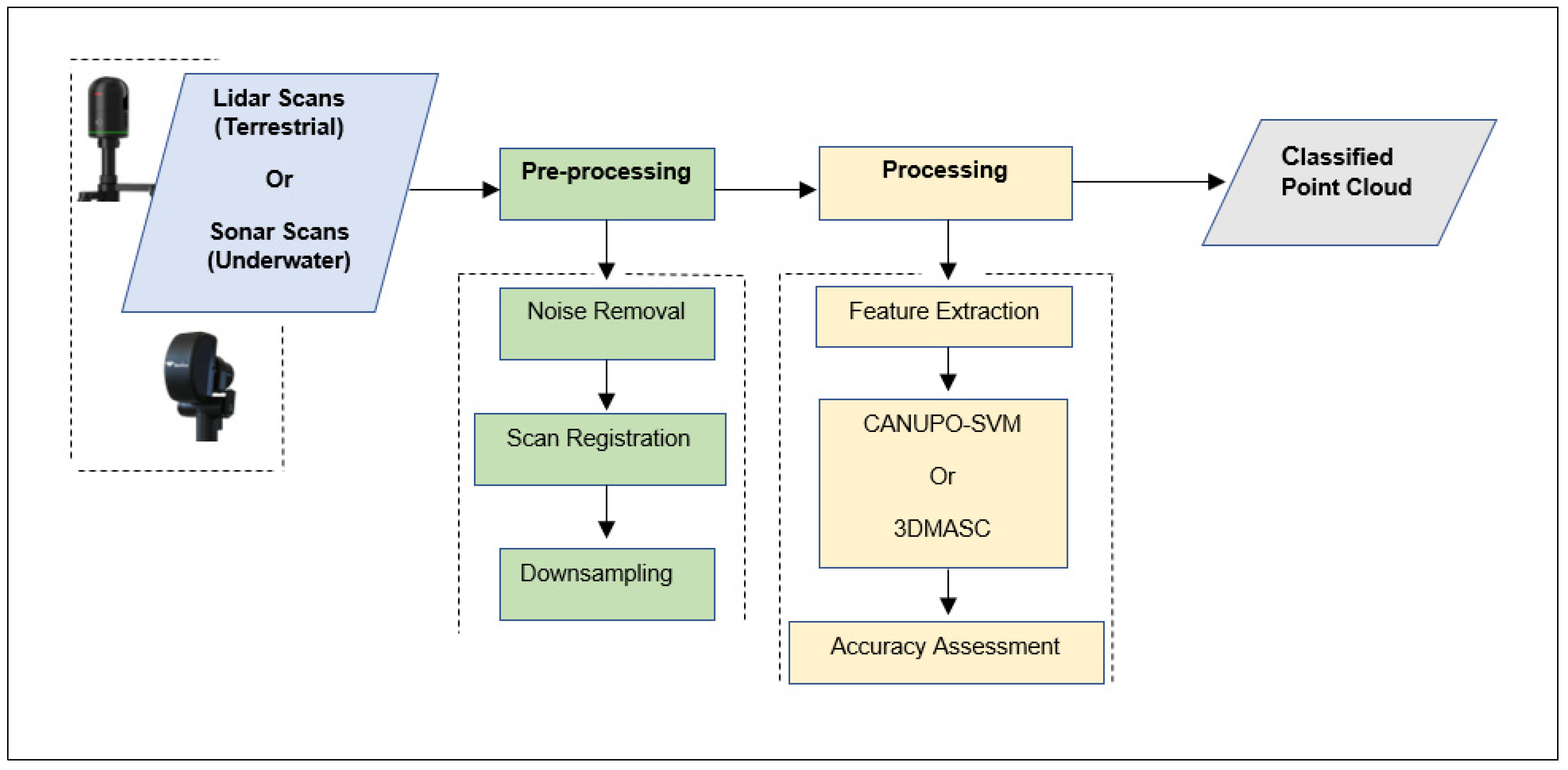
A structured methodological pipeline, summarised in Figure 1, was implemented in this study. The workflow comprised the acquisition of 3D point cloud data using terrestrial LiDAR and underwater acoustic scanning (sonar) systems. This was followed by data preprocessing, which included noise filtering, point cloud registration, and downsampling. Subsequent processing involved point cloud classification and accuracy assessment. Terrestrial and underwater point clouds were analysed both independently and in combination to support cross-domain experimentation. Finally, classification accuracy and related performance metrics were computed to evaluate classifier performance and generalisability across different sensing environments.

2.1. Materials

Plastic chairs and rubber tyres were chosen as target objects due to their clearly distinguishable geometric properties, enabling object-level analysis in both terrestrial and underwater domains. Tyres are dominated by curved, toroidal shapes, whereas chairs comprise planar and linear components, allowing the evaluation of contrasting morphological characteristics. These objects serve as simplified representations of common man-made structures encountered in marine environments, such as pipelines, anchors and structural components. 3D point cloud data was acquired using sensing technologies with fundamentally different signal characteristics. Terrestrial point cloud data was collected using a Leica BLK360 TLS based on LiDAR technology and designed by Leica Geosystems (Zuerich, Switzerland). The Leica BLK360 TLS operates on a time-of-flight (ToF) principle to produce high-resolution 3D point clouds [37]. LiDAR is a remote sensing technique used to determine distances by emitting pulsed laser radiation toward a target and detecting the returned signal. 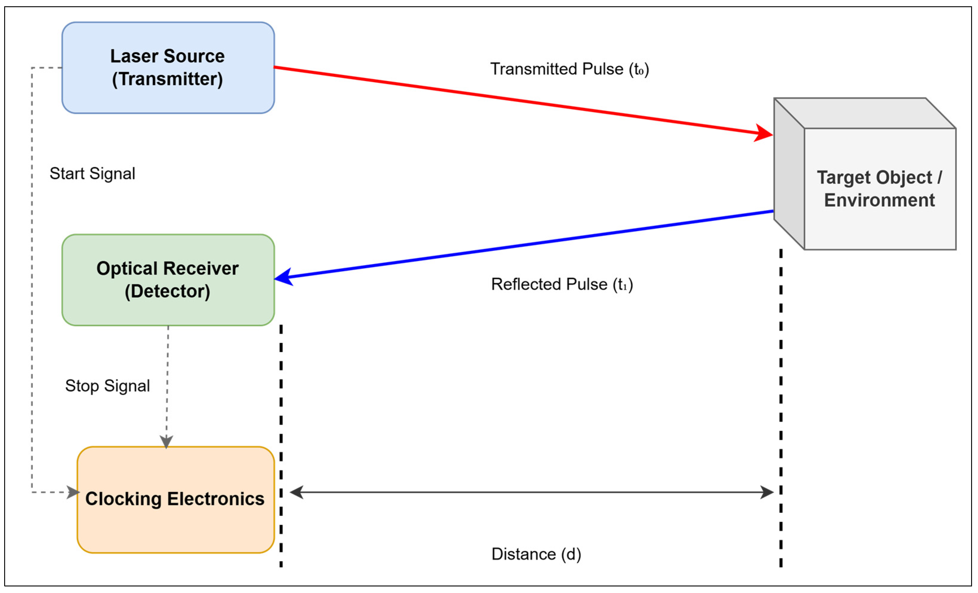Figure 2 illustrates the operating principle of ToF LiDAR. In this process, a laser transmitter emits short laser pulses in a specified direction. When the emitted beam interacts with an object, it is reflected or scattered according to the surface properties of the target. The returning echo is captured by the optical receiver and the distance between the sensor and the object is computed from the round-trip travel time of the laser pulse [37]. This ranging principle can be expressed using Equation (1), where d represents the distance to the target, c represents the speed of light and Δt represents the ToF (round-trip).

d = (c × Δt)/2,

(1)

Underwater point cloud data was acquired using a BlueView BV5000 mechanical scanning sonar (MSS) system developed by Teledyne Technologies (Thousand Oaks, CA, USA). Sonar is an active acoustic sensing method that uses sound wave propagation in aquatic environments for underwater ranging, spatial measurement, navigation and object detection [38]. The BV5000 emits fan-shaped acoustic signals and reconstructs object geometry from the returned echoes, thereby generating an underwater point cloud [39]. The principle of operation is similar to that of LiDAR, with the key difference being the use of acoustic waves instead of laser pulses. 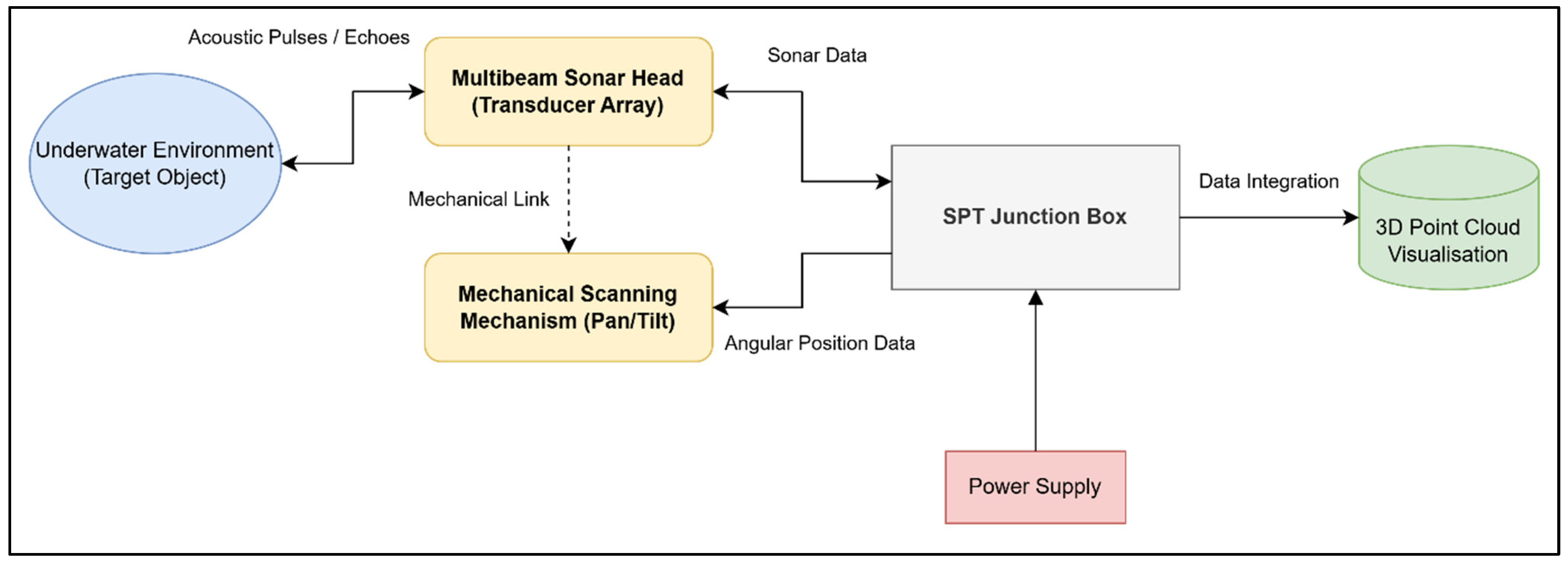Figure 3 shows the operational workflow of the BlueView MSS. The system emits acoustic pulses from the multibeam sonar head into the underwater environment, where echoes are returned from the target object and captured as sonar data. These data, together with angular position information from the mechanical scanning mechanism, are integrated via the junction box to generate a 3D point cloud for visualisation.

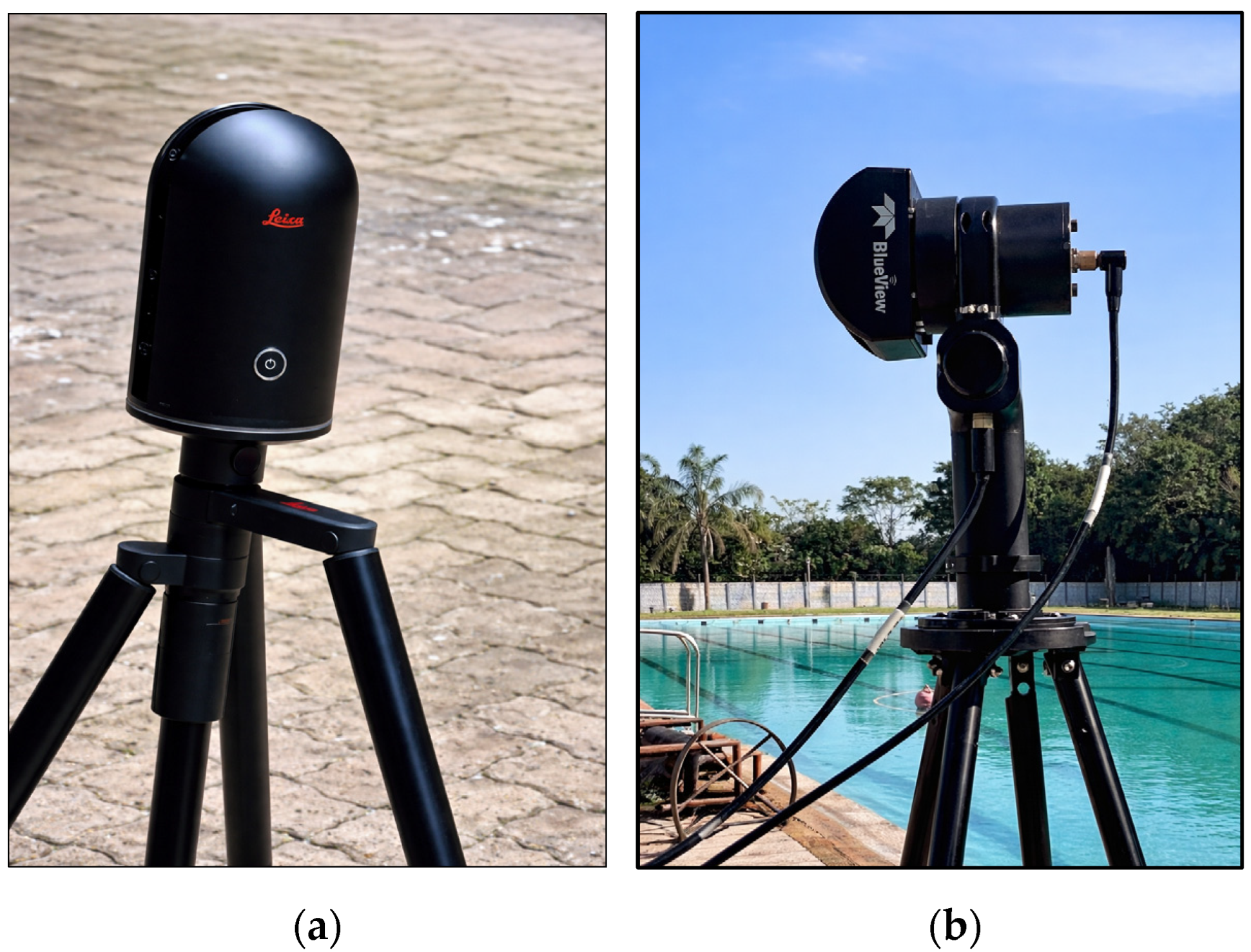
Figure 4 shows the Leica BLK360 and BlueView BV5000 MSS scanning systems used for terrestrial and underwater data acquisition, respectively. The specifications of the two aforementioned sensing systems used in this study are compared and summarised in

Table 1. Comparison of the Blueview BV5000 MSS and Leica BLK360 TLS specifications.

	Blueview BV5000 Sonar	Leica BLK360 TLS
Beam Width	1° × 1° (mm)	2.25 mm
Ranging error	15 mm	4 mm@10 m and 7 mm@20 m
Maximum Range	30 m	60 m
Horizontal resolution	~0.09° (16 mm@10 m)	3 (5/10/35 mm@10 m)
Vertical resolution	0.18° (30 mm@10 m)	3 (5/10/35 mm@10 m)
Field-of-view (vertical/horizontal)	45°/360° (320°/360°)	300°/360°

.

Point cloud datasets were processed using CloudCompare (version 2.13 Beta, www.cloudcompare.org) and Leica Cyclone Register 360 (version 2024.0.2) software for noise filtering, point cloud alignment, manual editing and classification. These platforms were selected for their capability to process large, high-density point clouds and to perform reliable registration and noise filtering.

2.2. Experimental Setup and Point Cloud Data Acquisition

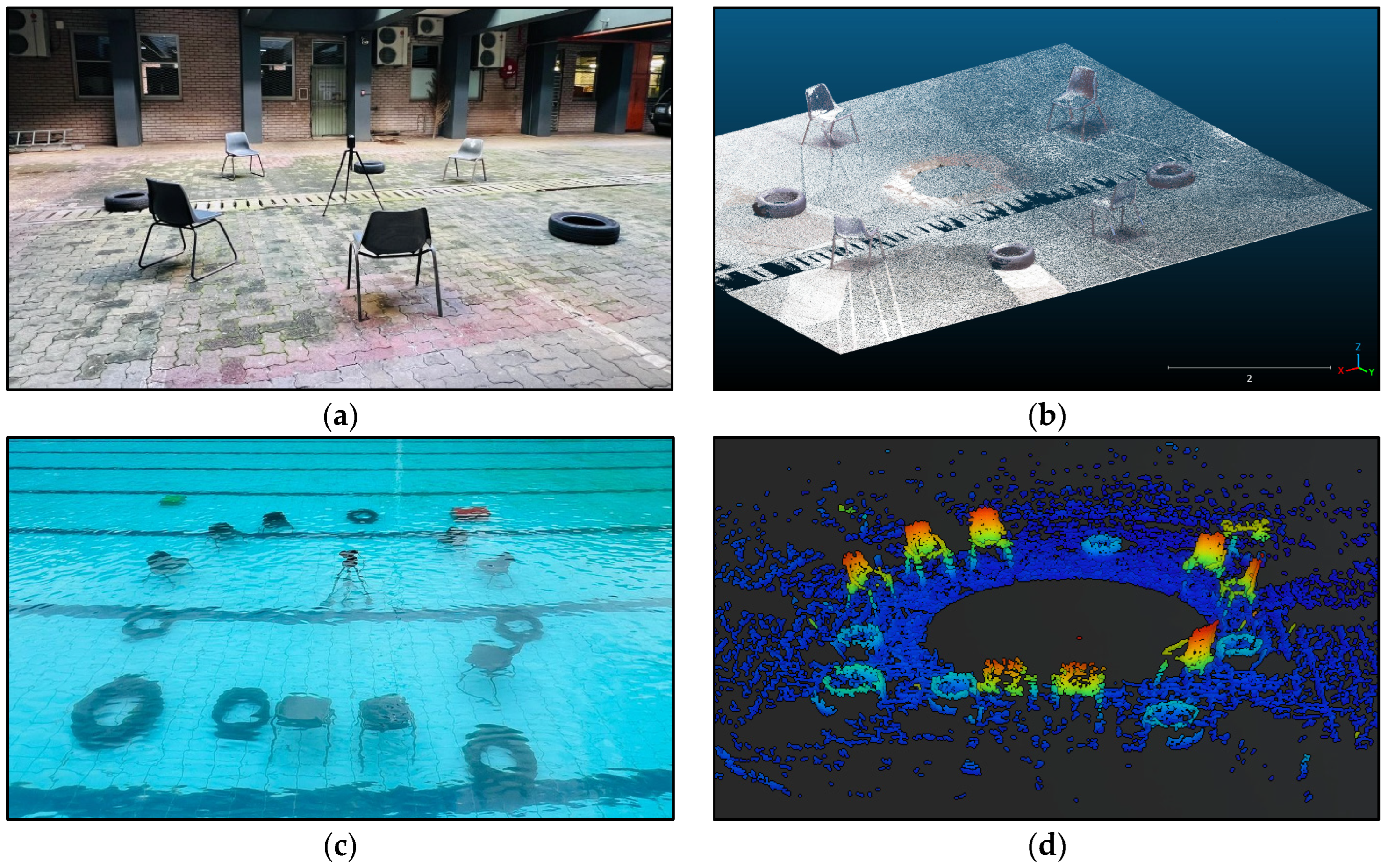
Controlled scanning sessions in both terrestrial and underwater environments were used to collect point cloud data. A similar scanning layout was maintained across both environments, with objects positioned in comparable orientations and at comparable distances from the scanner. A swimming pool was used as a controlled environment in which objects were submerged and scanned with a BV5000 MSS. Initially, image calibration was carried out to ensure measurement accuracy. All scans were acquired using consistent scanning settings, including single-return detection and spherical scanning with a 360° horizontal field of view and vertical angles of 0° and −15°. Where required by object geometry, an additional −45° vertical angle was used. Multiple scanner positions were employed to ensure complete 3D scene coverage. A similar setup was replicated for terrestrial data acquisition to ensure comparable object structure and scale across both sensing mediums. Terrestrial point cloud data were collected using a Leica BLK360 TLS in an open and stable environment. Objects were positioned at a fixed distance from the scanner, with consistent spacing and orientation maintained across all scans. Multiple scans were collected for each object to ensure sufficient spatial coverage of the dataset. 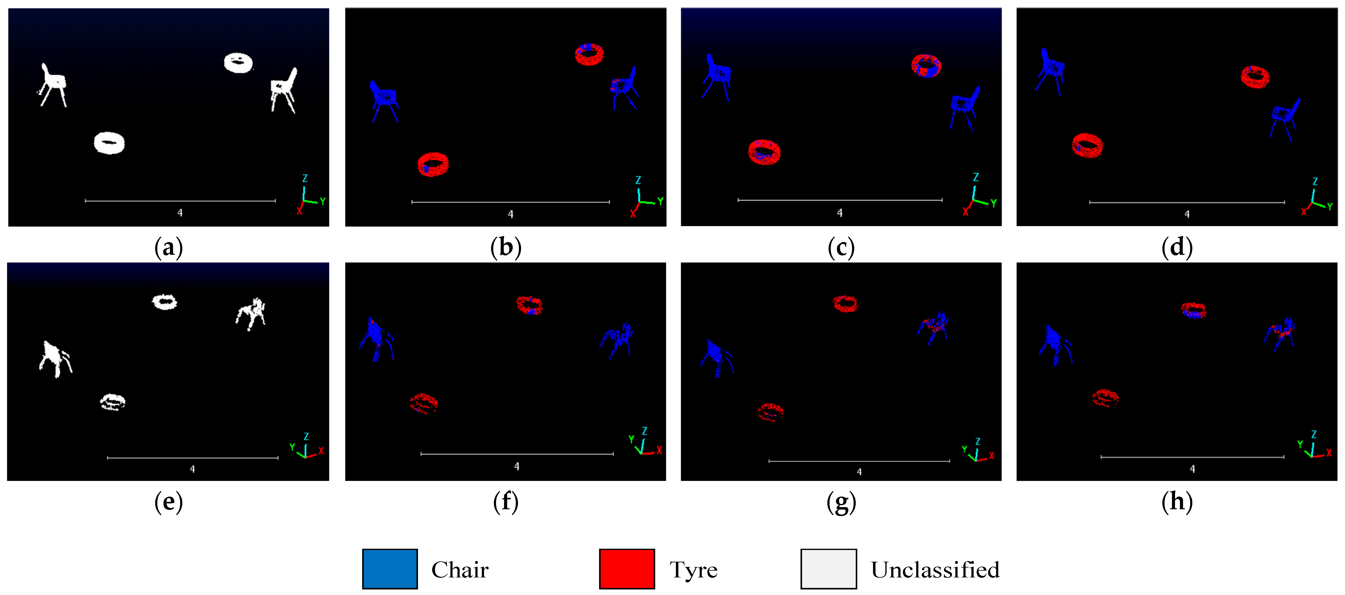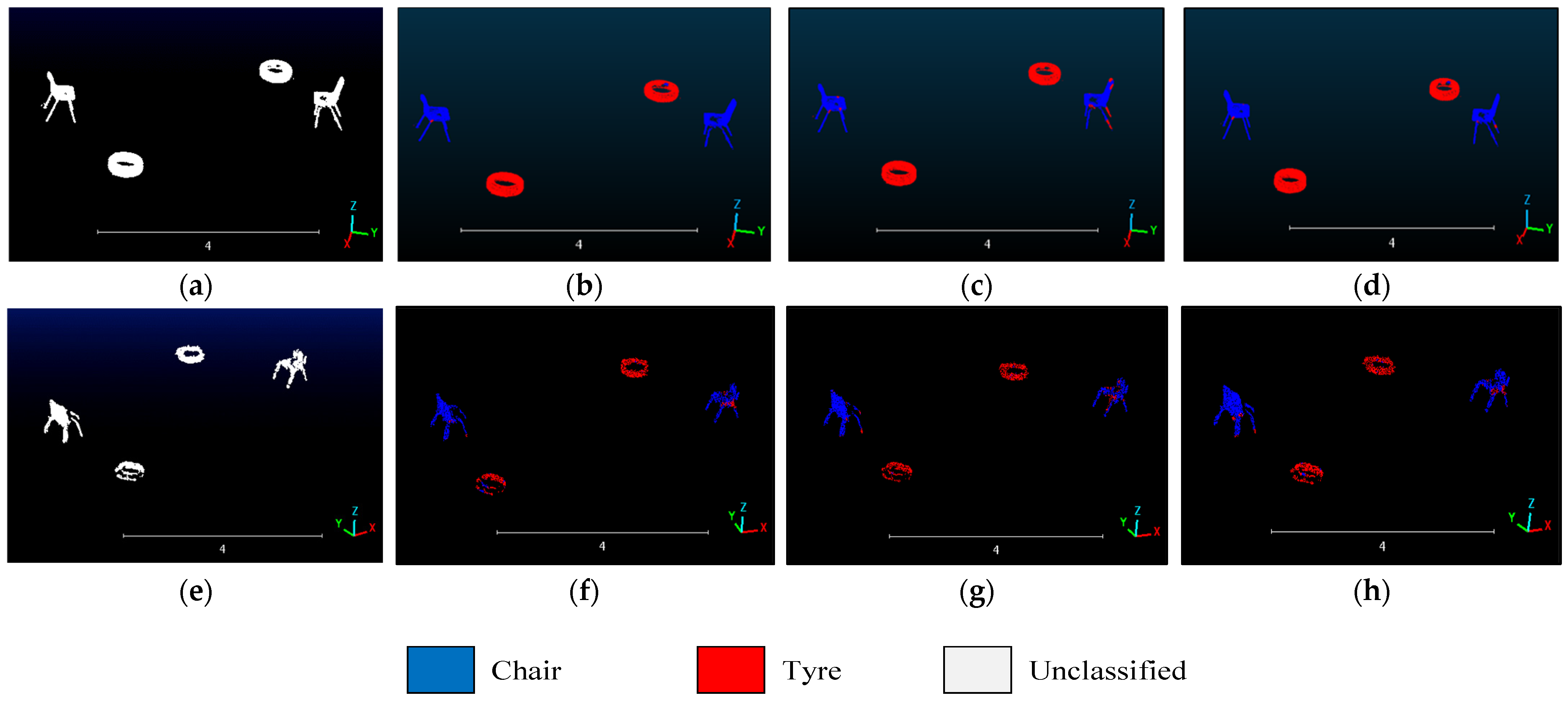Figure 5 presents the terrestrial objects and their corresponding LiDAR point cloud acquired with the Leica BLK360 TLS, along with the submerged objects and the sonar-derived point cloud collected with the Blueview BV5000 MSS.

2.3. Data Preprocessing

Point cloud preprocessing was performed using CloudCompare and Leica Cyclone 360. The software programs mentioned above provided essential tools for cleaning and registering the point cloud datasets. Noise and outliers were removed using a combination of manual segmentation and the automated cloth simulation filtering (CSF) algorithm [40]. This process was carried out separately for the terrestrial LiDAR and underwater acoustic datasets. After cleaning, the point clouds were registered to produce comprehensive, spatially coherent 3D representations of the environment. This was conducted independently for both the terrestrial and underwater datasets. Terrestrial LiDAR point clouds demonstrated higher resolution and geometric accuracy than underwater sonar data. LiDAR captured dense, detailed surface features with high definition. Sonar point clouds were smoother and less geometrically precise due to lower point density and acoustic effects such as multipath interference and signal attenuation. Multiple scans were registered and merged in CloudCompare to produce a common reference system.

2.4. Point Cloud Classification Algorithms

The Support Vector Machine (SVM) algorithm, introduced by Cortes and Vapnik [13], has become a widely adopted tool for both classification and regression tasks. It operates by applying a predefined non-linear mapping function that projects input vectors into a higher-dimensional feature space, within which a linear decision boundary with strong generalisation capabilities can be constructed. This approach allows the algorithm to identify an optimal hyperplane that not only separates classes but also maximises the margin between the closest points of opposing categories, referred to as support vectors in Boser et al. [41]. SVMs exhibit strong resistance to overfitting and perform well even when trained on relatively small datasets [42]. In this study, we applied the CAractérisation de NUages de POints (CANUPO) algorithm, a specialised SVM-based classifier designed by Brodu and Lague [25], to classify 3D point clouds. CANUPO characterises each point as 1D, 2D, or 3D based on local geometry across multiple scales. These descriptors form signatures from labelled data, which are projected to maximise class separability and define classification boundaries. Algorithm 1 outlines the procedure used in CloudCompare to perform CANUPO-SVM point cloud classification.

Algorithm 1. CANUPO-SVM point cloud classification

Input: Training point clouds; Validation point clouds; Training parameters Output: Classified point clouds 1.   Select samples for class #1 and class #2 from training data 2.   for (training): 3.    Specify multi-scale range; 4.    Select maximum core points; 5.    Train the CANUPO-SVM classifier; 6.    Evaluate class separability; 7.    if separability is not satisfactory then 8.        Adjust decision boundary; 9.     end if 10.   end for 11.   until separability is satisfactory; 12.   Save trained classifier; 13.   Load trained classifier; 14.   for each point in the validation dataset, do 15.    Apply classifier to assign class label 16.   end for 17.   for each predicted point, do 18.     Compare predicted label with ground truth 19.   end for 20.   Compute overall classification accuracy 21.   end

The second classification model used in this study is 3DMASC (Multiple Attributes, Scales, and Clouds), a supervised and explainable machine learning framework for 3D point cloud semantic classification [36]. The 3DMASC approach is designed to handle multiple point cloud attributes across different spatial scales and can integrate information from one or more point clouds. This makes it suitable for diverse datasets, including those with spectral and multi-return properties. Feature extraction is based on classical multi-scale geometric descriptors computed within spherical neighbourhoods or k-nearest neighbour regions, following established dimensionality-based methods [25]. These descriptors capture object shape characteristics such as linearity, planarity, sphericity, and eigenvalue ratios, derived through principal component analysis (PCA) of local point distributions. ZRANGE represents the vertical extent of the neighbourhood, calculated as the difference between the maximum and minimum elevation values. 3DMASC classification is performed using a RF algorithm, which constructs an ensemble of decision trees from bootstrap samples to improve prediction accuracy and robustness [14]. At each split, a random subset of features is selected to reduce overfitting and introduce diversity among trees [43]. The final class label is determined through majority voting across the forest. This provides insight into which features are most influential for classification. The 3DMASC implementation in CloudCompare also requires a parameter file defining the spatial scales at which descriptors are computed, enabling systematic feature fusion and improved classification performance. Algorithm 2 outlines the workflow used in CloudCompare to perform 3DMASC point cloud classification.

Algorithm 2. 3DMASC point cloud classification

Input: Training point clouds; Validation point clouds; Parameter file Output: Classified point clouds 1.   Load the Parameter file; 2.   Select features to be considered for training; 3.   for (training): 4.       Define Random Trees parameters (maximum depth, number of trees, minimum       sample count); 5.       Train the classifier; 6.       Evaluate training results; 7.         if results are not satisfactory then 8.           Modify feature selection; 9.         end if 10.   end 11.   until results are satisfactory; 12.   Save trained classifier; 13.   Load saved classifier; 14.   for each point in the validation dataset, do 15.         Apply classifier to assign class label; 16.   end for 17.   for each predicted point, do 18.         Compare predicted label with ground truth; 19.   end for 20.   Compute overall classification accuracy; 21.  end

2.5. Implementation

In this study, three distinct point cloud datasets were prepared. The first dataset comprised terrestrial data acquired through the Leica BLK 360 TLS. The second dataset included only the underwater data generated using the Blue View BV5000 MSS. Lastly, the third dataset was a combined point cloud consisting of merged terrestrial and underwater point clouds. Prior to classification, all datasets underwent preprocessing in CloudCompare, including noise filtering, removal of irrelevant surfaces and point cloud registration to ensure geometric alignment. Additionally, all datasets were annotated in CloudCompare, where points were manually labelled into two object classes: chairs and tyres. Conventional machine learning practices typically recommend a 70:30% split between training and validation sets. However, both CANUPO-SVM and 3DMASC classification algorithms deliver reliable performance even with relatively small training samples when informative geometric descriptors are used.

For CANUPO-SVM classification, a maximum of 10,000 core points were used for training, with spatial scales ranging from 0.1 m to 1.0 m, and point dimensionality was selected as the primary classification attribute. Classifiers were intentionally trained and evaluated using unnormalised terrestrial and underwater point clouds. This was conducted in order to assess the inherent robustness of the CANUPO-SVM framework when applied to heterogeneous datasets. The decision to work with unnormalised data reflects real-world operational scenarios. In reality, variations in scale and density are common due to differences in sensor characteristics and environmental conditions. This approach allows for a realistic evaluation of the classifier’s generalisation capability and its potential for deployment in applications where preprocessing is impractical or infeasible.

Model generalisability and transferability were evaluated using three training configurations: training on terrestrial data only, training on underwater data only, and training on a combined dataset comprising both terrestrial and underwater samples. Each trained classifier was then applied independently to both terrestrial and underwater data to evaluate its performance under matched and mismatched domain conditions. This multi-scenario framework enabled a comprehensive assessment of CANUPO-SVM’s classification accuracy, cross-domain robustness and transferability in the context of 3D point cloud data.

For 3DMASC classification, similar datasets were used during training to evaluate intra-domain and cross-domain performance. The 3DMASC tool in CloudCompare requires a parameter file specifying the spatial scales and geometric descriptors used for training. An ablation-style parameter selection was conducted by testing different feature–scale combinations, after which the optimal configurations were retained. A consistent 70:30% training–testing split was applied, with labelled chair and tyre samples used for supervised learning. Three 3DMASC RF classifiers were trained under different domain configurations. Classifier 1 was trained on terrestrial LiDAR using descriptors at scale SC1. Classifier 2 was trained on underwater sonar using multi-scale descriptors (SC0.4 and SC1), including ZRANGE. Classifier 3 was trained on the combined dataset using the same multi-scale feature set. The selected descriptors and scales are summarised in

Table 2. Parameter configuration of the 3DMASC classifiers used in this study.

Classifier	Training Domain	Spatial Scales	Geometric Descriptors
Classifier 1	Terrestrial	SC1.0	PCA2, PCA3, Planarity, Sphericity, Linearity
Classifier 2	Underwater	SC0.4, SC1.0	PCA2, PCA3, Planarity, Sphericity, Linearity, ZRANGE
Classifier 3	Combined	SC0.4, SC1.0	PCA2, PCA3, Planarity, Sphericity, Linearity, ZRANGE

. RF hyperparameters were tuned with maximum depth = 20, tree count = 10 and minimum sample count = 15. Although RF models are generally robust to moderate class imbalance, class distributions were monitored to ensure adequate representation of both object classes. Each trained classifier was subsequently applied to both terrestrial and underwater test data to assess classification robustness and transferability across sensing environments.

2.6. Evaluation Metrics and Classifier Performance

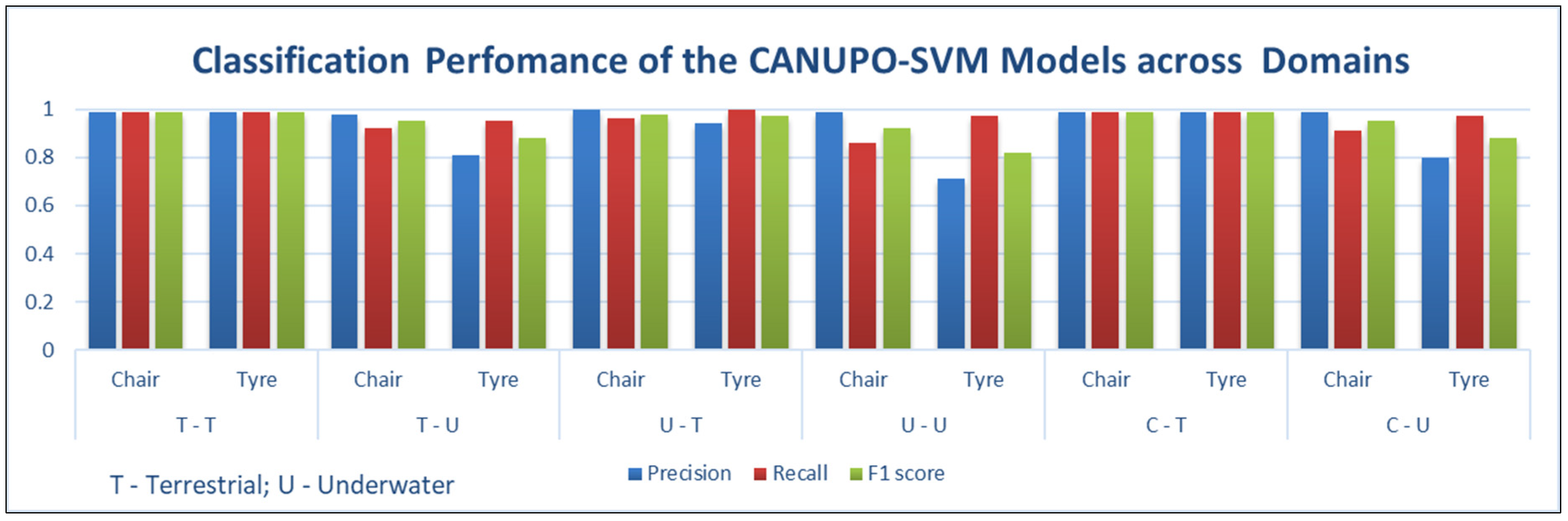
The evaluation of point cloud classification performance was conducted using a set of well-established statistical metrics derived from the confusion matrix. This matrix provides a detailed account of classifier predictions by comparing the actual object class labels with the model’s predicted labels. It identifies true positives (TP), true negatives (TN), false positives (FP) and false negatives (FN), which form the basis for computing performance indicators. Four key statistical indicators were calculated: accuracy, precision, recall and the F1 score. These metrics collectively provide a comprehensive picture of the model’s classification abilities. Accuracy measures the overall proportion of correctly classified points and reflects the model’s ability to assign the correct label across all classes (Equation (2)). Precision quantifies the accuracy of positive predictions made by the classifier (Equation (3)). Recall (sensitivity) quantifies the proportion of actual positive points that are correctly identified as true positives (Equation (4)). The F1 score combines precision and recall through their harmonic mean (Equation (5)). The accuracy indicators described above are calculated as follows:

Accuracy = (TP + TN)/(TP + TN + FP + FN)

(2)

Precision = TP/TP + FP

(3)

Recall = TP/TP + FN

(4)

F1 score = 2 × (Recall × Precision)/(Recall + Precision)

(5)

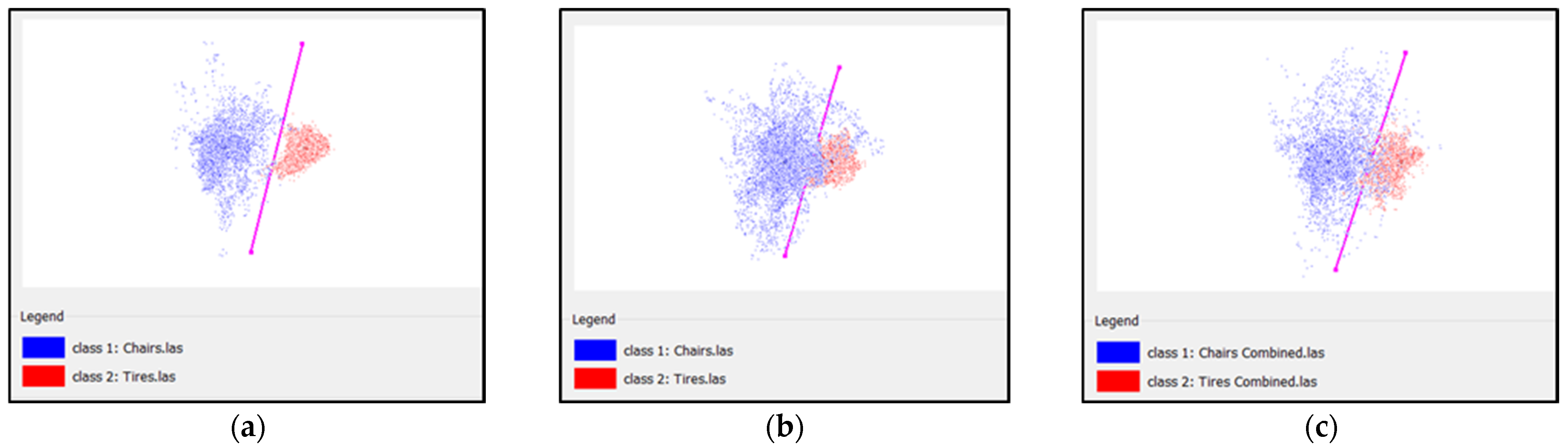
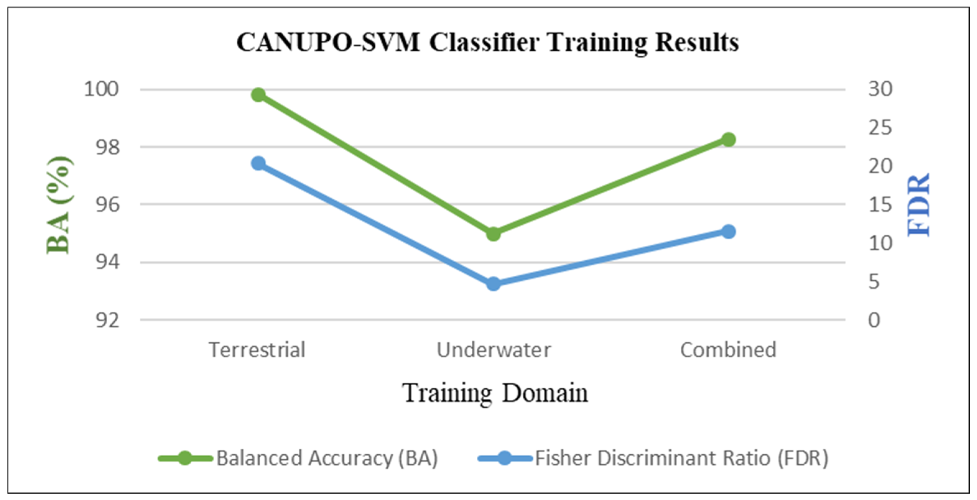
The CANUPO–SVM training phase provided insight into both classification accuracy and class separability. Classification performance is quantified using balanced accuracy (BA), while the degree of separation between feature classes is assessed using the Fisher Discriminant Ratio (FDR). BA (Equation (7)) is derived from recall and selectivity (Equation (6)) [44]. Higher BA values indicate stronger recognition capability, whereas higher FDR values reflect clearer separation between classes in the feature space. The FDR is calculated using Equation (8), where the mean (μ_c) and variance (v_c) of the signed distance to the SVM decision boundary are computed for each class, allowing an objective evaluation of feature separability during training [25].

Selectivity = TN/TN + FP

(6)

Balanced Accuracy = (Recall + Selectivity)/2

(7)

FDR = (μ₂ − μ₁)²/(v₁ − v₂)

(8)

3. Results

All experiments were performed in the CloudCompare environment on a 64-bit machine with an Intel Core i7 CPU and 16 GB of RAM. Computational performance was evaluated in terms of training and inference durations. For CANUPO SVM, training durations ranged from 17 s to 2 min, while 3DMASC required longer training times ranging from 51 s to 18 min. Inference durations for CANUPO SVM varied between 4 s and 2 min depending on the domain configuration, whereas 3DMASC achieved consistently lower inference times between 3 and 20 s. The results are organised into classifier training and validation outcomes. Classification performance is reported for intra-domain, cross-domain, and combined-domain scenarios. Both visual and quantitative analyses are used to assess feature separability, classification performance, and cross-domain generalisation across terrestrial and underwater environments.

3.1. CANUPO-SVM Training

The classifier training results demonstrate clear differences in feature separability across the three training configurations. Figure 6 illustrates the distribution and separation of feature classes obtained when the CANUPO–SVM classifier was trained on terrestrial, underwater and combined datasets, respectively. In the terrestrial training scenario (Figure 6a), the feature classes are clearly separated with the SVM identifying a clear decision boundary that maximises class separation. This is shown by a high BA of 0.9984 and an FDR of 20.3378. Training on underwater data (Figure 6b) results in reduced but still observable separability with a BA of 0.9500 and an FDR of 4.6491. When terrestrial and underwater samples are combined during training (Figure 6c), the classifier maintains consistent separability, obtaining a BA of 0.9827 and an intermediate FDR of 11.5863. The corresponding BA and FDR values are summarised in Figure 7, allowing direct comparison among the three training configurations. Overall, the training results indicate strong and stable feature separation across all datasets. All the trained classifiers were saved for further application to unseen 3D point cloud datasets during the validation or testing phase.

3.2. 3DMASC Training

The 3DMASC RF classifiers showed stable and reliable training performance across all training settings. Training was conducted using a 70:30 data split, with 30% of the samples reserved for classifier internal validation. The RF parameters (10 trees; maximum depth 20) were selected empirically during tuning and retained because validation performance was consistent across training configurations. When trained on terrestrial data, the model achieved an overall accuracy of 99%. Training on underwater data resulted in a slightly lower overall accuracy of 97%. When terrestrial and underwater samples were combined during training, the classifier again achieved an overall accuracy of 99%.

3.3. Classifier Validation

In this study, the experimental procedure was structured into three phases to evaluate classification performance and cross-domain generalisation between terrestrial and underwater point cloud data. The following scenarios were systematically evaluated:

• Training and testing within a single sensing modality (terrestrial–terrestrial and underwater–underwater);
• Training on one modality and testing on the other (terrestrial–underwater and underwater–terrestrial);
• Training on a combined terrestrial and underwater dataset, followed by independent testing on each modality.

Both CANUPO–SVM and 3DMASC RF classifiers were validated on terrestrial and underwater point cloud datasets. Classifiers trained under different configurations were applied to independent validation sets, with irrelevant surfaces removed beforehand to reduce background influence, especially for CANUPO–SVM. Classification results were presented visually and evaluated quantitatively using standard performance metrics. Figure 8 presents a visual overview of the CANUPO–SVM classification results across different training and testing configurations. To complement the visual assessment shown in Figure 8, a quantitative evaluation of classification performance was conducted using the standard performance metrics, as presented in Figure 8 and

Table 3. Overall classification accuracy of the CANUPO–SVM and 3DMASC–RF classifiers across intra-domain, cross-domain, and combined-domain training and testing configurations.

Domain	CANUPO-SVM	3DMASC
terrestrial–terrestrial	0.99	0.97
terrestrial–underwater	0.93	0.95
underwater–underwater	0.97	0.86
underwater–terrestrial	0.89	0.95
combined–terrestrial	0.99	0.99
combined–underwater	0.93	0.84

. Figure 9 shows a graphical presentation of the precision, recall and F1-score obtained by the CANUPO–SVM classifier across terrestrial, underwater and combined training and testing domain configurations. The corresponding overall accuracies are provided in Table 3.

When the terrestrially trained classifier was applied to the terrestrial validation dataset, excellent results were obtained, as shown in Figure 8b. An overall accuracy of 99% was achieved. Figure 8f shows the results obtained when the same classifier was applied to an underwater point cloud, the accuracy dropped to 93%. This accuracy drop was expected since the classifier was trained in a different environment. However, these results indicate that the CANUPO-SVM classifier has good generalisation ability to a different unseen environment. Misclassifications are evident in Figure 8f: some points were assigned to incorrect categories. The classifiers were also trained using the samples from the underwater point cloud. Figure 8g shows the results obtained when the underwater-trained classifier was applied to the underwater test data, achieving an accuracy of 97%. Figure 8c shows the results obtained when the same classifier was then applied to the terrestrial point cloud. An overall accuracy of 89% was achieved, demonstrating a reduction in performance under cross-domain conditions. Following assessment of intra- and cross-domain generalisation, the training samples from both terrestrial and underwater datasets were merged and subsequently evaluated in each domain independently. Figure 8d and Figure 8h present the classification results obtained using the combined training configuration for the terrestrial and underwater domains, respectively. In this case, the classifier achieved an overall accuracy of 99% on the terrestrial test set and 93% on the underwater test set, indicating improved performance across both environments compared with single-domain training.

The 3DMASC RF classification performance was also assessed in the same manner. Figure 10 shows the classification results obtained when the 3DMASC RF classifiers were applied to unseen terrestrial and underwater point cloud test data. The corresponding performance indicators are graphically presented in Figure 11, showing precision, recall, and F1 Scores, while the classification accuracies are presented in Table 3.

Figure 10b shows the classification results obtained when the classifier was trained and tested within the terrestrial domain. An excellent performance was observed with an overall accuracy of 97%. Applying the same terrestrially trained classifier to underwater validation data yielded 95% accuracy, indicating a moderate reduction under cross-domain conditions (see Figure 10f). These results demonstrate that the 3DMASC classifier maintained high performance when transferred from terrestrial to underwater environments.

The underwater-trained classifier showed more variable behaviour. When applied to underwater validation data, an overall accuracy of 86% was achieved, reflecting increased complexity within the submerged dataset (see Figure 10f). However, when the same classifier was applied to terrestrial data, performance improved, achieving 95% accuracy (see Figure 10c). The results show that models trained on underwater data transfer more effectively to terrestrial datasets than models trained on terrestrial data transfer to underwater datasets. The classification results for the combined training configuration are presented in Figure 10d and Figure 10h for the terrestrial and underwater domains, respectively. In this configuration, the 3DMASC classifier achieved an overall accuracy of 99% on the terrestrial test set and 84% on the underwater test set, as summarised in Table 3. Compared with single-domain training, these results show improved, more consistent performance on terrestrial data, while classification accuracy in the underwater domain remained comparatively lower.

As shown in Table 3, both CANUPO–SVM and 3DMASC models performed strongly in terrestrial-to-terrestrial classification, with CANUPO–SVM slightly higher. In terrestrial-to-underwater transfer, 3DMASC achieved better accuracy than CANUPO–SVM. Underwater-to-underwater experiments showed stronger performance for CANUPO–SVM, whereas 3DMASC achieved lower accuracy. In underwater-to-terrestrial transfer, 3DMASC again outperformed CANUPO–SVM. Combined-domain training produced equal results for terrestrial testing, whereas CANUPO–SVM remained higher than 3DMASC for underwater testing.

The F1-scores further clarify cross-domain underwater performance, as presented in

Table 4. F1-scores for cross-domain underwater transfer.

Domain	Object	CANUPO-SVM	3DMASC
terrestrial–underwater	Chair	0.99	0.97
	Tyre	0.93	0.95
combined–underwater	Chair	0.99	0.99
	Tyre	0.93	0.84

. In the terrestrial-to-underwater transfer scenario, both classifiers achieved identical F1-scores of 0.95 for chair detection, indicating strong object separability across sensing modalities. For tyre detection, 3DMASC achieved a higher F1-score (0.94) than CANUPO (0.88), indicating improved classification precision and recall under underwater conditions. The combined-domain training configuration provides additional insight into multi-environment learning behaviour. In the combined-to-underwater scenario, CANUPO maintained stable performance, achieving F1-scores of 0.95 for chairs and 0.88 for tyres. Conversely, 3DMASC performance declined to 0.86 and 0.82 for chairs and tyres, respectively, indicating reduced classification consistency under mixed-domain training.

4. Discussion

The analysis focused on two classical frameworks, CANUPO–SVM and 3DMASC–RF. In this work, generalisation refers to reliable model performance on unseen data within the same sensing domain. Transferability describes the ability of a model trained in one environment to operate on a different modality without retraining. Together, these concepts provided a clear basis for assessing both intra-domain and cross-domain applicability. Classification performance was also evaluated under combined-domain conditions, in which the source and target datasets were jointly used during training to assess integrated learning stability. Previous studies have treated mainly terrestrial and underwater semantic classification as separate problems, with most methods developed for single-domain applications. Although domain adaptation and transfer learning models exist, they focus on terrestrial environments. In contrast, this study examines adaptation-free transfer, enabling the observed performance differences to be directly attributed to feature-space behaviour rather than domain alignment mechanisms.

The performance within the same domain confirms strong feature class consistency within each domain. Both classifiers show high accuracy when trained and tested within the same domain. The terrestrial–terrestrial evaluation achieved accuracies of 0.99 for CANUPO–SVM and 0.97 for 3DMASC. Similar levels of performance have been reported in previous terrestrial LiDAR classification studies, where SVM and RF classifiers have been applied [45,46,47]. These results demonstrate that the handcrafted geometric features employed by both approaches are strongly discriminative in terrestrial LiDAR environments. The consistent point density and stable surface structure of terrestrial LiDAR scans support this strong performance. In the underwater–underwater scenario, CANUPO–SVM maintained a high accuracy of 0.97, whereas 3DMASC decreased to 0.86. This suggests that CANUPO’s dimensionality-based representation is more robust under sonar acquisition, while 3DMASC is more sensitive to underwater data variability. The reliance on basic geometric structures makes CANUPO robust to sonar noise, while 3DMASC’s complex features are more affected by underwater data variability. Similar performance trends have been reported in underwater machine learning classification studies where sonar point clouds were classified using feature-based approaches [48,49].

Under cross-domain evaluation, both classifiers showed performance reductions due to domain shift between LiDAR and sonar point clouds. Differences in point density, acquisition geometry and noise characteristics primarily drive this shift. CANUPO–SVM achieved an accuracy of 0.93 in the terrestrial-to-underwater transfer but declined to 0.89 in the underwater-to-terrestrial scenario, indicating sensitivity and modality-dependent feature patterns. In contrast, 3DMASC maintained a consistent cross-domain accuracy of 0.95 in both transfer directions, reflecting more stable generalisation associated with the ensemble and non-linear structure of RF learning. However, its lower intra-underwater accuracy (0.86) highlights the increased geometric variability and reduced structural consistency inherent in submerged point clouds. These results support recent trends showing that multiscale feature modelling and feature-space aggregation enhance generalisation with classical frameworks achieving this through geometric descriptors. However, the stability of cross-domain transfer is strongly dependent on hyperparameter selection, particularly the choice of multi-scale neighbourhood sizes. Small neighbourhoods are more sensitive to sonar noise and sparsity, while larger neighbourhoods may oversmooth object geometry and reduce class separability by incorporating background structures. Combined-domain training was further assessed by integrating the source and target datasets into a single learning setup. Both classifiers performed strongly on terrestrial samples, achieving accuracies of 0.99 (CANUPO–SVM) and 0.99 (3DMASC). For underwater validation, CANUPO retained an accuracy of 0.93, while 3DMASC dropped to 0.84, indicating that it remains more affected by the greater structural variability present in submerged environments. This behaviour highlights how mixed-domain training introduces heterogeneous feature distributions, where dimensionality-based descriptors exhibit greater resilience, while multi-feature learning remains sensitive to increased variance across sensing modalities.

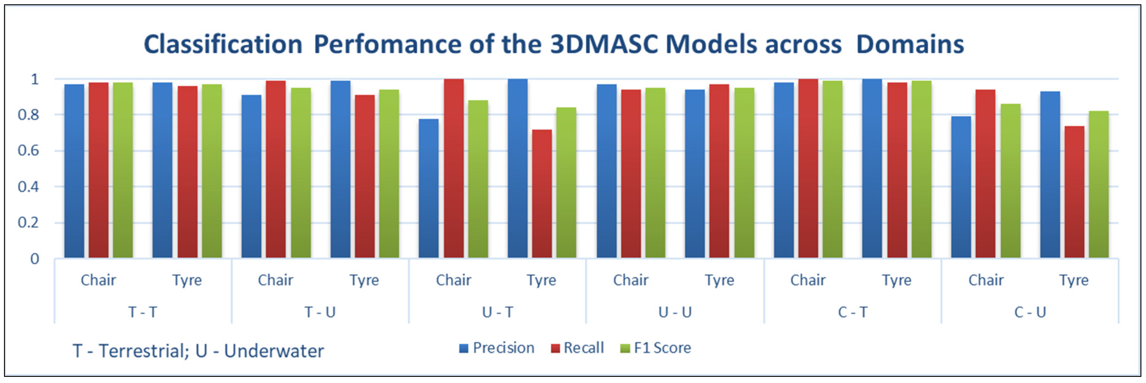
F1-scores provide further insight into cross-domain classification behaviour. Consistently high detection accuracy indicates that objects with simple planar geometry remain strongly separable despite cross-sensor differences, as supported by BA and FDR trends. Higher performance by 3DMASC in the terrestrial-to-underwater transfer reflects the advantage of multi-scale feature modelling. However, its performance declined under combined-domain training, suggesting sensitivity to mixed-domain feature heterogeneity. CANUPO demonstrated more stable generalisation across integrated datasets, while misclassification was primarily influenced by sonar noise, shadowing, and density variation. Overall, the results highlight the influence of training domain composition and scale sensitivity on cross-domain classifier transferability.

During the 3DMASC implementation, ablation experiments were conducted to assess the influence of individual features. The ZRANGE descriptor was found to have high feature importance, and its removal in the combined-domain scenarios led to a significant drop in classification accuracy. This confirms that vertical range information is essential for robust feature discrimination and stable generalisation across sensing modalities. In contrast, CANUPO–SVM relies on multi-scale dimensionality-based descriptors, suggesting that the geometric separability of the target objects across domains mainly drives its transferability. While strong results were achieved, the experiments were based on relatively small, controlled datasets acquired directly from the sensors. This limits large-scale statistical generalisation to more diverse real-world environments. In addition, the analyses focused on only two object classes, while background surfaces, such as the floor, were removed prior to classification. This preprocessing was necessary to ensure a reliable evaluation and to accommodate the binary nature of the CANUPO–SVM framework, allowing the classifiers to focus on the target objects. Retaining background elements would increase geometric complexity and competing features, likely reducing accuracy and increasing false positives. It would also raise processing time, particularly for 3DMASC due to its iterative training process. In practical marine environments, objects such as pipelines, anchors and structural elements exhibit linear, cylindrical or planar geometries similar to those used in this study. These can be approximated in terrestrial settings, enabling controlled and repeatable data acquisition. Terrestrial surveys are also more cost-effective and easier to conduct than underwater surveys. In real underwater environments, clutter, uneven seabeds and partial burial may reduce class separability and increase misclassifications, especially for geometry-based classifiers.

The experiments were conducted on simple objects in a controlled swimming pool environment. The limited dataset and lack of environmental complexity such as turbidity and natural clutter may reduce generalisation to real underwater scenarios. Nevertheless, these results provide a proof-of-concept for cross-domain classification and indicate potential for real-world applications. Another limitation is that the study focused exclusively on classical machine learning classifiers rather than deep learning approaches. This was intentional, as the primary objective was to assess the transferability and interpretability of feature-based methods under limited training data conditions, which are common in both terrestrial and underwater point cloud applications. The cross-domain behaviour observed in this study indicates that dimensionality-based descriptors capture stable geometric structures that remain meaningful across different sensing modalities. Despite fundamental differences between terrestrial LiDAR and underwater sonar point clouds, these geometric representations preserve object-level separability under modality shifts. This suggests that training on geometrically representative terrestrial proxies can provide an efficient preliminary step, especially where labelled sonar data are limited or costly to obtain.

Furthermore, the recorded computational durations provide quantitative evidence that both CANUPO-SVM and 3DMASC are computationally efficient classical machine learning classifiers. CANUPO-SVM exhibits faster training but shows greater variability during inference, particularly for terrestrial datasets. In contrast, 3DMASC requires longer training durations but delivers faster and more stable inference. Overall, the findings demonstrate that classical geometric machine learning models can transfer effectively between terrestrial and underwater environments. Dimensionality-based features provide consistent structural information across domains while remaining computationally efficient, requiring fewer training samples and lower processing resources than deep learning approaches.

5. Conclusions

The main aim of this study was to evaluate the cross-domain generalisability of classical geometric machine learning classifiers between terrestrial LiDAR and underwater sonar point clouds, including classification scenarios that use combined source and target training data. A structured workflow was implemented using multi-scale feature extraction and supervised classification under intra-domain, cross-domain, and combined-domain scenarios. Two dimensionality-based frameworks, CANUPO–SVM and 3DMASC–RF, were assessed to determine whether models trained in one sensing environment could operate reliably in another without retraining. The results demonstrate that dimensionality descriptors capture stable geometric structures across sensing modalities. Strong classification performance was achieved within individual domains, confirming reliable feature separability. Cross-domain transferability was also achieved, though performance decreased. Combined-domain training further demonstrated that integrating source and target datasets can enhance classification stability, particularly within terrestrial evaluations, while underwater performance remained influenced by structural variability.

From an operational perspective, the findings support unified classification workflows for integrated land–water semantic mapping applications. These include coastal infrastructure monitoring, submerged object detection, and digital twin development. Classifier transfer reduces the need for separate training pipelines and extensive manual annotation. In addition, classical geometric models remain computationally efficient. They require fewer training samples and lower processing resources than deep learning approaches, making them suitable for data-scarce environments. Future research should extend validation to larger multi-class datasets and more complex underwater scenes. Comparative benchmarking with deep learning frameworks and investigation of domain adaptation strategies will further improve cross-domain robustness and operational applicability.