A Two-Stage Semiempirical Model for Satellite-Derived Bathymetry Based on Log-Ratio Reflectance Indices

Abstract

Accurate bathymetric information is crucial for coastal management, navigation, and ecosystem monitoring, yet conventional hydrographic surveys are costly and logistically demanding. This study introduces a two-stage semiempirical model for satellite-derived bathymetry (SDB) based on log-ratio reflectance indices from atmospherically corrected Landsat 8 imagery. The approach combines the optical sensitivity of the green/blue band ratio and the attenuation properties of the red/blue ratio within a parametric regression framework, enhancing both stability and interpretability. The methodology was evaluated in two contrasting coastal environments: the turbid Magdalena-Almejas Lagoon System (Mexico) and the clear-water coral reef setting of Buck Island (U.S. Virgin Islands). Results demonstrated that the proposed model outperformed traditional semiempirical approaches (Lyzenga, Stumpf, Hashim), achieving $R^2=0.8155$ (RMSE = 1.16 m) in Magdalena-Almejas and $R^2=0.9157$ (RMSE = 1.38 m) in Buck Island. Performance was statistically superior to benchmark methods according to cross-validated confidence intervals and was comparable to an artificial neural network, while avoiding overfitting in data-scarce environments. These findings highlight the model’s suitability as a transparent, cost-efficient, and scalable alternative for SDB, particularly valuable in regions where in situ data are limited.

1. Introduction

Coastal bathymetry is essential for managing ecosystems, planning infrastructure, and supporting economic activities such as fisheries, navigation, and tourism. However, traditional hydrographic surveys are costly and logistically challenging in shallow or turbid waters. Satellite-derived bathymetry (SDB) has emerged as a practical and cost-efficient alternative, offering repeatable and large-scale coverage for dynamic coastal environments [1,2].

Over the past decades, several semiempirical models have been widely adopted to estimate bathymetry from multispectral imagery. Lyzenga proposed a log-linear approach to account for light attenuation in water [3], Stumpf introduced a band-ratio model that relies on the ratio of logarithms of reflectance bands [4] while Hashim proposed the use of various bathymetry algorithms, including Single-Band Algorithm (SBA) and Green-Band Algorithm (GBA), along with Principal Component Analysis (PCA) and the SPEAR Relative Water Depth tool from ENVI [5]. These strategies remain popular due to their transparency and relatively low data requirements, although their accuracy is limited in certain environmental conditions [6,7].

Table 1. Summary of commonly used semiempirical methods.

Method	Equations	Constants	Variables
Lyzenga	$\mathrm{Z}=a_0+{\sum }_{i=1}^N{a}_{i}log(R_w\left({\lambda }_i\right)-R_{\infty }\left({\lambda }_i\right))$	$a_0,a_i,$ N is the number of bands	$R_w\left({\lambda }_i\right)$: Reflectance in band i and $R_{\infty }\left({\lambda }_i\right)$: Mean reflectance of deep-water pixels in band i
Stumpf and Holderied	$\mathrm{Z}=m_1{\displaystyle \frac{log\left(n{R}_w\left({\lambda }_i\right)\right)}{log\left(n{R}_w\left({\lambda }_j\right)\right)}}-m_0$	$m_1,m_0$ typically in the literature $n=1000$	$R_w\left({\lambda }_i\right),R_w\left({\lambda }_j\right)$: Spectral reflectance in band G-B, B-R, G-R
Linear Hashim	$\mathrm{Z}=m\mathrm{X}+n$	$m,n$	$\mathrm{X}$: Reflectance in band
Cubic Hashim	$\mathrm{Z}={\beta }_3{X}^3+{\beta }_2{X}^2+{\beta }_1{X}^1+{\beta }_0$	${\beta }_3,{\beta }_2,{\beta }_1,{\beta }_0$	$\mathrm{X}$: Reflectance in band (green was proposed on the paper)

summarizes the most commonly used semiempirical methods mentioned in this section.

More recent developments have combined different algorithms with ancillary data to improve performance [5,8]. In parallel, machine learning (ML) methods—including random forests, neural networks, and convolutional models—have shown strong predictive capabilities [9,10,11,12]. However, these techniques are purely empirical, as they do not explicitly incorporate the underlying physics of light propagation in water. They rely heavily on large and high-quality training datasets and often lack generalization in data-sparse regions [13].

In this work, we focus on a two-stage semiempirical modeling strategy designed to balance accuracy, interpretability, and applicability in coastal areas where in situ data are scarce. The first stage involves the construction of novel log-ratio reflectance indices of the form $log(R_i/R_j)$, where $R_i$ and $R_j$ correspond to spectral reflectance in specific bands. In particular, we explore the ratios between the green and blue bands, as well as the red and blue bands, which are physically meaningful because of their distinct penetration and attenuation properties in the water column. Unlike the $log\left(R_i\right)/log\left(R_j\right)$ formulations commonly employed in Stumpf’s model, our approach directly applies the logarithm to the band ratio, yielding indices that appear to provide more stable results in our tested shallow and turbid environments. These indices are then used as predictors in a parametric regression model (second stage), enabling flexible and reliable estimation of depth from atmospherically corrected imagery. This formulation preserves the physical interpretability of semiempirical models while enhancing their capacity to capture depth–reflectance relationships.

The main added value of the proposed model lies in its analytical formulation, which bridges empirical flexibility with physical transparency. It demonstrates strong generalization across contrasting optical environments—turbid lagoonal waters and clear coral reef systems—while maintaining high predictive capacity with limited reference data. This formulation provides a scalable, reproducible, and data-efficient solution for satellite-derived bathymetry. The proposed approach is applied to two contrasting case studies: the Magdalena-Almejas Lagoon System in Baja California Sur, Mexico, and the coastal waters of Buck Island in the U.S. Virgin Islands. Buck Island, part of a protected national monument, is characterized by clear shallow waters with limited anthropogenic influence. In contrast, the Magdalena-Almejas system is a highly diverse coastal region with channels and estuaries and significant human activity. By comparing our results with traditional semiempirical methods [3,4,5], which are found in Table 1, as well as with a standard implementation of an artificial neural network (ANN), and evaluating their performance against reference bathymetric data, we highlight the advantages of the two-stage framework. To ensure robustness, we employed k-fold cross-validation for all models. This work aims to demonstrate that semiempirical models, when carefully reformulated, can remain a competitive and scalable alternative to purely data-driven approaches for SDB.

2. Materials and Methods

2.1. Study Area

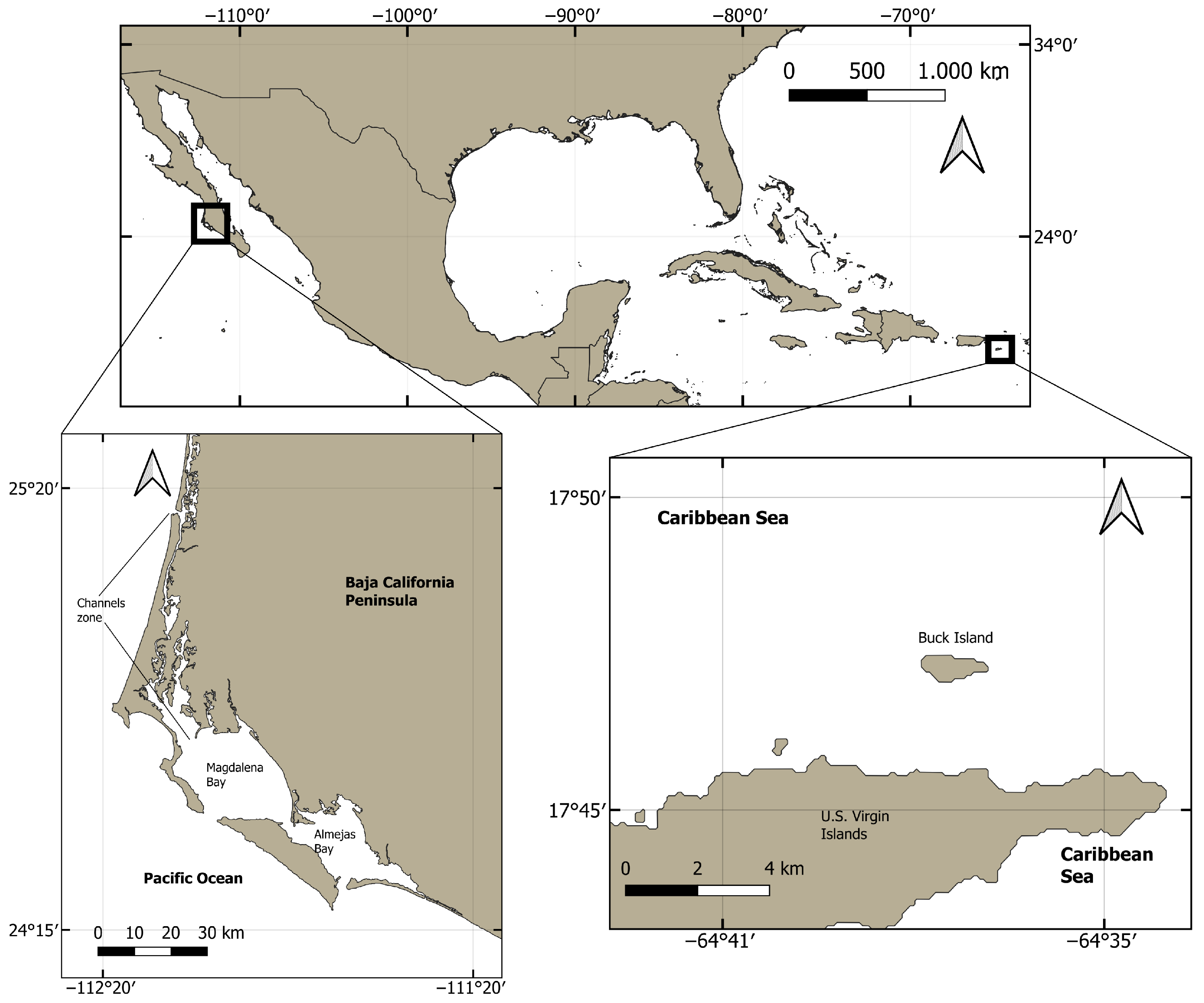
As mentioned in the introduction, two contrasting coastal regions were selected as study areas in order to evaluate the proposed two-stage semiempirical modeling framework. Figure 1 shows the geographic location of both study areas. The left and right panels highlight the study areas.

The first study area is the Magdalena-Almejas Lagoon System, located on the Pacific coast of Baja California Sur, Mexico, between 24°15′–25°20′ N and 111°20′–112°20′ W. This lagoon complex is partially separated from the Pacific Ocean by barrier islands and is one of the largest coastal lagoon systems in the North Pacific. The Magdalena-Almejas system can be divided into three main zones: (i) the northwestern “channels zone,” characterized by a complex morphology of estuaries, lagoons, and tidal channels; (ii) the central zone with Magdalena Bay, which represents the largest portion of the system; and (iii) the southeastern zone with Almejas Bay. Together, these subregions form a heterogeneous environment influenced by tidal exchange, fisheries, aquaculture, and port-related activities. This combination of ecological diversity and anthropogenic use makes it an important area for oceanographic and bathymetric studies. The polygon delimiting this study area is defined by the coordinates listed in

Table 2. Geographic coordinates of the Magdalena-Almejas Lagoon System. The polygon is defined by four corner points corresponding to the upper left (UL), lower left (LL), lower right (LR), and upper right (UR) vertices. Coordinates are expressed in the WGS84 geographic coordinate system.

Point	Description	Latitude (N)	Longitude (W)
1	Upper Left (UL)	25°20′12″	112°19′48″
2	Lower Left (LL)	24°15′12″	112°19′48″
3	Lower Right (LR)	24°15′12″	111°19′48″
4	Upper Right (UR)	25°20′12″	111°19′48″

.

The second study area is the coastal zone surrounding Buck Island, in the U.S. Virgin Islands, located between 17°45′–17°50′ N and 64°41′–64°35′ W. Buck Island and its adjacent waters form part of a protected national monument characterized by clear shallow waters, coral reefs, and high ecological diversity. Unlike the Magdalena-Almejas Lagoon System, this site is an uninhabited island under strong governmental protection, subject to limited anthropogenic influence, and provides a more controlled natural setting. These features make Buck Island particularly suitable for testing satellite-derived bathymetry methods in clear-water conditions. The polygon defining this study area is presented in

Table 3. Geographic coordinates of the Buck Island study area. The polygon is defined by four corner points corresponding to the upper left (UL), lower left (LL), lower right (LR), and upper right (UR) vertices. Coordinates are expressed in the WGS84 geographic coordinate system.

Point	Description	Latitude (N)	Longitude (W)
1	Upper Left (UL)	17°49′44.4″	64°40′48″
2	Lower Left (LL)	17°45′3.60″	64°40′48″
3	Lower Right (LR)	17°45′3.60″	64°34′48′
4	Upper Right (UR)	17°49′44.4″	64°34′48″

.

Although both sites provide valuable testbeds for satellite-derived bathymetry, their benthic environments are markedly different. The Magdalena-Almejas Lagoon System is dominated by sandy sediments and areas of organic matter accumulation, with relatively turbid waters [14]. In contrast, Buck Island features clear waters and a mosaic of habitats, including coral reefs, seagrass meadows, and hard bottoms [1]. These contrasting conditions—one turbid, sediment-dominated lagoon system and one clear-water coral reef environment—are intended to test the robustness and adaptability of the proposed modeling framework.

2.2. Satellite Data and Preprocessing

Landsat 8 Operational Land Imager (OLI) scenes were selected for both study areas due to their 30 m spatial resolution, radiometric quality, and long-term availability. Although Copernicus Sentinel-2 offers higher geometric (10 m) and spectral resolution, Landsat 8 imagery was preferred because of its highly stable radiometric calibration, long temporal continuity, and the availability of the Level-1 Terrain Precision (L1TP) product, which provides systematic corrections using ground control points and digital elevation models. Some authors [15] mention that both images can be effectively used for bathymetry with no alternative being reasonably superior in performance and working with a smaller volume of data in Landsat 8. A total of five images were acquired for the Magdalena-Almejas Lagoon System and two for Buck Island (

Table 4. Dates of Landsat 8 imagery used for the Magdalena-Almejas Lagoon System.

Image ID	Acquisition Date
LC08_L1TP_035043_20180704	4 July 2018
LC08_L1TP_035043_20180805	5 August 2018
LC08_L1TP_035043_20190621	21 June 2019
LC08_L1TP_035043_20211016	16 October 2021
LC08_L1TP_035043_20241109	9 November 2024

and

Table 5. Dates of Landsat 8 imagery used for the coastal zone surrounding Buck Island.

Image ID	Acquisition Date
LC08_L1TP_004048_20190119	19 January 2019
LC08_L1TP_004048_20191119	19 November 2019

). The selection was based on conditions that favor bathymetric retrieval: low turbidity (avoiding periods of high winds or sediment resuspension), less than 5% cloud cover, and tidal levels close to mean sea level (|MSL deviation| < 0.35 m for Magdalena-Almejas, verified with TPXO and tide tables [16]). For Buck Island, a microtidal system, only images from calm meteorological conditions (winds < 5 m/s, based on NOAA data [17]) were considered.

All imagery was obtained from the USGS Earth Explorer platform at the Level-1 Terrain Precision (L1TP) processing level. This dataset provides georeferenced and radiometrically calibrated data, but without atmospheric correction. To retrieve water-leaving reflectance, we applied the ACOLITE algorithm, which is designed for aquatic environments and corrects for atmospheric scattering, absorption, and sun-glint effects. This step ensures reflectance values suitable for shallow-water applications. In addition, reflectance values are converted to floating point numbers by the ACOLITE tool during atmospheric correction, ensuring the appropriate scaling and normalization of Landsat 8 data.

Additional preprocessing steps included cropping each scene to the polygons defining the study areas, reducing computational load, and focusing on the relevant coastal zones. Reflectance values were averaged across dates to reduce radiometric noise and transient variability associated with atmospheric conditions, illumination geometry, and water optical properties. This multitemporal approach enhances the signal-to-noise ratio, mitigates the effects of episodic events, and yields more stable and representative reflectance values for model calibration, thereby improving the robustness and generalization of the bathymetric estimation. In the case of Buck Island, only two images were used because the acquisition dates of the reference dataset were precisely known and the environmental conditions showed very low variability. Conversely, for the Magdalena-Almejas Lagoon System, a larger number of images were averaged due to greater uncertainty in the reference dates and higher temporal variability in water conditions.

Finally, a land mask was generated using the Normalized Difference Water Index (NDWI), calculated from green and near-infrared bands, with a threshold of NDWI > 0 to retain water pixels [18]. This prevented contamination of the bathymetric analysis by land areas.

Images were further screened to exclude “bad-quality” pixels by combining detailed visual inspection with quantitative assessment. We conducted a systematic quality control of the study area subsets derived from the candidate Landsat 8 scenes listed in Table 4 and Table 5 using the QA_PIXEL standard described in the Landsat 8-9 Data Format Control Book [19]. Collection 2 Level-1 QA_PIXEL bitmasks provided by USGS were used to generate cloud masks, excluding pixels flagged as cloudy, shadowed, or affected by cirrus. For each cropped scene, the relative cloud coverage was calculated with respect to valid pixels, yielding consistently low percentages in both study areas (all values below 0.5% for Magdalena-Almejas and below 0.1% for Buck Island). Furthermore, analysis of the QA_PIXEL unique values revealed that more than 93% of valid pixels corresponded to the high-confidence class for open water, indicating negligible contamination from clouds, shadows, snow, or other artifacts. Consequently, only the cropped subsets of these high-quality scenes (those listed in the tables) were retained for further processing, while other candidate acquisitions were discarded for not meeting these criteria.

To further validate the consistency of the retained subsets, spectral variance of the visible bands (red, green, and blue) was computed across valid pixels within each study area. In Magdalena-Almejas, mean variances were on the order of ${10}^{-4}$, while Buck Island presented values of approximately $3\times {10}^{-3}$ across all three bands. These low variances confirm the homogeneity of the cropped images and justify the averaging procedure applied to multiple acquisitions. By reducing residual temporal variability without introducing spurious noise, the averaging of reflectance values enhanced the signal-to-noise ratio and produced stable, high-quality inputs for subsequent bathymetric modeling following the approach in [20]. This preprocessing workflow provided consistent, atmospherically corrected reflectance inputs for both study sites, ensuring comparability between the contrasting environments of a complex Lagoon System and a clear-water protected reef site.

2.3. Proposed Semiempirical Model

The estimation of bathymetry from satellite imagery is traditionally based on the exponential relationship between water depth and spectral reflectance, as described by the Beer–Lambert law. In this formulation, light intensity decreases exponentially with depth due to absorption and scattering, which makes logarithmic transformations a natural choice to linearize the reflectance–depth relationship [2,12]. Semiempirical models, such as those proposed by Lyzenga [3] and Stumpf [4], have successfully exploited this principle. Lyzenga’s method uses log-linear transformations of individual bands, while Stumpf’s widely used approach relies on the ratio of logarithms of two bands. Although both strategies provide transparency and interpretability, they are limited in their capacity to fully capture depth-sensitive spectral variability across diverse coastal environments.

In this work, we propose an alternative formulation based on log-ratio reflectance indices, defined as the logarithm of the ratio between two bands, rather than the ratio of logarithms. This distinction, although subtle, has significant implications: by applying the logarithm directly to the band ratio, the index simultaneously normalizes for illumination effects (as in ratio models) and linearizes the exponential depth dependence (as in log-transform models). This combination seeks to retain the physical interpretability of semiempirical approaches while enhancing stability under different optical conditions.

Two log-ratio reflectance indices are introduced:

$$X_1=log(G/B),X_2=log(R/B)$$

where G, B, and R represent green, blue, and red reflectance values, respectively. The green/blue ratio is sensitive to depth due to the relatively high penetration of green light and reduced absorption compared to other wavelengths, making it particularly suitable for shallow waters. The red/blue ratio, in contrast, captures complementary information from the rapid attenuation of red light, which is valuable for characterizing very shallow zones and enhancing residual contrasts.

To incorporate both indices effectively, we adopt a two-stage regression framework:

• In the first stage, an exponential model is fitted between $X_1$ (green/blue log-ratio) and depth:

  $$Z={\alpha }_1·exp\left({\beta }_1{X}_1\right)+{ϵ}_1$$

  (1)

  where Z is the estimated depth, ${\alpha }_1$ and ${\beta }_1$ are regression parameters, and ${ϵ}_1$ denotes the residuals not explained by the model.
• In the second stage, the residual ${ϵ}_1$ is modeled as a quadratic function of $X_2$ (red/blue log-ratio):

  $${ϵ}_1={\alpha }_2{X}_2^2+{\beta }_2{X}_2+{\gamma }_2$$

  (2)

  where ${\alpha }_2$, ${\beta }_2$, and ${\gamma }_2$ are regression parameters optimized from the data.

Combining both stages yields the final model:

$$Z={\alpha }_1·exp\left({\beta }_1{X}_1\right)+{\alpha }_2{X}_2^2+{\beta }_2{X}_2+{\gamma }_2$$

(3)

This formulation leverages the dominant depth signal from the green/blue index while refining unexplained variance using complementary information from the red/blue index. By structuring the model in two steps, it explicitly accounts for nonlinearities and residual variability, improving predictive accuracy while retaining interpretability.

Model calibration was performed in MATLAB by developing custom functions that used the in situ reference points to minimize the squared error between predicted and observed depths using the Nelder–Mead simplex algorithm (fminsearch).

To benchmark the proposed method, we implemented several semiempirical models from the literature, including those by Lyzenga, Stumpf, and Hashim, as well as a machine learning-based ANN. All the semiempirical models were implemented in MATLAB and calibrated using the same optimization process as in the proposed method, whereas the ANN was trained using MATLAB’s default settings, i.e., one hidden layer of 20 neurons using a tansig transfer function, and a linear output layer (purelin). Training was performed with the Levenberg–Marquardt backpropagation algorithm (trainlm), using 70% of the data for training, 15% for validation, and 15% for testing. The performance function was the mean squared error (MSE), and early stopping was applied if the validation error failed to improve for six consecutive iterations (max_fail = 6). The maximum number of epochs was set to 1000, and the default MATLAB parameters for the Levenberg–Marquardt adjustment (mu initialization and update factors) were used.

Finally, k-fold cross-validation was employed across all models to evaluate generalization capacity and reduce the risk of overfitting, ensuring a fair comparison between approaches. In this procedure, the available dataset is randomly partitioned into k equally sized subsets (folds). At each iteration, one fold is reserved for validation while the remaining $k-1$ folds are used for calibration; the process is repeated k times so that every observation is used for both training and validation exactly once. The final performance metric is obtained by averaging across the k iterations, which provides a robust estimate of model accuracy and stability [21].

2.4. In Situ Data and Validation Strategy

High-quality in situ data are essential for calibrating and validating satellite-derived bathymetry models. In this study, reference measurements served both purposes: part of the dataset was used to estimate model parameters, while the remainder was reserved for independent validation.

For the Buck Island study area, a total of 34,692 points were collected by Leading Edge Geomatics using a Riegl VQ-880-G II sensor, covering depths from 0.01 m to 28.16 m. These airborne LiDAR-derived data, obtained between January and June 2019, provide highly reliable and accurate bathymetric information. Reflectance ranges were red (0.00008–0.3130), green (0.0087–0.3425), and blue (0.0150–0.3321). The abundance and quality of this dataset enable rigorous model testing under clear-water conditions.

According to the accuracy reports included in the metadata, the 2019 NOAA NGS topobathymetric LiDAR survey over Buck Island achieved a horizontal accuracy of ±0.70 m and a bathymetric vertical accuracy of ±0.24 m at the 95% confidence level. These values are well within the requirements of International Hydrographic Organization (IHO) S-44 Order 1a, and the horizontal accuracy even approaches the more stringent thresholds of the Special Order. The reported Non-Vegetated Vertical Accuracy (0.168 m) and Bathymetric RMSE_z (0.236 m) indicate that the dataset provides highly reliable depth measurements suitable for coastal mapping and navigation safety. A comparison between the dataset used and IHO S-44 requirements is presented in

Table 6. Comparison between IHO S-44 accuracy requirements (Special Order and Order 1a) and the reported accuracy of the 2019 NOAA NGS Topobathy LiDAR dataset used for Buck Island.

Criterion	Special Order	Order 1a	LiDAR Dataset
Horizontal accuracy (95% CI)	≤2 m or 2% depth	≤5 m or 5% depth	0.70 m
Vertical accuracy (95% CI)	$\sqrt{0.{25}^2+{\left(0.0075d\right)}^2}$	$\sqrt{0.{50}^2+{\left(0.013d\right)}^2}$	0.24 m
Feature detection	100% coverage, all significant features	Full coverage, detect objects ≥ 2 m	High-resolution LiDAR
Typical application	Harbors, dredging, large vessels	Coastal shallow waters, navigation	Coastal mapping

.

Although the metadata does not explicitly assign a Category Zone of Confidence (CATZOC category), the achieved accuracies are consistent with the standards expected for high-quality hydrographic surveys (CATZOC A2/B) as shown in

Table 7. Summary of LiDAR accuracy metrics as reported in the dataset metadata.

Accuracy Test	Requirement	Reported Value
Horizontal RMSE (95% CI)	≤1.0 m	0.70 m
Non-vegetated Vertical Accuracy (NVA)	0.196 m (95% CI)	0.168 m
Vegetated Vertical Accuracy (VVA)	0.294 m (95th perc.)	0.251 m
Bathymetric RMSEz (95% CI)	0.363 m	0.236 m

. Therefore, this dataset can be considered highly trustworthy for both scientific and operational applications.

For the Magdalena-Almejas Lagoon System, direct measurements were not available, and depths were instead derived from digitized nautical charts. A total of 128 points were extracted, providing coverage across depths from 0.30 m to 25.6 m. Although limited in number, these points represent a valuable reference for assessing the model in a data-scarce context. The corresponding reflectance values for the RGB bands fall within the following intervals: red (0.0043–0.0505), green (0.0133–0.0758), and blue (0.0182–0.0562).

The nautical chart employed for the Magdalena-Almejas Lagoon System corresponds to a historical map published by the U.S. Defense Mapping Agency, based on surveys conducted by the U.S.S. Thetis with subsequent additions and corrections up to 1970. Depths are reported as spot soundings in fathoms, later digitized and converted to metric units for use in this study. Although these data predate the introduction of modern IHO S-44 standards and do not include a formal CATZOC classification, their use is justified by the lack of recent hydrographic surveys in the area, particularly the absence of open-access surveys. The available soundings thus constitute the only reference dataset for calibration and validation of satellite-derived bathymetry in this lagoon system. From a methodological perspective, this provides an opportunity to evaluate the robustness and transferability of the proposed approach under conditions of scarce and uncertain ground-truth data, complementing the high-quality LiDAR-derived dataset available for Buck Island.

Given the spatial resolution of Landsat 8 imagery (30 m), satellite pixels do not coincide exactly with point measurements. To minimize misalignment, the nearest pixel to each geographic coordinate was selected, ensuring the best possible match between reflectance and depth. For each in situ point, we calculate the coordinates of the center of each pixel and assign the in situ point to the pixel whose center is closest. We also verified that no pixel center is assigned to more than one in situ point, avoiding duplication and ensuring that reflectance values are matched consistently to reference depths.

For model development, the data were partitioned into 70% for calibration and 30% for independent validation. Within the calibration set, k-fold cross-validation was applied to optimize model parameters and assess stability. A value of $k=10$ was used for Buck Island, where the dataset is large, and $k=5$ for Magdalena-Almejas, to ensure sufficient data within each fold. This strategy balances robustness with computational feasibility while preventing overfitting.

Model performance was evaluated using four complementary metrics: Root Mean Squared Error (RMSE), Mean Absolute Error (MAE), Coefficient of Determination ($R^2$), and Bias (mean error). RMSE and MAE quantify the overall and average magnitudes of error, respectively; $R^2$ measures the proportion of variance explained; and Bias detects systematic under- or overestimation. In addition, confidence intervals for these indicators were calculated for statistical analysis. Together, these indicators provide a comprehensive assessment of model accuracy and reliability.

Figure 2 shows the distribution of in situ points in both study areas.

3. Results

3.1. Case Study 1: Magdalena-Almejas

Table 8. Performance statistics (mean and std dev) for each benchmark method in the case study 1: Magdalena-Almejas Lagoon System.

Method	${\mathit{R}}^2$	MAE (m)	RMSE (m)	Bias (m)
Lyzenga	0.5506/0.1052	1.3957/0.1005	1.7556/0.0967	−0.4774/0.3008
Stumpf	0.6425/0.0668	1.3372/0.0702	1.6484/0.0523	−0.1682/0.1973
Hashim	0.6178/0.0878	1.3429/0.2114	2.1748/1.3177	0.0236/0.4678
ANN	0.8576/0.0445	0.8585/0.1721	1.1106/0.8431	−0.1207/0.2965
Proposed	0.8155/0.0978	0.9129/0.1545	1.1615/0.7827	0.2836/0.3824

presents the performance comparison between the proposed model and benchmark methods for the Magdalena-Almejas Lagoon System. The reported values correspond to the mean and standard deviation obtained from a 5-fold cross-validation procedure, thus reflecting both the central tendency and the variability of each method’s performance across different partitions of the dataset.

To further estimate the potential robustness of the results, confidence intervals (CI) were computed from the k-fold cross-validation ($k=5$). The standard error was calculated as $\mathrm{SE}=\mathrm{SD}/\sqrt{k}$, and 90% confidence intervals were derived using the t distribution with $df=4$.

For this case study, the proposed method achieved a mean $R^2=0.8155$ (90% CI [0.722, 0.909]), while the best of the semiempirical benchmark strategy, the Stumpf model, yielded $R^2=0.6425$ (90% CI [0.579, 0.706]). The non-overlapping intervals indicate a statistically supported improvement in predictive performance for the proposed approach.

Since the maximum depth in the Magdalena-Almejas case study is $d=25.6$ m, substituting this value into the IHO S-44 expression for the Total Vertical Uncertainty (TVU) at the 95% confidence level yields the following thresholds:

• Special Order: 0.315 m
• Order 1a/1b: 0.601 m
• Order 2: 1.160 m

These values represent the maximum permissible vertical uncertainties defined by IHO S-44 for a depth of 25.6 m, which corresponds to the maximum depth in our study area. Following the IHO recommendation to model vertical uncertainty under a normal distribution and 95% confidence interval. With a mean of 0.9129 m, a standard deviation of 0.1545 m, and $n=38$, the size of the validation data.

The standard error was 0.0251 m and the resulting interval is $0.9129\pm 0.0491$, i.e., $[0.864,0.962]$ m (95% CI, $z=1.96$). Therefore, for this set, an order of 2 in IHO S-44 vertical accuracy would be reached with the proposed method if we had certainty in the in-situ data set. It is important to mention that this category is not achieved with the rest of the semiempirical methods implemented.

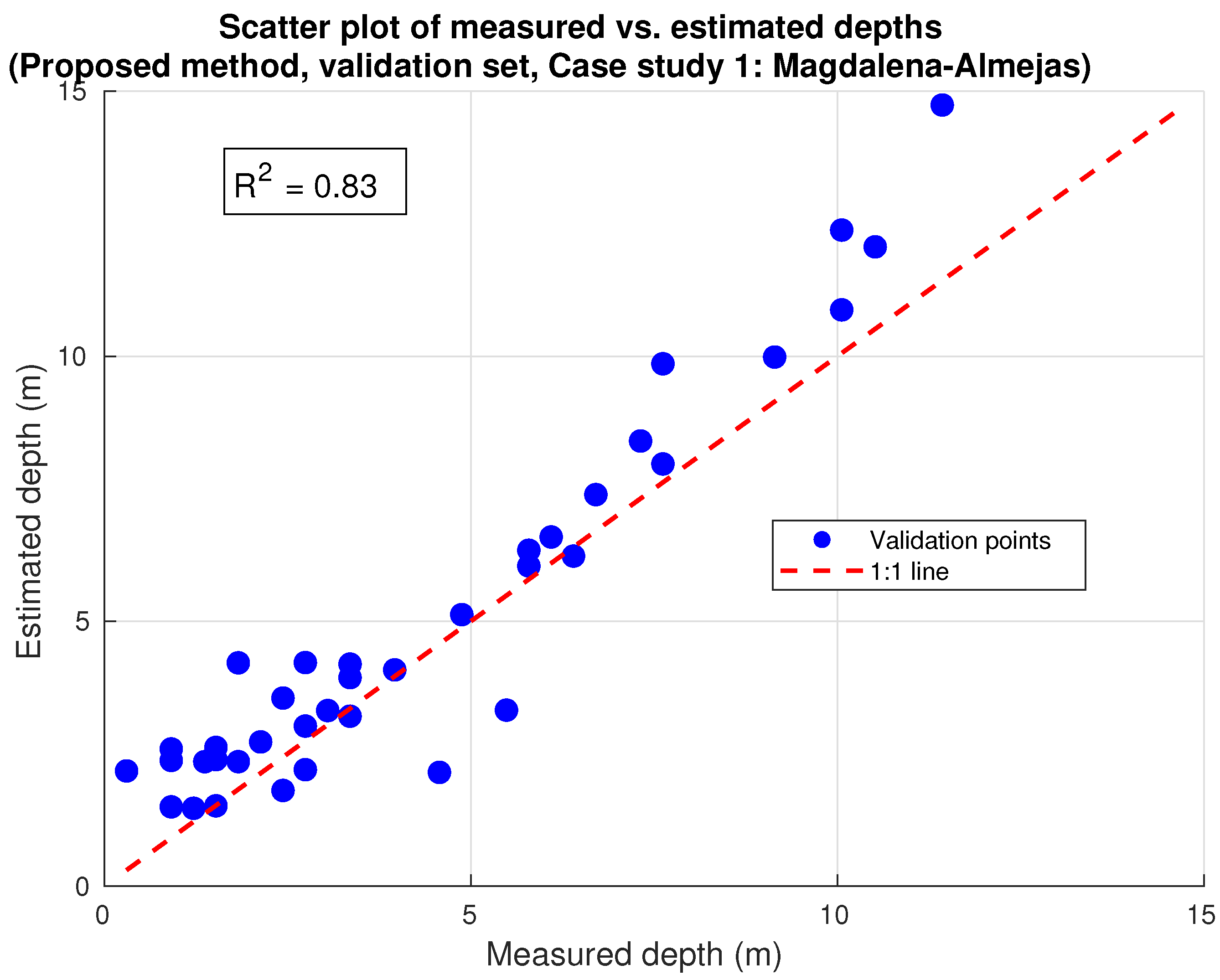
Figure 3 presents the scatter plot of measured versus estimated depths obtained with the proposed method for the validation set in one representative fold of the cross-validation procedure. As previously mentioned, the validation set corresponds to 30% of the data, which in this case comprises 38 points per fold.

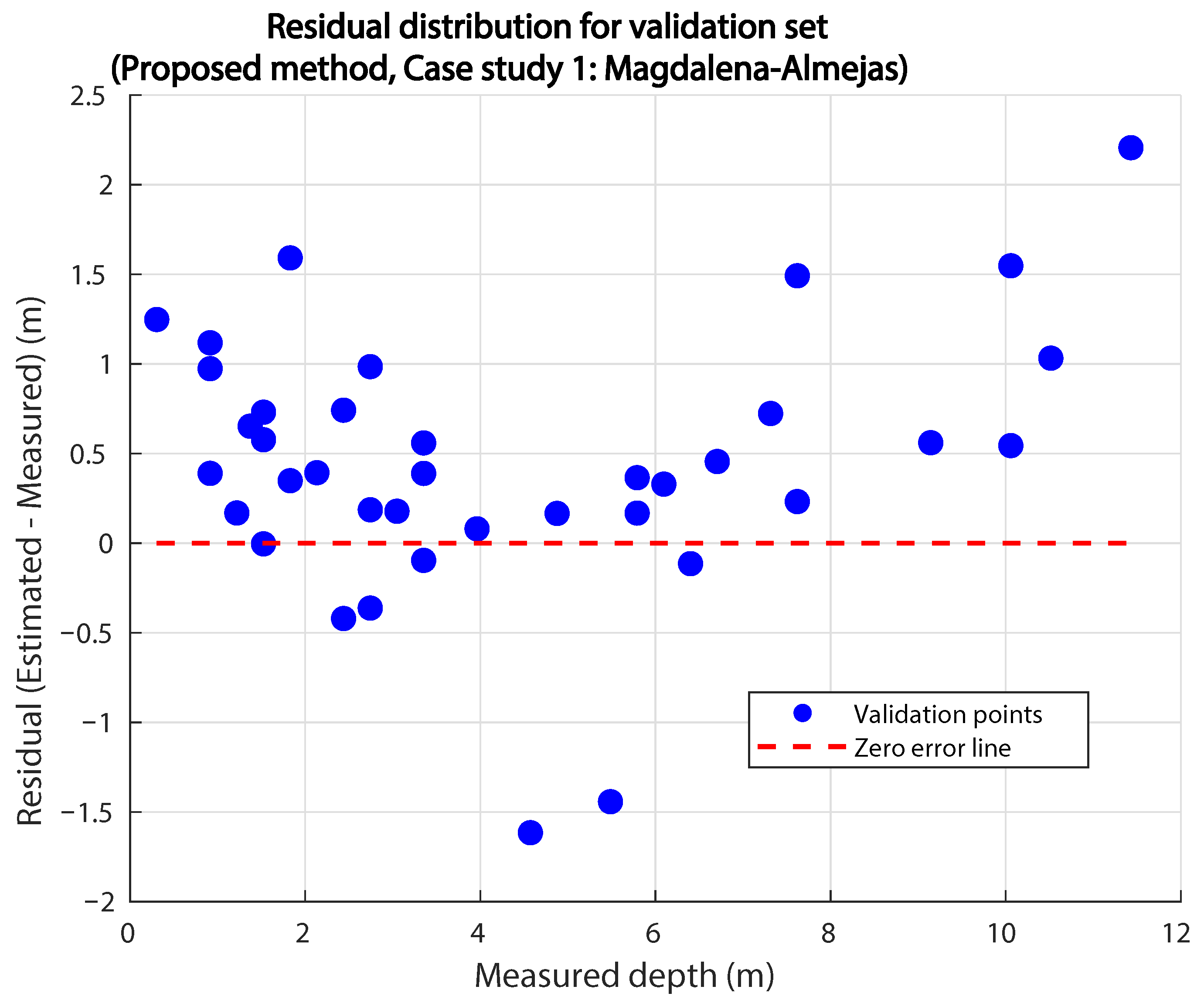
Figure 4 shows the residual distribution, expressed as the difference between the estimated and measured depths, for the validation points in the same fold. This visualization highlights the magnitude and variability of the errors across individual observations.

Finally, Figure 5 illustrates the spatial differences between the bathymetry retrieved with the proposed approach and that obtained using the ANN implementation.

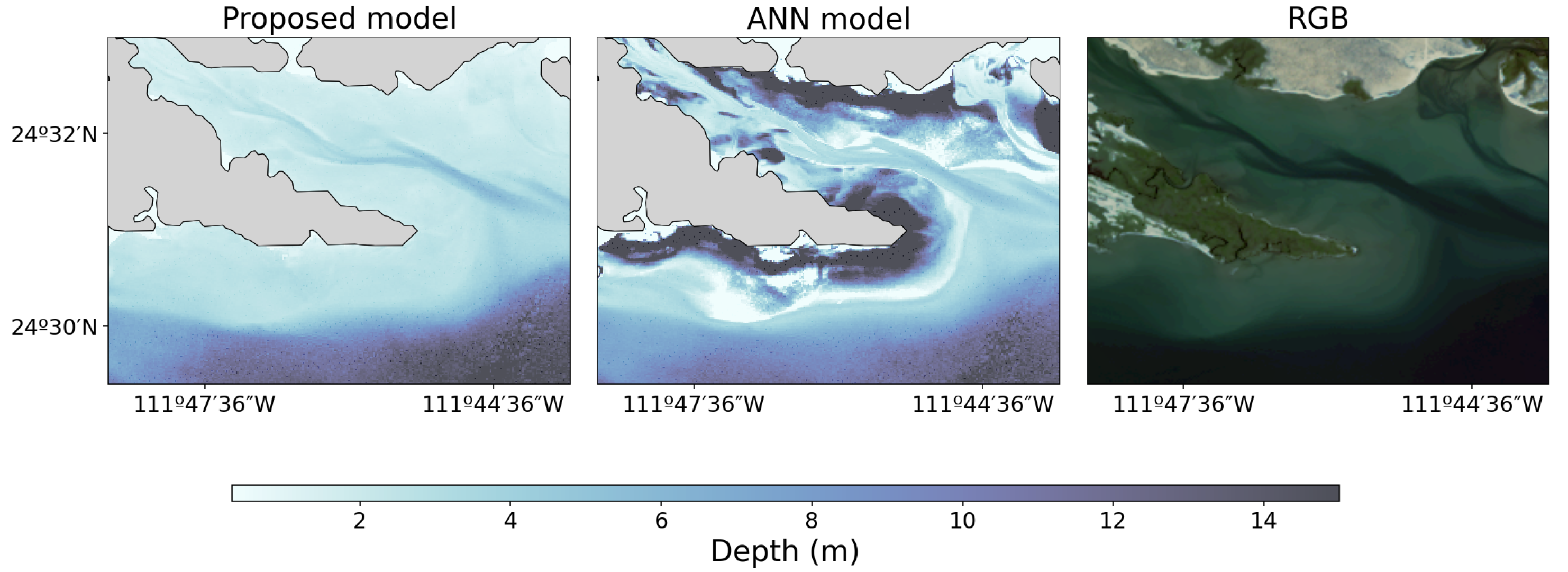
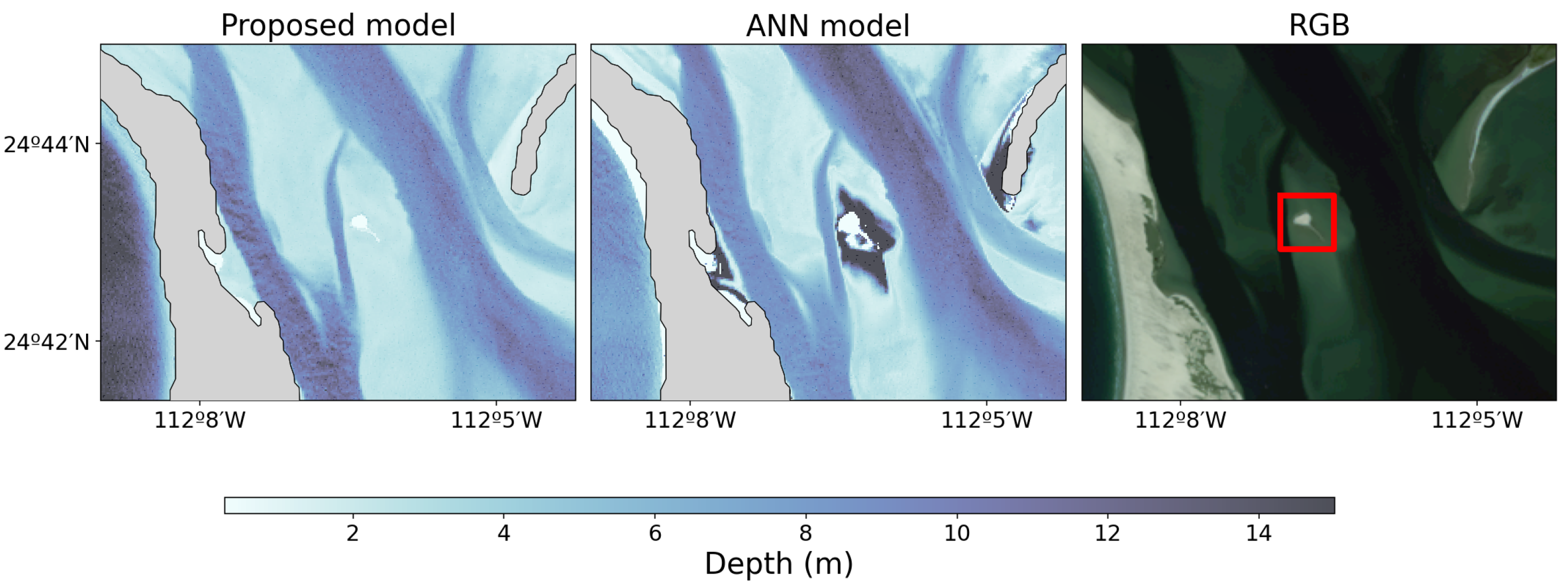
In particular, three regions of interest (A, B, and C) were identified where the ANN exhibited considerable deviations compared to the proposed model, emphasizing the contrasting behavior of both methods in heterogeneous bathymetric settings. Quantitative comparisons were performed wherever in situ reference depth data were available, and these results were presented in the previous section. However, for Regions A, B, and C no ground-truth depth measurements exist, and therefore only qualitative assessments were possible. While such qualitative comparisons are inherently less rigorous, they remain informative by highlighting unrealistic bathymetric artifacts that clearly contradict well-established local knowledge.

• Region A: The ANN produced unrealistic trench-like structures at the tip of Almejas Bay, as shown in Figure 6, where depth is known to be shallow. This is attributed to poor generalization in areas with no training data.
• Region B: The ANN incorrectly extrapolated shallow values surrounding a small island (see Figure 7), overestimating the extent of zero-depth regions (land) and creating non-existent deep areas.
• Region C: A channel-like feature shows an overestimation by the ANN, likely due to extrapolation beyond its training depth range as illustrated in Figure 8. Local actors claim that the depth does not reach 10 m, however the ANN estimates values of up to 14 m.

3.2. Case Study 2: Buck Island

Table 9. For each benchmark method in the case study 2: Buck Island.

Method	${\mathit{R}}^2$	MAE (m)	RMSE (m)	Bias (m)
Lyzenga	0.8872/0.0052	1.0705/0.0071	1.5866/0.0315	0.0041/0.0181
Stumpf	0.8201/0.0029	1.4483/0.0098	2.0097/0.0211	−0.0009/0.0279
Hashim	0.6691/0.0044	2.0875/0.0153	2.7134/0.0275	0.0012/0.0311
ANN	0.9698/0.0010	0.7822/0.0057	1.1391/0.0082	0.0015/0.0143
Proposed	0.9157/0.0016	0.9816/0.0068	1.3769/0.0138	0.0045/0.0165

presents the performance comparison between the proposed model and benchmark methods for Buck Island. The reported values correspond to the mean and standard deviation obtained from a 10-fold cross-validation procedure, thus reflecting both the central tendency and the variability of each method’s performance across different partitions of the dataset.

In this case, confidence intervals were also calculated with standard errors as $\mathrm{SE}=\mathrm{SD}/\sqrt{10}$ and two-sided confidence intervals were derived using the t distribution with $t_{(0.995,9)}=3.250$. The proposed method achieved $R^2=0.9157$ with 99% CI $[0.9141,0.9173]$, whereas the best of the benchmark semiempirical models, Lyzenga model, yielded $R^2=0.8872$ with 99% CI $[0.8819,0.8925]$. The intervals do not overlap even at the 99% confidence level due to the small variance, providing strong statistical support for the superior performance of the proposed approach.

Since the maximum depth in the Buck Island case study is $d=28.16$ m, substituting this value into the IHO S-44 expression for the TVU at the 95% confidence level yields the following thresholds:

• Special Order: 0.341 m;
• Order 1a/1b: 0.698 m;
• Order 2: 1.311 m.

The proposed method achieved a Mean Absolute Error (MAE) of 0.9816 m with a standard deviation of 0.0068 m and $n=10,400$ validation points. The standard error was 0.00007 m and the resulting interval is $0.9816\pm 0.00013$, i.e., $[0.9815,0.9817]$ m (95% CI, $z=1.96$). Therefore, for this set, an Order 2 in IHO S-44 vertical accuracy would be reached with the proposed method.

Figure 9 presents the scatter plot of measured versus estimated depths obtained with the proposed method for the validation set in one representative fold of the cross-validation procedure. As previously mentioned, the validation set corresponds to 30% of the data, which in this case comprises 10,400 points per fold.

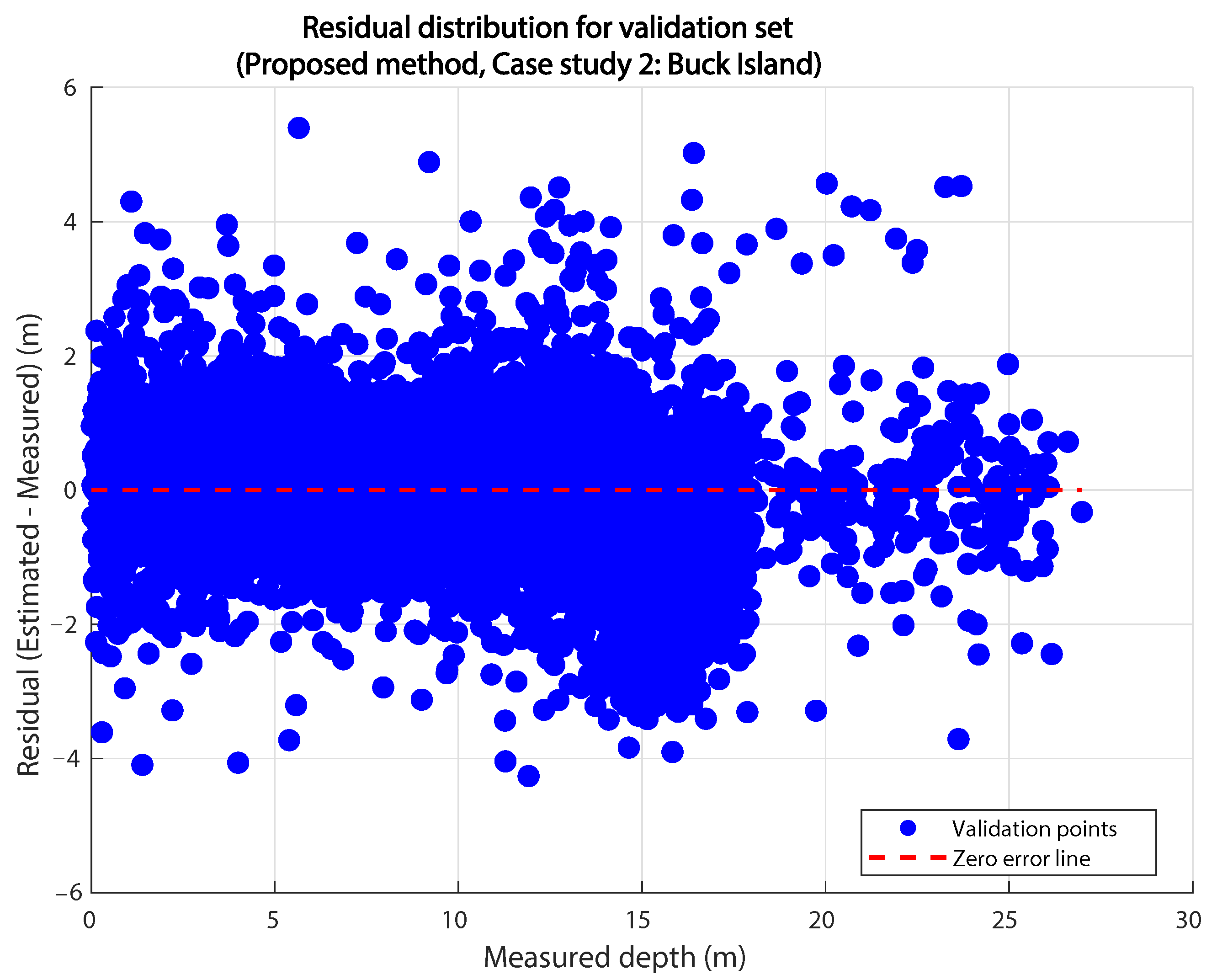
Figure 10 shows the residual distribution, expressed as the difference between estimated and measured depths, for the validation points in the same fold. This visualization highlights the magnitude and variability of the errors across individual observations.

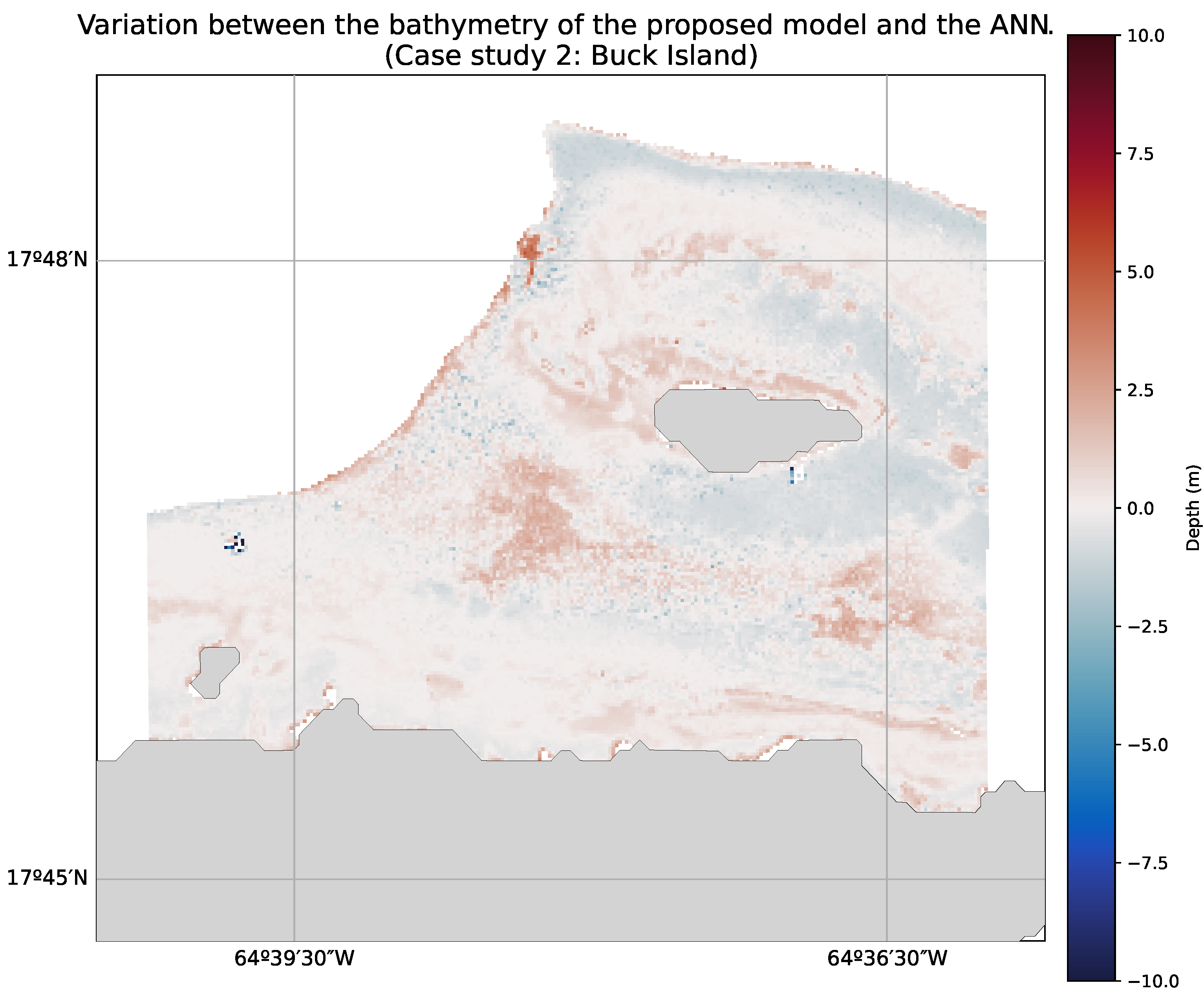
Finally, Figure 11 illustrates the spatial differences between the bathymetry retrieved with the proposed approach and that obtained using the ANN implementation.

In contrast to the Magdalena-Almejas case, the Buck Island results did not reveal localized areas with unrealistically large discrepancies between methods. The dense and high-quality LiDAR dataset ensured that all regions of interest were covered with in situ reference points, preventing the appearance of unvalidated “gaps” where only qualitative assessment would have been possible. As a result, the observed differences between the proposed approach and the ANN remain within the range already quantified through the statistical analysis, with no additional zones requiring separate discussion beyond the quantitative metrics presented above.

4. Discussion

The results from both study areas highlight the advantages and limitations of the proposed two-stage semiempirical model when compared with traditional formulations and machine learning approaches. While artificial neural networks achieved slightly higher numerical accuracy on both test datasets, they showed clear problems in areas lacking training data, such as the heterogeneous regions A, B, and C in the Magdalena-Almejas system. This behavior can be attributed to overfitting and the limited capacity for generalization of ANNs when only sparse or unevenly distributed reference data are available. Given that only 128 chart-derived points were available in this case, it is unlikely that a neural network could capture general patterns robustly, thus reinforcing the advantage of models that embed physical principles.

In contrast, the proposed log-ratio formulation demonstrated spatial consistency across both environments. By combining the optical sensitivity of the green/blue ratio with the attenuation properties of the red/blue ratio, the model captured depth–reflectance relationships more effectively than Lyzenga’s and Stumpf’s formulations in both study areas. Moreover, its interpretability and transparency facilitate reproducibility and environmental decision-making—two aspects that remain problematic with black-box models. The use of log-ratio reflectance indices also proved advantageous for generalization, as they normalize illumination and bottom reflectance variability, conditions especially relevant in turbid and heterogeneous lagoon systems.

The statistical analyses and visualizations further support these findings. Scatter plots showed strong correlations between predicted and measured depths ($R^2$ above 0.81 in turbid waters and above 0.91 in clear-water conditions), while residual distributions did not reveal significant bias: mean errors remained close to zero and both under- and overestimations were balanced across the depth range. This suggests that the model not only reduces the overall error magnitude but also maintains accuracy across different bathymetric zones.

Another important factor relates to preprocessing. The atmospheric correction applied with ACOLITE ensured that reflectance values represented water-leaving radiance by minimizing artifacts from scattering, absorption, and sun-glint. In addition, averaging multiple acquisitions reduced temporal variability due to tides, wind-driven turbidity, and meteorological fluctuations, thereby enhancing the signal-to-noise ratio. Although this smoothing inevitably reduces fine-scale temporal information, it provided stable and consistent spectral inputs for bathymetric retrieval, which likely contributed to the robustness of the proposed approach.

Finally, the nature of the in situ reference datasets must be considered. Buck Island offered highly accurate and dense LiDAR measurements, whereas the Magdalena-Almejas system relied on sparse chart-derived points with uncertain accuracy and unknown CATZOC classification. This comparison illustrates a common operational scenario: LiDAR or multibeam surveys provide reliable ground-truth but are rarely available over extensive areas, while SDB methods are typically applied in precisely those regions where dense or recent datasets are lacking. Acknowledging this limitation is crucial, as the ultimate goal of SDB is not to replicate LiDAR coverage but to provide scalable, cost-efficient estimates where only limited references exist.

In summary, semiempirical models remain more practical in early-stage or resource-constrained studies. Their minimal reliance on large datasets and their physical grounding make them especially suitable for long-term monitoring in developing regions. Nevertheless, in applications where dense and reliable reference data exist, machine learning techniques can complement or surpass semiempirical approaches. Thus, the choice of methodology should be guided by both data availability and operational context.

5. Conclusions

This study proposed and validated a two-stage semiempirical model for satellite-derived bathymetry using log-ratio reflectance indices and Landsat 8 imagery corrected with ACOLITE. The main conclusions are:

• Improved accuracy: The model consistently outperformed traditional semiempirical approaches such as Lyzenga, Stumpf, and Hashim, achieving $R^2=0.8155$ in the Magdalena-Almejas Lagoon System and $R^2=0.9157$ in Buck Island, with RMSE values of 1.16 m and 1.38 m, respectively. Confidence intervals confirmed that these improvements were statistically significant compared to benchmark models.
• Generalization in data-sparse environments: Unlike artificial neural networks, which require large and reliable datasets, the proposed approach maintained robust performance with only 128 chart-derived points in the Magdalena-Almejas case study. This underscores its suitability in contexts with limited or uncertain reference data.
• Interpretability and operational relevance: By leveraging physically meaningful log-ratio reflectance indices, the model preserves transparency and reproducibility. Its adaptability across contrasting environments—turbid lagoon waters and clear coral reef systems—demonstrates its operational value for coastal monitoring and management.
• Role of reference data: The comparison between chart-derived and LiDAR-derived datasets illustrates the dependence of model evaluation on ground-truth quality. While high-resolution LiDAR provides highly accurate validation, SDB methods are most valuable in regions where such dense surveys are not feasible, offering cost-effective and scalable alternatives.

In summary, the proposed log-ratio-based model represents a practical and interpretable strategy for shallow-water bathymetry estimation. While machine learning methods may yield superior accuracy when dense training data are available, semiempirical formulations remain indispensable in operational scenarios where coverage, cost-effectiveness, and interpretability are paramount.

References

1. Caballero, I.; Stumpf, R.P. Towards routine mapping of shallow bathymetry in environments with variable turbidity: Contribution of sentinel-2A/B satellites mission. Remote Sens. 2020, 12, 451. [Google Scholar] [CrossRef]
2. Gülher, E.; Alganci, U. Satellite–Derived Bathymetry in Shallow Waters: Evaluation of Gokturk-1 Satellite and a Novel Approach. Remote Sens. 2023, 15, 5220. [Google Scholar] [CrossRef]
3. Lyzenga, D.R. Shallow-water bathymetry using combined lidar and passive multispectral scanner data. Int. J. Remote. Sens. 1985, 6, 115–125. [Google Scholar] [CrossRef]
4. Stumpf, R.P.; Holderied, K.; Sinclair, M. Determination of water depth with high-resolution satellite imagery over variable bottom types. Limnol. Oceanogr. 2003, 48, 547–556. [Google Scholar] [CrossRef]
5. Hashim, N.S.; Yusof, O.M.; Windupranata, W.; Sulaiman, S.A.H. Integration of Satellite-Derived Bathymetry and Sounding Data in Providing Continuous and Detailed Bathymetric Information. IOP Conf. Ser. Earth Environ. Sci. 2020, 618, 012018. [Google Scholar] [CrossRef]
6. Abr, B.; Ahmed, M.; Marmoush, Y. PlanetScope and Landsat 8 Imageries for Bathymetry Mapping. J. Mar. Sci. Eng. 2020, 8, 143. [Google Scholar] [CrossRef]
7. Caballero, I.; Stumpf, R.P. Confronting turbidity, the major challenge for satellite-derived coastal bathymetry. Sci. Total. Environ. 2023, 870, 161898. [Google Scholar] [CrossRef]
8. Figliomeni, F.G.; Parente, C. Bathymetry from satellite images: A proposal for adapting the band ratio approach to IKONOS data. Appl. Geomat. 2023, 15, 565–581. [Google Scholar] [CrossRef]
9. Mudiyanselage, S.; Abd-Elrahman, A.; Wilkinson, B.; Lecours, V. Satellite-derived bathymetry using machine learning and optimal Sentinel-2 imagery in South-West Florida coastal waters. Giscience Remote Sens. 2022, 59, 1143–1158. [Google Scholar] [CrossRef]
10. Nicolas, K.; Drumetz, L.; Lefèvre, S.; Tiede, D.; Bajjouk, T.; Burnel, J.C. Deep learning–based bathymetry mapping from multispectral satellite data around europa island. In European Spatial Data for Coastal and Marine Remote Sensing: Proceedings of International Conference Eucomare 2022-Saint-Malo 2022, France; Springer: Berlin/Heidelberg, Germany, 2022; pp. 97–111. [Google Scholar]
11. de Andrade, L.C.; Pinheiro, L.P.; Ferreira, Í.O.; das Graças Medeiros, N.; e Silva, A.A. A new approach to satellite-derived bathymetry: The use of NDWI and ANN with bathymetry sections for reservoir mapping. Bull. Geod. Sci. 2024, 30. [Google Scholar] [CrossRef]
12. Hartmann, D.; Gravey, M.; Price, T.D.; Nijland, W.; Jong, S.M.D. Surveying Nearshore Bathymetry Using Multispectral and Hyperspectral Satellite Imagery and Machine Learning. Remote Sens. 2025, 17, 291. [Google Scholar] [CrossRef]
13. Mandlburger, G.; Kölle, M.; Nübel, H.; Soergel, U. Bathynet: A deep neural network for water depth mapping from multispectral aerial images. PFG–J. Photogramm. Remote Sens. Geoinf. Sci. 2021, 89, 71–89. [Google Scholar] [CrossRef]
14. Rodríguez-Meza, D.; Shumilin, E.; Méndez-Rodríguez, L.; Acosta-Vargas, B.; Sapozhnikov, D. Caracterización geoquímica del complejo lagunar Magdalena–Almejas: Sedimentos y macroalgas. In Estudios Ambientales en la región de Bahía Magdalena-Almejas, B.C.S., México; Ulloa, R., Arvizu, J., Eds.; Centro de Investigaciones Biológicas del Noroeste: La Paz, México, 2007; pp. 61–81. Available online: https://www.academia.edu/34561725/Caracterizaci%C3%B3n_geoqu%C3%ADmica_del_complejo_lagunar_Magdalena_Almejas_sedimentos_y_macroalgas (accessed on 8 October 2025).
15. Duan, Z.; Chu, S.; Cheng, L.; Ji, C.; Li, M.; Shen, W. Satellite-derived bathymetry using Landsat-8 and Sentinel-2A images: Assessment of atmospheric correction algorithms and depth derivation models in shallow waters. Opt. Express 2022, 30, 3238–3261. [Google Scholar] [CrossRef] [PubMed]
16. Egbert, G.D.; Erofeeva, S.Y. Efficient inverse modeling of barotropic ocean tides. J. Atmos. Ocean. Technol. 2002, 19, 183–204. [Google Scholar] [CrossRef]
17. National Oceanic and Atmospheric Administration (NOAA). NOAA Tides and Currents Map. 2025. Available online: https://tidesandcurrents.noaa.gov/map/index.html (accessed on 9 June 2025).
18. Laonamsai, J.; Julphunthong, P.; Saprathet, T.; Kimmany, B.; Ganchanasuragit, T.; Chomcheawchan, P.; Tomun, N. Utilizing NDWI, MNDWI, SAVI, WRI, and AWEI for Estimating Erosion and Deposition in Ping River in Thailand. Hydrology 2023, 10, 70. [Google Scholar] [CrossRef]
19. U.S. Geological Survey. Landsat 8–9 Operational Land Imager (OLI)—Thermal Infrared Sensor (TIRS), Collection 2 Level 1 (L1), Data Format Control Book (DFCB). In Data Format Control Book (DFCB); Technical Report Version 7.0; U.S. Department of the Interior: Washington, DC, USA, 2025. [Google Scholar]
20. Wei, C.; Theuerkauf, S. A Novel Multitemporal Approach for Satellite-Derived Bathymetry for Coastal Waters of Palau. J. Coast. Res. 2020, 37, 336–348. [Google Scholar] [CrossRef]
21. Kohavi, R. A Study of Cross-Validation and Bootstrap for Accuracy Estimation and Model Selection. In Proceedings of the 14th International Joint Conference on Artificial Intelligence (IJCAI-95), Montréal, QC, Canada, 20–25 August 1995; Morgan Kaufmann Publishers: San Mateo, CA, USA, 1995; pp. 1137–1143. [Google Scholar]
22. Lamas Torres, F.; Morales Viscaya, J.A.; Tenorio-Fernandez, L. Dataset of In Situ Bathymetric Points and Averaged Reflectance Images for Coastal and Marine Modeling. Zenodo, 2025. Available online: https://doi.org/10.5281/zenodo.15036421 (accessed on 8 October 2025).
Figure 1. Geographic location of the two study areas. Left: Magdalena-Almejas Lagoon System, Baja California Sur, Mexico. Right: Buck Island, U.S. Virgin Islands.
Geomatics 05 00057 g001
Figure 2. Geographic distribution of the dataset points used for bathymetry within the two study areas, the Magdalena-Almejas Lagoon System and the coastal zone surrounding Buck Island.
Geomatics 05 00057 g002
Figure 3. Scatter plot of measured vs. estimated depths with the validation set and using one fold of the proposed method. Case study 1: Magdalena-Almejas.
Geomatics 05 00057 g003
Figure 4. Residual distribution for validation set with the Proposed method, Case study 1: Magdalena-Almejas).
Geomatics 05 00057 g004
Figure 5. Spatial distribution of depth differences between the proposed model and the ANN implementation for the Magdalena-Almejas Lagoon System. Red areas indicate locations where the proposed model predicts greater depths than the ANN, while blue areas denote the opposite case. The map highlights zones with systematic discrepancies between both approaches.
Geomatics 05 00057 g005
Figure 6. Comparison between the bathymetry produced by our proposal, by the ANN, and the RGB image of region A.
Geomatics 05 00057 g006
Figure 7. Comparison between the bathymetry produced by our proposal, by the ANN, and the RGB image of region B.
Geomatics 05 00057 g007
Figure 8. Comparison between the bathymetry produced by our proposal, by the ANN, and the RGB image of region C.
Geomatics 05 00057 g008
Figure 9. Scatter plot of measured vs. estimated depths with the validation set and using one fold of the proposed method. Case study 2: Buck Island.
Geomatics 05 00057 g009
Figure 10. Residual distribution for validation set with the Proposed method, Case study 2: Buck Island.
Geomatics 05 00057 g010
Figure 11. Spatial distribution of depth differences between the proposed model and the ANN implementation for Buck Island. Red areas indicate locations where the proposed model predicts greater depths than the ANN, while blue areas denote the opposite case.
Geomatics 05 00057 g011