Highlights
What are the main findings?
- An end-to-end framework that fuses GIS-derived network features, eXtreme Gradient Boosting (XGBoost), Support Vector Machines, and Dijkstra routing accurately predicts dispatch-to-arrival times and maps fastest fire-response routes for 7421 cleaned incidents in Kayseri.
- XGBoost attains 78.41% accuracy within ±3 min (MAE ≈ 1.67 min, R2 ≈ 0.46), outperforming SVR, while GIS service-area maps reveal that peripheral districts lie beyond the 10-min reach of current stations.
What is the implication of the main finding?
- Fire services gain a real-time, data-driven tool that pairs precise time forecasts with optimal paths, enabling faster, evidence-based deployment and resource reallocation.
- Urban planners and emergency managers can use the scalable GIS-ML workflow to identify coverage gaps, site new stations strategically, and ultimately improve public safety by reducing response delays.
Abstract
This study proposes an integrated, data-driven framework that couples Geographic Information Systems (GIS) with machine-learning techniques to improve fire-department response efficiency in an urban setting. Using an initial archive of 10,421 geocoded fire incident reports collected in Kayseri, Turkey (2018–2023), together with an OpenStreetMap-derived road network, we first generated an “ideal route-time” feature for every incident via Dijkstra shortest-path analysis. After data cleaning and routability checks, 7421 high-quality cases formed the modelling base. Two regression models—eXtreme Gradient Boosting (XGBoost) and Support Vector Regression (SVR)—were trained to predict dispatch-to-arrival times. On the held-out test set, XGBoost yielded the best performance, achieving a mean absolute error of 1.67 min, a root-mean-square error of 2.21 min, a coefficient of determination (R2) of 0.46, and 78.41% accuracy within a ±3 min tolerance. Predicted times were combined with real-time Dijkstra routing to visualize fastest paths and station service areas in GIS, revealing that densely populated districts are reachable within five minutes while peripheral zones exceed ten. The results demonstrate that embedding network-derived features within advanced ML models markedly improves temporal forecasts and that the combined GIS-ML framework can support rapid, evidence-based decision-making, ultimately helping to minimize loss of life and property in urban fire emergencies.
1. Introduction
Fires remain among the most destructive natural and man-made hazards due to their far-reaching ecological and socio-economic consequences. In rapidly urbanizing cities, fire incidents—particularly those occurring near residential areas—pose significant threats to public safety and critical infrastructure. This increasing vulnerability necessitates more effective emergency response strategies and the development of advanced analytical tools to improve intervention times and route efficiency. The time it takes for fire brigades to reach incident locations is a critical determinant of operational success and is influenced by various factors, including the spatial distribution of fire stations, the structure of road networks, real-time traffic conditions, and environmental variables such as weather. As such, reducing response times through predictive modelling and optimized routing has become a central focus of modern emergency management systems.
In recent years, Geographic Information Systems (GIS) and machine learning (ML) techniques have shown great promise in enhancing fire response operations. GIS enables powerful spatial data management and analysis, supporting the identification of risk-prone areas, evaluation of fire station accessibility, and visualization of optimal intervention [1,2]. For instance, GIS-based methods have been employed to assess fire coverage areas [3], estimate travel distances [4], and optimize station locations using multi-criteria decision-making frameworks such as the Analytic Hierarchy Process (AHP) [5,6]. Simultaneously, ML models facilitate the prediction of response times by identifying complex patterns within large-scale datasets. Recent advancements in this domain have seen the application of sophisticated models, such as spatiotemporal graph neural networks (GNN) that incorporate real-time traffic data to achieve higher prediction accuracy [7,8], and deep reinforcement learning approaches for dynamic ambulance dispatching [9]. Models like Support Vector Machines (SVM) and eXtreme Gradient Boosting (XGBoost) remain highly relevant and effective, demonstrating robust performance in various operational contexts, including emergency healthcare and urban mobility systems [10,11,12,13].
While the literature on fire detection using remote sensing technologies, UAV imagery, and computer vision methods is extensive [14,15,16], the critical post-detection phase of operational response has received comparatively less attention. However, many existing GIS-based analyses for emergency response often rely on simplistic models that calculate theoretical travel times based on static distances and speed limits. These approaches frequently overlook complex, real-world factors such as predictable traffic patterns, operational delays, and specific road network configurations that significantly impact actual response times. Consequently, there is a significant gap between theoretically optimal response times and those achieved in practice. Furthermore, while algorithms like Dijkstra’s and its derivatives are widely used for shortest-path analysis in GIS [17,18,19], there remains a notable gap in integrating these algorithms with predictive ML frameworks to enable adaptive, data-informed route planning for fire emergencies, especially when real-time dynamic data is unavailable [20,21,22].
To address this gap, this study proposes and validates a novel, data-driven framework that tightly integrates GIS-based network analysis with advanced ML models to estimate fire department response times in urban settings. The primary novelty of this study lies in its hybrid feature engineering framework, which fundamentally redefines the role of Dijkstra’s algorithm in the predictive pipeline. While many studies use shortest-path algorithms merely as a post-incident operational tool for route identification, our approach proactively utilizes the algorithm’s output. Specifically, the ‘ideal route time’ calculated by Dijkstra is not treated as the final prediction but is instead used as a core predictive feature for the machine learning models. This allows the models to learn the complex, non-linear delta between the theoretical best-case scenario and the operational reality, by analyzing thousands of historical incidents. This integration of a physics-based network model (Dijkstra) with a data-driven learning model (XGBoost/SVR) is the key contribution that enhances predictive accuracy beyond what either method could achieve alone. The study further ensures methodological robustness by excluding records with incomplete network information, thereby focusing on well-connected urban zones where travel-time estimation is reliable.
Through this integration, the study offers both a comparative evaluation of model performance and a demonstration of how GIS-ML synergy can substantially enhance the accuracy and efficiency of fire response operations. Ultimately, the proposed framework represents a scalable, data-driven decision support tool for next-generation urban emergency management systems.
2. Materials and Methods
2.1. General Framework and Workflow
This study implements a six-stage, GIS–ML pipeline to estimate fire department response times and to determine the shortest, time-efficient routes to incident locations (Figure 1). The stages are tightly coupled so that outputs from one feed directly—often programmatically—into the next. The process begins with data collection, where historical fire incidents (2018–2023), OpenStreetMap-based road network layers, and geographic coordinates of active fire stations are compiled for Kayseri. This raw data then undergoes a rigorous cleaning and routability check; records with missing or implausible data are corrected or removed, statistical outliers are filtered, and every incident is tested against the road graph to exclude cases for which no valid path exists. The core of the framework is the hybrid feature engineering stage, where an “ideal route time” is computed for each routable incident using Dijkstra’s algorithm and merged with other temporal and locational attributes. This enriched dataset is then used for response time prediction, training supervised ML models (XGBoost and SVM) and evaluating their performance with metrics like MAE, RMSE, and R2. For operational use, the framework facilitates route optimization by reapplying Dijkstra’s algorithm to identify the fastest path for any new incident. Finally, all outputs are brought together for GIS integration and visualization, creating maps of predicted times, optimal routes, and service-area coverages to support decision-making.
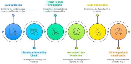
Figure 1.
Workflow diagram of the proposed integrated fire response modelling framework.
2.2. Study Area
Kayseri, the focus of this study, is a major metropolitan city in the Central Anatolia Region of Turkey. Its urban fabric is highly heterogeneous—ranging from dense historic districts to rapidly developing suburban zones—overlaid by an evolving transportation network. These spatial complexities provide an ideal test bed for investigating the key determinants of fire-response performance, including traffic congestion, network accessibility, and the spatial distribution of different fire types.
All fire incident records, fire-station coordinates, and road-network data are confined to the administrative boundaries of Kayseri Province. Figure 2 depicts the geographic dispersion of historical fire events alongside the locations of the five active municipal fire stations. This spatial configuration guided every stage of model development—data preprocessing, network calibration, model training, and validation—ensuring that the analytical results are directly relevant to the operational landscape of the Kayseri Fire Department.
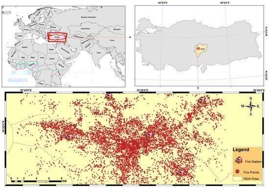
Figure 2.
Spatial distribution of fire incidents and fire station locations in the study area.
2.3. Dataset and Sources
The analytical framework draws on three complementary geospatial datasets—historical fire incident reports, a topologically corrected digital road network, and the coordinates of active fire stations—all integrated within a GIS environment for the Kayseri metropolitan area (Figure 3).
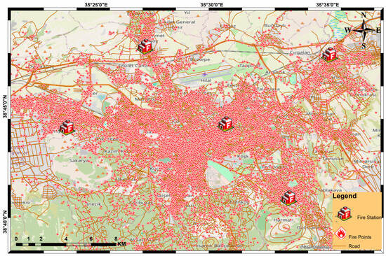
Figure 3.
Detailed spatial distribution of fire incidents (red points), road network (orange lines), and active fire stations (cube icons) across the Kayseri metropolitan area.
2.3.1. Fire Incident Records
The primary dataset, obtained from the Kayseri Metropolitan Municipality Fire Department, comprises a comprehensive archive of 10,421 geocoded fire incident reports spanning five years (2018–2023). Each record contains a rich set of attributes crucial for the analysis, including geographic coordinates (latitude/longitude), the date and time of the incident, the fire category (e.g., structural, vehicle, chimney), the number of responding units, and a full sequence of operational timestamps from dispatch to arrival at the scene. As detailed in the data screening process (Section 2.4), records with data quality issues or non-routable locations were excluded, resulting in a final, analysis-ready subset of 7421 incidents that forms the baseline for modelling. A sample of the attribute data structure is provided in Table 1.

Table 1.
Sample attributes from Kayseri fire incident database.
This enriched incident dataset serves as the foundation for feature engineering and model training described in subsequent sections.
2.3.2. Road Network Data
Reliable traveltime estimation and route optimisation require an up-to-date, topologically consistent road network. Accordingly, the entire street system of the Kayseri metropolitan area was obtained from OpenStreetMap (OSM; OpenStreetMap contributors), a globally recognised opensource platform that is continuously maintained by a community of contributors. The Kayseri road network is characterized by a radial structure originating from the historic city center, transitioning to a more grid-like pattern in newly developed suburban areas. The network consists predominantly of tertiary and residential roads, which influences the overall baseline travel times across the city. The raw OSM layers—comprising carriageways, intersections, and ancillary attributes—were imported into a GIS environment (QGIS) and subjected to a series of preprocessing steps.
First, topological inconsistencies such as dangling edges, overshoots, and duplicate nodes were eliminated to ensure uninterrupted network connectivity. Second, each road segment was enriched with geodesic length and an assumed speed limit based on its OSM road class, allowing travel time weights to be derived as the ratio of length to class-based speed. The specific speeds assigned are detailed in Table 2. Third, the network was converted into a directed graph structure compatible with shortest path algorithms, and its integrity was verified through visual crosschecking against high-resolution satellite imagery and municipal road inventories. The resulting topology corrected digital road network forms the spatial backbone of this study: it underpins both the largescale computation of an “ideal route time” feature for every historical fire incident during preprocessing (Section 2.4) and the real-time application of Dijkstra’s algorithm to identify the fastest path between stations and new incident locations during operational testing.
Table 2.
Assumed Speed Limits for OSM Road Classes.
2.4. Data Preprocessing and Feature Engineering
To ensure the highest possible data quality and model accuracy, all raw inputs—fire incident records, the OpenStreetMap (OSM) road network, and fire station coordinates—were subjected to a four-stage preprocessing pipeline. In the first stage, records with missing or inconsistent values, such as incomplete coordinates or timestamp gaps, were addressed; for instance, missing timestamps were imputed using the median response time for the same district and time of day to preserve the overall data distribution. Extreme outliers in the response time field were identified with a |3|sigma Z score criterion and removed, thereby eliminating anomalous records likely to bias the learning process.
The second stage introduced a hybrid feature engineering step that tightly couples GIS-based network analysis with machine learning. Conventional predictors—such as time of day, day of week, month, and fire category—were retained, but a novel spatial attribute, ideal route time, was computed for every incident. This metric was derived by running Dijkstra’s algorithm on the topologically corrected OSM graph to estimate the fastest travel time between the nearest fire station and the incident location. Routing diagnostics revealed that 3000 incidents were unreachable because of network discontinuities or data quality issues; these records were excluded, leaving a high-integrity modelling subset of 7421 incidents.
A spatial analysis of the excluded incidents revealed a distinct and unexpected pattern (Figure 4). Contrary to the initial hypothesis that data exclusion would primarily occur in peripheral zones due to network sparsity, a high concentration of excluded points was observed within the dense urban core. This finding suggests that data exclusion in this context was likely driven by factors more prevalent in complex urban environments, including: (1) geocoding inaccuracies, where incident addresses were pinned to locations inaccessible by road (e.g., inside building footprints or pedestrian-only zones); (2) micro-level network topology errors in the OSM data, such as incorrectly defined one-way streets or missing connections; and (3) significant data quality inconsistencies in the historical records themselves, such as invalid timestamps that were filtered during preprocessing.
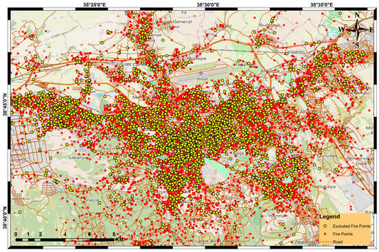
Figure 4.
Spatial Distribution of Included and Excluded Fire Incidents.
During the third stage, the feature matrix was transformed for compatibility with supervised learning algorithms. Categorical variables (e.g., fire type) were one hot encoded, while continuous variables were rescaled: skewed attributes underwent min–max normalisation, and approximately Gaussian variables were standardised with z scores. This scaling uniformity accelerates gradient-based optimisation and mitigates dominance of large magnitude predictors. The final stage entailed a holistic consistency check. Logical constraints—for example, nonnegative dispatch-to-arrival intervals and physically plausible route times—were verified manually and programmatically. The resulting dataset, enriched with both temporal and GIS-derived spatial information, provides a robust foundation for the XGBoost and SVR models described in Section 2.5.
2.5. Fire Response Time Prediction Models
Accurately predicting fire department response times is a core objective of this study. For this purpose, two well-established supervised ML algorithms—Support Vector Regression (SVR) and eXtreme Gradient Boosting (XGBoost)—were implemented, owing to their documented success in emergency response and travel time estimation tasks. Both methods handle nonlinear relationships, scale to high-dimensional data, and offer strong generalization performance. The input features used to train the models are detailed in Table 3.
Table 3.
Predictive features used for response-time modelling.
2.5.1. SVR
SVR, introduced by Vapnik and colleagues, are robust ML algorithms grounded in statistical learning theory. In addition to classification tasks, SVR are widely used for regression problems, known as SVR. The objective of SVR is to construct a function that approximates the relationship between input variables and a continuous target variable within an acceptable error margin ε, while minimizing model complexity. In this study, the Radial Basis Function (RBF) kernel was used to handle non-linear relationships.
A linear SVR model can be expressed as:
where is the weight vector, is the input feature vector, and is the bias term. In the case of non-linear data relationships, input vectors are mapped to a higher-dimensional feature space via a transformation function , leading to:
SVR employs an ε insensitive loss function, which assumes zero error for predictions within the ε threshold and penalizes deviations beyond it. The corresponding optimization problem is formulated as:
subject to:
Here, is the observed response time, is the number of observations, is the regularization parameter balancing model complexity and training error, and are slack variables representing deviations beyond the threshold. The kernel trick is employed for implicit transformation using kernel functions (e.g., linear, polynomial, or radial basis function—RBF), allowing the model to learn complex non-linear patterns effectively.
2.5.2. Extreme Gradient Boosting (XGBoost)
XGBoost, developed by Chen and Guestrin [11], is a high-performance and scalable ensemble learning algorithm based on gradient boosting. It constructs a final prediction by aggregating the outputs of decision trees :
where denotes the space of regression trees. The objective function combines a differentiable loss function and a regularization term :
The loss function for regression is typically Mean Squared Error (MSE), and the regularization term is:
where is the number of leaves in the k-th tree, is the score of the j-th leaf, and γ, λ are regularization parameters. XGBoost employs a second-order Taylor expansion of the objective function and iteratively adds trees that correct the residuals of previous ones, thereby achieving fast training and high accuracy.
2.5.3. Model Training and Evaluation
Both models were trained using fire incident data, where the target variable was the response time from dispatch to on-scene arrival. Independent variables included temporal attributes (e.g., month, day, hour), geographic location, fire type, and other spatio-temporal features derived during the preprocessing phase described in Section 2.4.
The dataset was split into training (80%) and testing (20%) subsets to enable unbiased performance evaluation. After training on the training subset, models were evaluated on the test subset using the following metrics:
Mean Absolute Error (MAE):
Mean Squared Error (MSE):
Root Mean Squared Error (RMSE):
Coefficient of Determination (R2):
where is the mean of the actual response times.
Accuracy within Tolerance Range: Defined as the percentage of predictions falling within a ±3 min threshold, reflecting the model’s practical applicability in emergency scenarios.
These metrics were used to compare the predictive strengths and weaknesses of SVR and XGBoost, ultimately determining the more reliable model for forecasting fire response times.
2.5.4. Hyperparameter Tuning
To maximize model performance, the hyperparameters for both XGBoost and SVR were optimized using a Grid Search methodology coupled with 5-fold cross-validation on the training dataset. This process systematically evaluates a predefined grid of parameter combinations to identify the set that yields the lowest prediction error. The parameter search space and the final optimal values used in the models are summarized in Table 4.
Table 4.
Hyperparameter Tuning Results (5-fold CV, selection metric = MAE).
2.6. Route Optimization Using Dijkstra’s Algorithm
In time-critical emergencies such as urban fires, the ability of response teams to reach an incident location rapidly is a primary determinant of operational success. Consequently, identifying the most time-efficient routes from fire stations to incident sites constitutes a pivotal element of response planning. To solve this shortest-path problem, the well-established Dijkstra algorithm [19] was adopted.
The urban road network—extracted and topologically corrected from OpenStreetMap (Section 2.3.2)—was represented as a directed graph in which nodes correspond to road intersections and edges to road segments. Each edge was assigned a weight reflecting estimated travel time and computed as the ratio of geodesic distance to class-based speed limit.
At runtime, Dijkstra’s algorithm iteratively selects the unvisited node with the smallest tentative distance from the source, relaxes the distances of its neighbours, and marks the node as visited. Formally, the tentative distance of node is updated whenever
where is the current shortest distance to node u. Beginning with = 0 at the source node (fire station) and for all other nodes, the algorithm proceeds until the shortest path to every reachable node is established.
Implemented within the GIS environment, this procedure served a dual purpose. First, it was executed for every historical incident during preprocessing to generate the ideal route-time feature that enriches the machine-learning models (Section 2.4). Second, it was applied in real time to any new or hypothetical incident, yielding a context-aware, fastest path between the optimal station and the incident site. The integration of Dijkstra-derived route times with ML-based arrival-time predictions enabled precise estimation of operational performance under realistic network constraints and provided a robust basis for subsequent spatial visualization and decision support.
2.7. GIS Integration and Visualization
GIS played a central role throughout all stages of this study—from data management and spatial analysis to the integration of modelling results and their effective visualization. The robust geospatial data processing and analytical capabilities of GIS were instrumental in achieving the research objectives and in transforming the results into practically valuable insights.
During the data preparation phase, spatial and attribute datasets such as fire incident records, OpenStreetMap-based road network data, and fire station locations were collected from multiple sources and integrated within the GIS environment. Topological corrections of the road network and its preparation for routing analysis were also conducted using GIS tools [23].
In the route optimization process, the Dijkstra algorithm was implemented using network analysis modules available in GIS. This allowed for the efficient computation of shortest-time routes from fire stations to incident locations, accounting for the complexity of real-world road networks [21]. Furthermore, travel time predictions generated by ML models were spatially linked to corresponding fire events and routes within the GIS environment, enabling a comprehensive spatio-temporal analysis of fire responses.
One of the major outcomes of the study was the spatial visualization and interpretation of these results using GIS. Accessibility zones around fire stations were delineated for multiple travel time thresholds (e.g., 3, 5, and 10 min) through service area (coverage) analysis [24]. Predicted response times and optimized routes were displayed using thematic maps, which revealed the spatial distribution of high-risk fire zones and areas with potential response delays. These maps are particularly valuable for emergency planners in identifying underserved regions and optimizing resource allocation.
For all spatial analyses and mapping tasks, the open-source GIS platform QGIS (version 3.34) was utilized, while MATLAB (R2023a) was employed to support model training and data processing tasks. This hybrid use of GIS and analytical software enabled the construction of a fully integrated decision support framework.
By transforming numerical outputs into geospatially enriched and visually interpretable maps, the proposed GIS-based approach bridges the gap between model outcomes and operational planning [23]. This facilitates actionable insights for decision-makers in areas such as fire response planning, resource allocation, and optimal site selection for future fire stations.
3. Results
This section summarises the outcomes of the integrated GIS-ML analysis carried out for Kayseri. The results focus, first, on a head-to-head comparison of the two response time prediction models—XGBoost and SVR—evaluated with identical test data and error metrics; second, on a feature importance analysis to interpret the model’s drivers; and, third, on the shortest-route analysis performed with Dijkstra’s algorithm, the resulting travel-time outputs, and their integration with the model predictions in a GIS environment to create map-based visualizations of station coverage and optimal intervention routes.
3.1. Model Performance
To train and evaluate the response-time prediction models, we used the final, analysis-ready dataset of 7421 geocoded and routable incidents from the Kayseri Fire Department (2018–2023). The records were randomly partitioned into an 80% training set (5937 cases) and a 20% test set (1484 cases). The split is summarised in Table 5.
Table 5.
Distribution of training and test datasets.
Five evaluation metrics were calculated on the independent test set: Mean Squared Error (MSE), Mean Absolute Error (MAE), Root Mean Squared Error (RMSE), coefficient of determination (R2), and the proportion of predictions falling within a ± 3 min tolerance (Accuracy). Table 6 compares the performance of the optimized XGBoost and SVR models.
Table 6.
Comparative performance of XGBoost and SVR models on the test set.
The results show that the XGBoost model consistently outperforms SVR across all evaluation metrics. With a Mean Absolute Error (MAE) of 1.67 min, the XGBoost model’s predictions are, on average, less than two minutes from the actual arrival time. The model achieved a coefficient of determination (R2) of 0.46, indicating that it can explain approximately 46% of the variance in observed response times—a significant result given the high degree of stochasticity in real-world emergency operations. Operationally, the model accurately predicted 78.41% of response times within the ±3 min tolerance window. Given its superior performance, XGBoost was selected as the primary predictive engine for all subsequent analyses.
To further assess the model’s predictive behavior, visual diagnostic plots were generated for the XGBoost model’s performance on the test set (Figure 5). The scatter plot of predicted versus actual values shows a strong linear relationship, with most points clustered around the ideal 1:1 reference line, confirming the model’s overall accuracy. The residual plot (Figure 6) reveals that the errors are randomly distributed around the zero-error line with no discernible pattern, indicating that the model is not systematically biased. However, a slight increase in variance for longer predicted times (heteroscedasticity) is observable, suggesting that the model’s uncertainty increases for more distant incidents, likely due to unobserved factors such as unexpected traffic or complex routing choices.
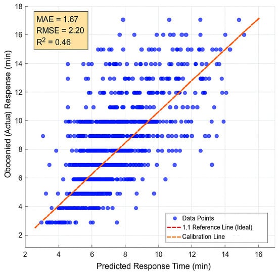
Figure 5.
The scatter plot compares the model’s predicted response times (x-axis) against the actual, observed response times (y-axis) for the 1484 incidents in the test set. Each blue dot represents a single fire event. The dashed red line indicates the 1:1 line of perfect prediction, while the solid orange line shows the regression line of best fit. The clustering of points around the reference line demonstrates the model’s strong predictive performance. Key performance metrics are summarized in the inset box.
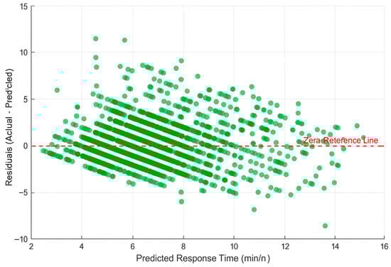
Figure 6.
Residual Plot for the XGBoost Model. The plot shows the residuals (Actual—Predicted response time) on the y-axis against the predicted response times on the x-axis. The random scatter of points around the zero-error reference line (dashed red line) indicates that the model is not systematically biased. A slight increase in the spread of residuals for longer response times suggests mild heteroscedasticity, where the model’s prediction uncertainty grows for more distant or complex incidents.
3.2. Feature Importance Analysis
To enhance the interpretability of the XGBoost model and identify the key drivers of response time, a feature importance analysis was conducted (Figure 7). The analysis utilizes the “gain” metric, which measures the relative contribution of each feature to the model’s predictions. The results reveal that the KNN-derived PastAvgTime (55.2%) and the GIS-derived IdealTime (26.2%) are, by a significant margin, the two most influential predictors. This confirms our central hypothesis: the model’s strength comes from combining a physics-based network baseline (IdealTime) with empirical, learned ‘local knowledge’ (PastAvgTime). This finding reinforces the criticality of providing the model with a physics-based baseline for accuracy. Temporal attributes, particularly Hour of Day and the KNN-derived Past Average Time, also emerged as highly important features, highlighting the impact of predictable traffic patterns and localized, unobserved factors. The incident’s geographic coordinates (Latitude, Longitude) were also significant, demonstrating that the model learns distinct spatial patterns of response delays across the city.
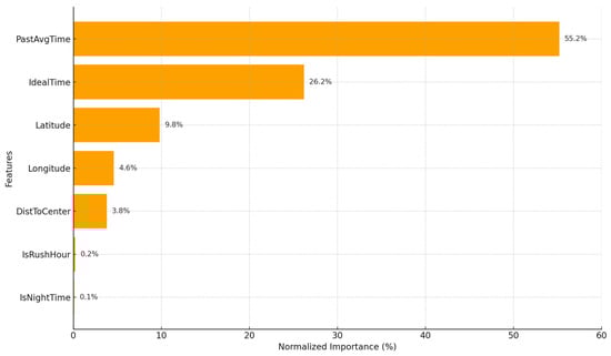
Figure 7.
Feature Importance for the XGBoost Model.
3.3. Shortest Route Analysis and GIS-Based Visualization
The shortest and fastest access routes from each fire station to incident locations were computed with Dijkstra’s algorithm on the routable OSM network described in Section 2.3.2. Figure 8 illustrates a representative case where the value of the integrated framework is demonstrated. For this incident, Dijkstra’s algorithm identified an optimal route with a theoretical ideal route time of 8 min and 5 s. The trained XGBoost model, incorporating learned local factors, predicted a more realistic arrival time of 7 min and 51 s. This prediction, falling very close to the ideal time, represents a scenario where the model successfully confirms a low-congestion route, providing dispatchers with high confidence in the estimate.
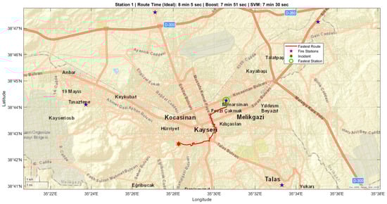
Figure 8.
Visualization of the shortest route to a selected fire incident point over the city map.
The critical value of the ML model, as opposed to relying solely on Dijkstra’s theoretical calculation, is evident when examining specific cases from the test set. For instance, in one incident, the ideal route time calculated by Dijkstra was only 5 min and 16 s. However, the actual recorded response time for this incident was 11 min, a discrepancy of nearly 100%. Our XGBoost model, having learned the patterns of delay associated with that location and time, predicted a response time of 6 min and 56 s. While not perfect, this prediction was significantly closer to the real-world outcome than the theoretical ideal, demonstrating the ML model’s crucial role in bridging the gap between theoretical routing and operational reality. A detailed comparison of ten representative cases from the test set, highlighting a range of scenarios, is provided in Table 7.
Table 7.
Comparison of Ideal, Actual, and Predicted Response Times for Ten Representative Cases.
As illustrated in Table 7, the model’s performance varies across a range of operational scenarios. In cases such as Case 8 and Case 9, the XGBoost model demonstrates high precision, with prediction errors of only about 30 s. These instances represent scenarios where the model’s learned patterns closely align with real-world conditions. Conversely, cases like Case 2 and Case 4, where there is a large discrepancy between the Ideal Time and Actual Time, highlight the most challenging prediction tasks. These significant deviations likely point to unpredictable, real-world events (such as sudden traffic jams, temporary road closures, or on-site operational delays) that are not fully captured by the available features. Overall, the table reinforces that while the model is not infallible, it consistently provides a more nuanced and data-informed estimate than the purely theoretical ‘ideal time,’ effectively acting as a data-driven correction factor to the idealized Dijkstra output.
To evaluate system-wide coverage, a service-area (isochrone) analysis was performed for the five existing stations using the same network graph. Figure 9 maps areas reachable within 3 min (red), 5 min (blue) and 10 min (green).
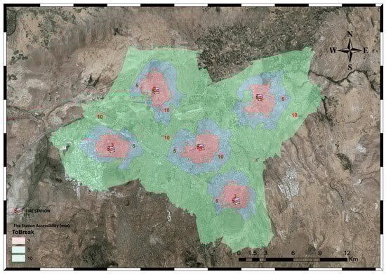
Figure 9.
Fire station accessibility map of Kayseri using service area analysis.
Key observations:
- Central, densely populated districts lie almost entirely inside the 3 to 5 min isochrones, indicating adequate coverage for the majority of incidents.
- Peripheral and semi-rural neighbourhoods often fall outside the 10 min boundary, mirroring response-time disparities reported in previous GIS-based studies [23,24].
- Overlaying the ML-predicted arrival times on these isochrones confirms that the spatial heterogeneity captured by the “ideal route time” feature is reflected in the model outputs, providing a realistic estimation framework.
The combined use of Dijkstra-based routing and XGBoost-based time prediction inside a GIS delivers a holistic, spatially explicit decision-support tool that allows planners to (i) quantify areas of insufficient coverage, (ii) test “what-if” scenarios for new station sites, and (iii) deploy resources along the fastest calculated routes in real time [25].
4. Discussion
This study demonstrates that integrating GIS-based network analysis with machine-learning algorithms can substantially enhance the accuracy of fire-response time prediction and the realism of route planning in urban settings. Using a comprehensive, cleaned dataset of 7421 incidents from Kayseri (2018–2023), the eXtreme Gradient Boosting (XGBoost) model achieved a Mean Absolute Error (MAE) of 1.67 min, a Root Mean Squared Error (RMSE) of 2.21 min, an R2 of 0.46, and 78.41% accuracy within a ±3 min tolerance, clearly outperforming the Support Vector Regression baseline. These results confirm the ability of ensemble tree methods to capture the non-linear, spatio-temporal interactions that govern fire-brigade travel times, echoing the superior learning capacity of XGBoost reported by its originators, Chen and Guestrin [11], and the gains observed in emergency-medical routing studies such as Sheth et al. [26]. The markedly higher R2 relative to traditional linear approaches (e.g., <0.10 in Lian et al. [27]) underscores the value of advanced learners coupled with GIS-driven feature engineering.
A critical aspect of the model’s performance is the interpretation of its evaluation metrics. The low MAE of 1.67 min indicates that the model’s predictions are, on average, very close to the actual arrival times, making it a valuable tool for operational planning. However, the moderate R2 value of 0.46 suggests that while the model effectively captures the systematic and predictable patterns in the data, a significant portion of the variance in response times is driven by factors not included in our feature set. This uncaptured variance likely stems from stochastic (random) real-world events, such as unforeseen traffic accidents, temporary road closures, on-site operational delays at the station, or driver-specific behaviors. Thus, the model excels at predicting the expected arrival time under typical conditions, but the moderate R2 honestly reflects the inherent unpredictability of emergency situations.
The success of the model is largely attributable to the hybrid feature engineering approach. The feature importance analysis revealed that the KNN-derived PastAvgTime and the GIS-derived IdealTime are, by a significant margin, the two most influential predictors. This confirms our central hypothesis: the model’s strength comes from combining a physics-based network baseline (IdealTime) with empirical, learned “local knowledge” (PastAvgTime), which allows the model to learn patterns of predictable traffic congestion and localized, unobserved bottlenecks that are not represented in the static road network data. The overwhelming importance of PastAvgTime suggests that localized, historical performance patterns are the single most powerful predictor of future response times. While this validates the data-driven approach, it also highlights that the model’s accuracy is heavily reliant on the quality and consistency of historical data, and its performance could be sensitive to future systemic changes in traffic infrastructure not reflected in past incidents.
Beyond point predictions, the Dijkstra-based service-area analysis revealed pronounced core-periphery disparities: virtually all central districts are reachable within five minutes, whereas several outlying neighbourhoods fall outside the ten-minute threshold, mirroring spatial inequalities reported in Keratea [23] and Sarajevo [4]. Overlaying the ML predictions on these isochrones provides a unified, map-based picture that emergency managers can exploit to pinpoint underserved zones, test alternative station placements, or adjust shift allocations.
Several limitations merit a more detailed discussion. First, the most significant is the reliance on a static road network and the absence of real-time dynamic data. Real-time traffic congestion and adverse weather conditions (snow, fog, ice) were not directly incorporated, and their inclusion would likely sharpen both the feature inputs and the final estimates. Second, the model’s generalizability is constrained by the characteristics of the dataset. The exclusion of 3000 incidents, which were unexpectedly concentrated in the dense urban core rather than peripheral areas due to data quality issues and routing complexities, highlights a critical limitation. This finding implies that the model’s applicability is contingent not only on the existence of a road network but also on the quality of historical incident data and the topological accuracy of the network representation in complex urban fabrics. Consequently, the model’s performance may be less reliable in central districts with intricate street layouts or where historical data recording practices are inconsistent. Finally, the static speed assumptions used for the Dijkstra calculation, while based on typical limits, were not subjected to a sensitivity analysis to test the model’s robustness to their variation. These factors represent clear avenues for future research. Nevertheless, the proposed workflow—open-source QGIS for network preparation, MATLAB for modelling, and a hybrid GIS–ML feature-engineering loop—offers a reproducible template for other jurisdictions.
In practical terms, the system can be embedded in a dispatch console to recommend the fastest station–route pair and provide a probabilistic arrival window, while the service-area outputs supply planners with an evidence base for long-term resource allocation. By fusing spatial analytics with machine learning, this research highlights the growing role of GIS-centered artificial-intelligence tools in building smarter, more resilient urban emergency-response systems.
5. Conclusions and Recommendations
This study successfully developed and validated a hybrid GIS-ML framework that provides a reliable, data-driven decision-support tool for urban fire services. By integrating Dijkstra’s shortest-path algorithm with advanced machine learning models, the framework moves beyond theoretical routing to predict realistic response times. After a rigorous data cleaning and network integration process on an initial archive of 10,421 incidents, a final dataset of 7421 routable cases from Kayseri (2018–2023) was used for modelling.
The XGBoost model produced the best test-set performance, achieving a Mean Absolute Error (MAE) of 1.67 min, a Root Mean Squared Error (RMSE) of 2.21 min, a coefficient of determination (R2) of 0.46, and 78.41% accuracy within a ±3 min tolerance. The feature importance analysis confirmed that the framework’s predictive power stems from its hybrid feature engineering, which combines a physics-based IdealTime with the learned, empirical “local knowledge” from PastAvgTime. Furthermore, the Dijkstra-based service-area analysis highlighted clear spatial inequities in coverage, with several peripheral districts exceeding the 10 min response threshold. Taken together, this integrated framework provides a powerful tool to help dispatchers choose the fastest station, planners identify underserved zones, and municipal authorities prioritize new facility locations.
Several avenues can further enhance the framework, directly addressing the limitations identified in this study. First, the integration of live data feeds on traffic density, temporary road closures, and adverse weather is the most critical next step to transition the model from a static-historical predictor to a fully dynamic, real-time routing and prediction tool. Second, applying and recalibrating the workflow in cities with different urban morphologies and demand profiles is essential to test its transferability and pave the way for more generalizable, cloud-based platforms. Finally, exploring alternative machine learning architectures, such as LightGBM or spatiotemporal Graph Neural Networks (GNNs), could capture more complex network dependencies and potentially improve predictive accuracy further, while stress-test simulations including road blockages or concurrent disasters would improve robustness.
Embracing such data-driven and AI-supported approaches will be essential for building faster, safer, and more resilient firefighting systems in rapidly urbanising environments.
Author Contributions
T.U.: Conceptualization, Methodology, Software, Validation, Formal analysis, Investigation, Resources, Data curation, Writing—original draft, Writing—review and editing, Visualization, Supervision, Project administration. A.E.: Methodology, Software, Validation, Formal analysis, Investigation, Resources, Data curation, Writing—original draft, Writing—review and editing, Visualization, Supervision. All authors have read and agreed to the published version of the manuscript.
Funding
This research received no external funding.
Institutional Review Board Statement
Not applicable.
Informed Consent Statement
Not applicable.
Data Availability Statement
The original contributions presented in this study are included in the article. Further inquiries can be directed to the corresponding author. The fire incident records used in this study were provided by the Fire Department of Kayseri Metropolitan Municipality and are not publicly available due to data privacy regulations.
Acknowledgments
This study is based on the doctoral dissertation titled “Model Design for Urban Fire Risk Management for Smart Cities”, conducted by Tuğrul URFALI under the supervision of Abdurrahman EYMEN at the Graduate School of Natural and Applied Sciences, Erciyes University. The authors would like to express their gratitude to Erciyes University and the Institute of Science for their support throughout the research process. Special thanks are extended to the Fire Department of Kayseri Metropolitan Municipality for providing access to the fire incident and operational data essential for this research.
Conflicts of Interest
The authors declare no conflicts of interest.
Abbreviations
The following abbreviations are used in this manuscript:
| AHP | Analytic Hierarchy Process |
| CV | Cross-Validation |
| GIS | Geographic Information Systems |
| GNN | Graph Neural Network |
| KNN | K-Nearest Neighbors |
| MAE | Mean Absolute Error |
| ML | Machine Learning |
| MSE | Mean Squared Error |
| OSM | OpenStreetMap |
| RMSE | Root Mean Squared Error |
| SVR | Support Vector Regression |
| SVM | Support Vector Machines |
| UAV | Unmanned Aerial Vehicle |
| XGBoost | eXtreme Gradient Boosting |
References
- Goodchild, M.F. Geographical Information Science. Int. J. Geogr. Inf. Syst. 1992, 6, 31–45. [Google Scholar] [CrossRef]
- Longley, P.A.; Goodchild, M.F.; Maguire, D.J.; Rhind, D.W. Geographical Information Systems. In 1: Principles and Technical Issues; Wiley: New York, NY, USA, 1999; ISBN 978-0-471-33132-2. [Google Scholar]
- Ergezer, F.; Baykal, T.; Terzi, S. Coğrafi Bilgi Sistemleri Kullanılarak Yangın Anında İtfaiye Araçları için Erişilebilirlik Analizi. Isparta İli Örneği. In Proceedings of the 2. Uluslararası Akıllı Ulaşım Sistemleri Konferansı, Bandırma, Turkey, 2–4 May 2024. [Google Scholar]
- SokolovïC, D.; BajrïC, M.; Akay, A.E. Using GIS-Based Network Analysis to Evaluate the Accessible Forest Areas Considering Forest Fires: The Case of Sarajevo. Eur. J. For. Eng. 2022, 8, 93–99. [Google Scholar] [CrossRef]
- Nyimbili, P.H.; Erden, T. GIS-Based Fuzzy Multi-Criteria Approach for Optimal Site Selection of Fire Stations in Istanbul, Turkey. Socioecon. Plann. Sci. 2020, 71, 100860. [Google Scholar] [CrossRef]
- Erden, T.; Coşkun, M.Z. Multi-Criteria Site Selection for Fire Services: The Interaction with Analytic Hierarchy Process and Geographic Information Systems. Nat. Hazards Earth Syst. Sci. 2010, 10, 2127–2134. [Google Scholar] [CrossRef]
- Oluwasanmi, A.; Aftab, M.U.; Qin, Z.; Sarfraz, M.S.; Yu, Y.; Rauf, H.T. Multi-Head Spatiotemporal Attention Graph Convolutional Network for Traffic Prediction. Sensors 2023, 23, 3836. [Google Scholar] [CrossRef]
- Jiang, W.; Luo, J.; He, M.; Gu, W. Graph Neural Network for Traffic Forecasting: The Research Progress. ISPRS Int. J. Geo-Inf. 2023, 12, 100. [Google Scholar] [CrossRef]
- Liu, K.; Li, X.; Zou, C.C.; Huang, H.; Fu, Y. Ambulance Dispatch via Deep Reinforcement Learning. In Proceedings of the 28th International Conference on Advances in Geographic Information Systems, Seattle, WA, USA, 3–6 November 2020. [Google Scholar]
- Cortes, C.; Vapnik, V. Support-Vector Networks. Mach. Learn. 1995, 20, 273–297. [Google Scholar] [CrossRef]
- Chen, T.; Guestrin, C. XGBoost: A Scalable Tree Boosting System. In Proceedings of the 22nd ACM SIGKDD International Conference on Knowledge Discovery and Data Mining, San Francisco, CA, USA, 13 August 2016; ACM: New York, NY, USA, 2016; pp. 785–794. [Google Scholar]
- Yang, A.C.; Ma, W.-M.; Chiang, D.-H.; Liao, Y.-Z.; Lai, H.-Y.; Lin, S.-C.; Liu, M.-C.; Wen, K.-T.; Lin, T.-H.; Tsai, W.-X.; et al. Early Prediction of Sepsis Using an XGBoost Model with Single Time-Point Non-Invasive Vital Signs and Its Correlation with C-Reactive Protein and Procalcitonin: A Multi-Center Study. Intell.-Based Med. 2025, 11, 100242. [Google Scholar] [CrossRef]
- Awan, A.A.; Majid, A.; Riaz, R.; Rizvi, S.S.; Kwon, S.J. A Novel Deep Stacking-Based Ensemble Approach for Short-Term Traffic Speed Prediction. IEEE Access 2024, 12, 15222–15235. [Google Scholar] [CrossRef]
- Yue, W.; Ren, C.; Liang, Y.; Liang, J.; Lin, X.; Yin, A.; Wei, Z. Assessment of Wildfire Susceptibility and Wildfire Threats to Ecological Environment and Urban Development Based on GIS and Multi-Source Data: A Case Study of Guilin, China. Remote Sens. 2023, 15, 2659. [Google Scholar] [CrossRef]
- Özşahïn, E. Cbs ve AHS Kullanılarak Orman Yangını Duyarlılık Analizi: Antakya Orman İşletme Müdürlüğü Örneği. Route Educ. Soc. Sci. J. 2014, 1, 50. [Google Scholar] [CrossRef]
- Tashakkori, H.; Rajabifard, A.; Kalantari, M. A New 3D Indoor/Outdoor Spatial Model for Indoor Emergency Response Facilitation. Build. Environ. 2015, 89, 170–182. [Google Scholar] [CrossRef]
- Wei, H.; Zhang, S.; He, X. Shortest Path Algorithm in Dynamic Restricted Area Based on Unidirectional Road Network Model. Sensors 2020, 21, 203. [Google Scholar] [CrossRef]
- Sahebi, A.; Sayyadi, H.; Havasy, B.; Veisani, Y. Predicting Firefighting Operation Time in Urban Areas Using Machine Learning: Identifying Key Determinants for Improved Emergency Response. Discov. Appl. Sci. 2025, 7, 250. [Google Scholar] [CrossRef]
- Dijkstra, E.W. A Note on Two Problems in Connexion with Graphs. Numer. Math. 1959, 1, 269–271. [Google Scholar] [CrossRef]
- Shmuel, A.; Heifetz, E. A Dijkstra-Based Approach to Fuelbreak Planning. Fire 2023, 6, 295. [Google Scholar] [CrossRef]
- Tian, T.; Wu, H.; Wei, H.; Wu, F.; Xu, M. An Efficient Route Planning Algorithm for Special Vehicles with Large-Scale Road Network Data. ISPRS Int. J. Geo-Inf. 2025, 14, 71. [Google Scholar] [CrossRef]
- Friaswanto, M.; Lisangan, E.A.; Sumarta, S.C. The Simulation of Traffic Signal Preemption Using GPS and Dijkstra Algorithm for Emergency Fire Handling at Makassar City Fire Service. Int. J. Appl. Sci. Smart Technol. 2021, 3, 185–202. [Google Scholar] [CrossRef]
- Yfantidou, A.; Zoka, M.; Stathopoulos, N.; Kokkalidou, M.; Girtsou, S.; Tsoutsos, M.-C.; Hadjimitsis, D.; Kontoes, C. Geoinformatics and Machine Learning for Comprehensive Fire Risk Assessment and Management in Peri-Urban Environments: A Building-Block-Level Approach. Appl. Sci. 2023, 13, 10261. [Google Scholar] [CrossRef]
- Li, J.; Hu, M. Mapping Spatial Inequity in Urban Fire Service Provision: A Moran’s I Analysis of Station Pressure Distribution. ISPRS Int. J. Geo-Inf. 2025, 14, 164. [Google Scholar] [CrossRef]
- Podolskaia, E.; Ershov, D.; Kovganko, K. Spatial Evaluation and Modelling of Fire Stations Layout to Access Forest Fires by Roads (Case Study: Krasecoyarsk Region, Russia). Eur. J. For. Eng. 2024, 10, 112–122. [Google Scholar] [CrossRef]
- Sheth, P.; Patel, P.; Thakkar, P. Optimal Location Prediction for Emergency Stations Using Machine Learning. Int. J. Oper. Res. 2025, 52, 230–251. [Google Scholar] [CrossRef]
- Lian, X.; Melancon, S.; Presta, J.-R.; Reevesman, A.; Spiering, B.; Woodbridge, D. Scalable Real-Time Prediction and Analysis of San Francisco Fire Department Response Times. In Proceedings of the 2019 IEEE SmartWorld, Ubiquitous Intelligence & Computing, Advanced & Trusted Computing, Scalable Computing & Communications, Cloud & Big Data Computing, Internet of People and Smart City Innovation (SmartWorld/SCALCOM/UIC/ATC/CBDCom/IOP/SCI), Leicester, UK, 19–23 August 2019; pp. 694–699. [Google Scholar]
Disclaimer/Publisher’s Note: The statements, opinions and data contained in all publications are solely those of the individual author(s) and contributor(s) and not of MDPI and/or the editor(s). MDPI and/or the editor(s) disclaim responsibility for any injury to people or property resulting from any ideas, methods, instructions or products referred to in the content. |
© 2025 by the authors. Licensee MDPI, Basel, Switzerland. This article is an open access article distributed under the terms and conditions of the Creative Commons Attribution (CC BY) license (https://creativecommons.org/licenses/by/4.0/).