Article

Improving the Temporal Resolution of Land Surface Temperature Using Machine and Deep Learning Models

by
Mohsen Niroomand
1,
Parham Pahlavani
1,
Behnaz Bigdeli
2 and
Omid Ghorbanzadeh
3,*
1
School of Surveying and Geospatial Engineering, College of Engineering, University of Tehran, Tehran 1417935840, Iran
2
Faculty of Civil Engineering, Shahrood University of Technology, Shahrood 3619995161, Iran
3
Institute of Geomatics, University of Natural Resources and Life Sciences, Peter-Jordan Strasse 82, 1190 Vienna, Austria
*
Author to whom correspondence should be addressed.
Geomatics 2025, 5(4), 50; https://doi.org/10.3390/geomatics5040050
Submission received: 6 March 2025 / Revised: 27 March 2025 / Accepted: 27 September 2025 / Published: 1 October 2025

Abstract

Land Surface Temperature (LST) is a critical parameter for analyzing urban heat islands, surface–atmosphere interactions, and environmental management. This study enhances the temporal resolution of LST data by leveraging machine learning and deep learning models. A novel methodology was developed using Landsat 8 thermal data and Sentinel-2 multispectral imagery to predict LST at finer temporal intervals in an urban setting. Although Sentinel-2 lacks a thermal band, its high-resolution multispectral data, when integrated with Landsat 8 thermal observations, provide valuable complementary information for LST estimation. Several models were employed for LST prediction, including Random Forest Regression (RFR), Convolutional Neural Network (CNN), Long Short-Term Memory (LSTM) network, and Gated Recurrent Unit (GRU). Model performance was assessed using the coefficient of determination (R2) and Mean Absolute Error (MAE). The CNN model demonstrated the highest predictive capability, achieving an R2 of 74.81% and an MAE of 1.588 °C. Feature importance analysis highlighted the role of spectral bands, spectral indices, topographic parameters, and land cover data in capturing the dynamic complexity of LST variations and directional patterns. A refined CNN model, trained with the features exhibiting the highest correlation with the reference LST, achieved an improved R2 of 84.48% and an MAE of 1.19 °C. These results underscore the importance of a comprehensive analysis of the factors influencing LST, as well as the need to consider the specific characteristics of the study area. Additionally, a modified TsHARP approach was applied to enhance spatial resolution, though its accuracy remained lower than that of the CNN model. The study was conducted in Tehran, a rapidly urbanizing metropolis facing rising temperatures, heavy traffic congestion, rapid horizontal expansion, and low energy efficiency. The findings contribute to urban environmental management by providing high-temporal-resolution LST data, essential for mitigating urban heat islands and improving climate resilience.

1. Introduction

Land surface temperature (LST) is a vital parameter for understanding the radiative skin temperature of the Earth’s surface [1]. It is primarily influenced by surface emissivity and dynamic energy exchanges between the land and atmosphere [2]. LST plays a crucial role in regulating ecological balance, hydrological cycles, and atmospheric interactions, particularly in both urban and natural environments [3]. It directly impacts vegetation dynamics, the intensity and extent of urban heat islands, and the energy exchange between the terrestrial surface and atmosphere [1,4]. Accurate LST estimation improves climate models, optimizes resource management, and addresses complex environmental challenges [5]. As a key variable, LST enhances our understanding of surface–atmosphere interactions, supporting informed decision making and promoting sustainable management practices [5].
Despite its critical importance, measuring LST presents inherent challenges. Current satellite platforms, such as Landsat, provide LST data with a moderate spatial resolution of 100 m. While suitable for certain applications, this resolution is often insufficient for localized studies, particularly in urban or heterogeneous landscapes [6]. In contrast, higher-resolution sensors like Sentinel-2 lack thermal bands, preventing direct LST measurement. This misalignment between spatial resolution and thermal data availability hinders advancements in urban climatology, agriculture, and ecosystem management [7]. Moreover, the temporal resolution of existing platforms remains inadequate for capturing dynamic LST variations. Landsat’s 16-day revisit interval limits its ability to monitor rapid temperature fluctuations. Although Sentinel-2 offers a 5-day revisit cycle, its lack of thermal sensing creates a critical gap in spatiotemporal LST monitoring [8,9]. Other products, such as ECOSTRESS, provide higher spatial resolution (approximately 70 m) and enhanced temporal frequency, but their limited spatial coverage and inconsistent data availability reduce their suitability for continuous urban monitoring [10]. These limitations in spatial and temporal resolution not only impede scientific progress but also have significant practical implications. Contemporary challenges—such as climate-induced extreme heatwaves, rapid urbanization, and the increasing demand for real-time environmental monitoring—underscore the urgent demand for reliable, high-temporal-resolution LST data [11]. A 5-day revisit capability, combined with advanced data integration methods, supports applications such as urban heatwave early warning systems, real-time agricultural drought assessment, and dynamic energy consumption forecasting in smart cities. Although cloud cover remains a challenge, integrating multi-source data with advanced predictive models helps minimize data gaps, ensuring more continuous and dependable LST monitoring.
The critical importance of high-resolution LST data has highlighted the need to address the temporal and spatial limitations of existing satellite platforms. This growing demand has driven significant advancements in the application of machine learning (ML) and deep learning (DL) techniques. Methods such as artificial neural networks (ANNs), random forests (RFs), and convolutional neural networks (CNNs) offer promising solutions for enhancing the temporal resolution of LST data while improving spatial accuracy beyond the capabilities of traditional algorithms [12,13,14]. These AI-driven approaches refine LST precision and resolution, effectively mitigating gaps in accuracy and spatiotemporal coverage. Such improvements have broad implications in urban climatology, agricultural management, and environmental monitoring [15].
This study aims to address the challenges of predicting high-temporal-resolution LST maps by leveraging advanced machine learning and deep learning models. Beyond utilizing Sentinel-2 spectral bands and Landsat thermal data, the proposed methodology incorporates a comprehensive set of spectral indices, topographic parameters, and land cover classifications as model training features. This integrated approach overcomes limitations arising from varying sensor capabilities and revisit intervals while capturing the complex factors that influence LST. To assess the effectiveness of different techniques, a comparative evaluation of state-of-the-art methods—including RF, long short-term memory (LSTM) network, gated recurrent unit (GRU), and CNN—is conducted. This approach is particularly relevant for rapidly urbanizing environments like Tehran, where heavy traffic, air pollution, and rapid construction significantly impact surface thermal dynamics. The insights derived from this study are expected to contribute to urban climatology research and support the development of effective environmental management strategies.

2. Literature Review

Building upon the significance of LST and its associated challenges, this study reviews relevant literature to highlight recent advancements in improving LST temporal and spatial resolution using machine learning techniques.
Wang et al. (2023) [16] introduced an innovative downscaling approach for ERA5 reanalysis LST products, addressing the challenge of high temporal resolution paired with low spatial resolution. Their method employed a pixel-wise temporal alignment iterative regression model to downscale hourly ERA5 LST data to a spatial resolution of 1000 m. Validation results demonstrated a high coefficient of determination (R2 = 0.87) and a mean absolute error (MAE) of 2.7 K under cloud-free conditions, underscoring the model’s robustness and applicability to all-weather scenarios. Li et al. (2022) [17] utilized Gaofen-6 (GF-6) satellite imagery to downscale LST using remote sensing indices and a random forest-based regression model. Their approach incorporated indices such as the normalized difference vegetation index (NDVI) with red-edge band 2 and the normalized difference sand index (NDSI), enhancing spatial resolution to 16 m and temporal resolution to an 8-day interval. The method achieved high accuracy (R2 = 0.918), providing detailed spatial and temporal insights and meeting the requirements for high-resolution LST analysis. Xu et al. (2021) [14] proposed a multi-factor geographically weighted machine learning (MFGWML) model to downscale LST data from 100 m (Landsat imagery) to 10 m using Sentinel-2 data while improving temporal resolution to 5-day intervals. The model integrated XGBoost, multivariate adaptive regression splines (MARS), and geographically weighted regression (GWR) to enhance predictive accuracy. The approach outperformed traditional methods such as TsHARP and HUTS, with root mean square error (RMSE) values consistently below 2 °C across various regions. Jamaluddin et al. (2021) [18] applied a deep neural network regression (DNNr) approach to estimate LST at a spatial resolution of 10 m and a temporal resolution of 5-day intervals using Sentinel-2-derived NDVI and emissivity data. The model achieved a mean absolute error of 0.58 °C and exhibited a strong correlation with ground-truth data (r = 0.92), highlighting its effectiveness for thermal mapping applications. Ebrahimy and Azadbakht (2019) [13] conducted a comparative study of various machine learning techniques to downscale MODIS LST data from 1 km to 240 m and enhance temporal resolution to an 8-day interval. Their analysis included Random Forest Regression (RFR), Support Vector Regression (SVR), and extreme learning machine (ELM) with a feature selection process. These ML approaches outperformed traditional methods like TsHARP, achieving average performance metrics of RMSE = 2.5 K and MAE = 1.74 K. Notably, the ELM method demonstrated exceptional computational efficiency. Li et al. (2018) [19] applied an RFR model to downscale MODIS LST data from 990 m to 90 m by incorporating multiple predictors, including reflectance bands, spectral indices, terrain factors, and land cover types. The method exhibited high accuracy, with RMSE values of 2.18 K and a coefficient of determination (R2) of 0.9, highlighting the superior performance of RF compared to TsHARP for fine-scale LST applications.
Previous research has explored various indices and methodologies for LST estimation; however, a systematic evaluation of their applicability in urban environments remains limited, particularly regarding the integration of diverse feature sets and the comparative analysis of advanced modeling approaches. Despite recent advancements, comprehensive studies that incorporate various spectral indices, topographic features, and land cover information into LST modeling are still scarce. Moreover, many existing studies focus on a single methodological approach, lacking a systematic comparative assessment of machine learning, deep learning, and traditional models across multi-source data over a well-defined spatial and temporal extent. To address this research gap, the present study integrates 30 distinct features, including spectral bands, spectral indices, topographic data, and land cover data. A comparative analysis is conducted using CNN, LSTM, GRU, and RF models to enhance the temporal resolution of LST estimation in urban settings.

3. Materials and Methods

3.1. Study Area and Dataset

This study utilizes satellite imagery from Landsat 8 and Sentinel-2 to evaluate their effectiveness in estimating LST in Tehran, Iran. Data spanning from July 2019 to 2023 were used for training, while data from July 2024 were reserved for validation. Landsat 8, equipped with the Thermal Infrared Sensor (TIRS), provides essential thermal infrared bands for LST calculation. Meanwhile, Sentinel-2, known for its high-resolution multispectral imagery and 5-day revisit cycle, offers spatial resolutions ranging from 10 to 60 m across various spectral bands, enabling detailed surface analysis. By integrating Landsat 8 thermal data with the spectral richness of Sentinel-2, this study constructed a comprehensive, high-precision dataset that significantly enhances LST modeling accuracy. The selected datasets cover portions of Tehran, a densely populated urban region with complex thermal dynamics. To ensure data quality and reliability, rigorous preprocessing steps—including atmospheric correction and cloud masking—were applied. Figure 1 illustrates the scope of the study area, depicting its geographic location within Iran and providing a detailed spatial representation of Tehran’s administrative boundaries and urban structure.

3.2. Methodology

This study aims to improve the temporal resolution of LST data. LST values derived from Landsat 8 satellite imagery serve as reference labels for model training. The input features include spectral bands from Sentinel-2 satellite images, various spectral indices, topographic data, and land cover classifications. These features are resampled and aligned to match the spatial resolution of the reference data. Several regression algorithms—such as RF, LSTM, GRU, and CNN—are trained on the prepared dataset. The final model is then applied to predict LST in Tehran. The methodology is summarized in Figure 2.

3.2.1. LST Derivation from Landsat Imagery

The precise estimation of LST from Landsat 8 TIRS data necessitates a rigorous methodology that accounts for atmospheric disturbances and surface emissivity variations. The Mono-Window Algorithm (MWA) is a commonly employed technique for deriving LST from Landsat 8 imagery [20]. This method relies on three essential parameters: brightness temperature, land surface emissivity (LSE), and atmospheric properties, including transmittance and the effective mean atmospheric temperature.
Brightness temperature is derived from the digital number (DN) values of band 10, which are first converted to spectral radiance using calibration coefficients provided in the Landsat metadata (MTL) file. The radiance is then transformed into brightness temperature using the inverse Planck function, as shown in Equation (1), where K1 and K2 are constants from the MTL file, and Lλ is the spectral radiance [21].
T 10 = K 2 ln ( K 1 L λ + 1 )
To account for variations in surface properties, land surface emissivity (ελ) is estimated using the NDVI-based approach, which classifies each pixel as vegetation, bare soil, or a mixed surface. This classification is determined based on two threshold values, where NDVIs represents the NDVI of bare soil, and NDVIv corresponds to the NDVI of pure vegetation [21].
For mixed surfaces, where the NDVI falls within the range between NDVIs and NDVIv, the emissivity is computed as a weighted combination of the emissivity values of soil and vegetation. This weighting is determined based on the fractional vegetation cover (Pv), as expressed in Equation (2) [21], where ε and ε represent the emissivities of soil and vegetation, respectively.
ε λ = ε s λ + ( ε v λ ε s λ ) P v
Here, Pv, which quantifies the contributions of soil and vegetation emissivities in mixed pixels, is determined based on NDVI thresholds, as expressed in Equation (3) [21].
P v = N D V I N D V I s N D V I v N D V I s 2
For pixels classified as bare soil (NDVI < NDVIs) or pure vegetation (NDVI > NDVIv), the emissivity is assigned the respective emissivity value corresponding to soil or vegetation, as defined by Equations (4) and (5), respectively [21].
ε λ = ε s λ
ε λ = ε v λ
Atmospheric properties play a fundamental role in ensuring the accuracy of LST estimation. The effective mean atmospheric temperature (Ta) is determined based on near-surface air temperature (T0) through an empirical relationship, as expressed in Equation (6) [21].
T a = 16.011 + 0.9262 T 0
For mid-latitude summer conditions, atmospheric transmittance (τ10) is determined based on water vapor content (w), as expressed in Equation (7) [21].
τ 10 = 0.1134 ω + 1.0335
Once these parameters are determined, LST is calculated using the MWA formula, as presented in Equation (8) [21]:
T s = a 10 ( 1 C 10 D 10 ) + ( b 10 ( 1 C 10 D 10 ) + C 10 + D 10 ) T 10 D 10 T a C 10
where C10 and D10 are defined in Equations (9) and (10), respectively [21].
C 10 = ε λ τ 10
D 10 = ( 1 τ 10 ) [ 1 + ( 1 ε λ ) τ 10 ]
The coefficients a10 and b10 are temperature dependent and are selected accordingly [21]. This approach facilitates precise LST retrieval by accounting for atmospheric corrections and surface emissivity variations, thereby establishing the MWA as a robust method for thermal remote sensing applications.

3.2.2. Data Preparation and Feature Engineering

To ensure data reliability and minimize atmospheric contamination, rigorous cloud-masking procedures were applied. For Landsat 8 imagery, cloud and cloud shadow pixels were identified using the Quality Assessment (QA) band, which provides per-pixel cloud probability metadata [22]. High-confidence cloud and shadow pixels were removed to enhance data quality. For Sentinel-2 imagery, cloud detection was performed using the Sen2Cor atmospheric correction algorithm, which generates a Scene Classification Layer (SCL) to differentiate between clear-sky and cloud-affected pixels [23]. Only clear-sky pixels were retained for feature extraction to ensure robust model training and LST prediction. These preprocessing steps were essential in minimizing atmospheric interference and enhancing the accuracy of high-temporal-resolution LST maps.
The feature set includes several spectral bands from Sentinel-2 satellite imagery, spectral indices derived from these bands, topographic data, and land cover information, all of which are used for training the models. Table 1 summarizes the features utilized in this study.

3.2.3. Model Training

In this study, DL architectures, including CNN, LSTM, and GRU, are employed to predict LST. Their performance is evaluated and compared with the ML method, Random Forest Regression (RFR).
Random Forest Regression (RFR)
RFR is a robust ensemble learning method designed to predict continuous variables by aggregating the predictions of multiple decision trees. This approach mitigates overfitting and enhances generalizability by averaging the predictions from individual trees. The prediction process is mathematically represented in Equation (11) [34]:
y ^ = 1 N i = 1 N T i ( x )
where Ti(x) represents the prediction made by the i-th tree, and N is the total number of trees in the ensemble. In this study, RFR serves as the baseline model, providing a benchmark for evaluating the performance of deep learning approaches. While RFR performs well in low-dimensional contexts, it is limited in modeling complex spatial and temporal patterns [35].
Convolutional Neural Network (CNN)
CNN is a specialized deep learning architecture designed to process spatially structured data. CNN comprises convolutional layers, pooling layers, and fully connected layers, which work together to capture and model spatial dependencies and patterns. This framework makes CNN particularly suitable for predicting LST at high spatial resolutions [36]. The core operation in CNN is the convolution, mathematically expressed in Equation (12) [36]:
y i , j = m = 1 M n = 1 N X i + m , j + n w m , n + b
where yi,j is the output feature map at position (i,j), xi+m,j+n represents the input data, wm,n denotes the kernel weight, and b is the bias term. This operation allows CNN to learn spatial filters that detect edges, textures, and other local patterns in the data. Pooling layers, such as max pooling or average pooling, reduce the spatial dimensions of feature maps while retaining key information. This dimensionality reduction not only alleviates computational demands but also enables the construction of hierarchical feature representations. Fully connected layers at the final stage synthesize these features into task-specific outputs, such as regression predictions or classification probabilities [37].
CNN excels at capturing local spatial relationships and can handle large datasets efficiently due to its parameter-sharing mechanisms. This characteristic significantly reduces computational complexity and memory requirements compared to fully connected networks [38]. Moreover, activation functions like the Rectified Linear Unit (ReLU) introduce non-linearity, improving the model’s ability to capture complex dependencies, as shown in Equation (13) [39].
f ( x ) = max ( 0 , x )
Recent advancements, including batch normalization and dropout, have improved CNN robustness and generalization. Batch normalization standardizes activations during training, addressing internal covariate shift, while dropout helps overfitting by randomly deactivating neurons [40]. A basic CNN architecture is illustrated in Figure 3.
Long Short-Term Memory (LSTM)
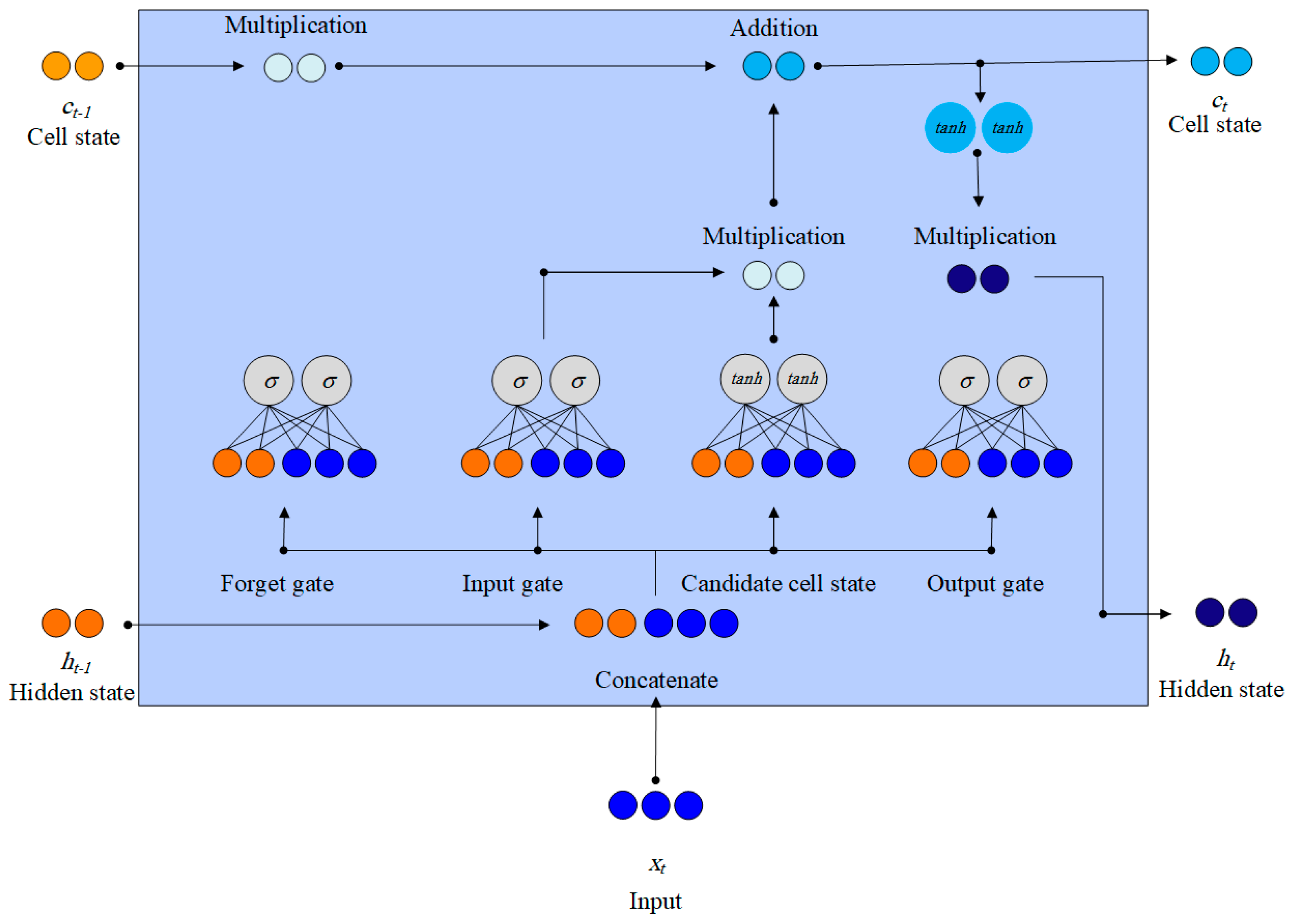
LSTM networks are a specialized form of recurrent neural networks (RNNs) designed to mitigate the vanishing gradient problem and model long-term dependencies within sequential data [41]. An LSTM network achieves this by utilizing a memory cell (ct) along with gating mechanisms—forget gate, input gate, and output gate—that regulate the flow of information within the network [42]. The forget gate determines how much of the previous memory state (ct−1) to retain, as expressed in Equation (14):
f t = σ ( W f . [ h t 1 , x t ] + b f )
where σ is the sigmoid activation function, Wf is the weight matrix for the forget gate, ht−1 is the previous hidden state, xt is the current input, and bf is the bias term for the forget gate [43].
The input gate determines how much new information to incorporate into the cell state, as shown in Equation (15) [43].
i t = σ ( W i . [ h t 1 , x t ] + b i )
The candidate cell state is calculated via Equation (16) [43]:
c ˜ t = tanh ( W c . [ h t 1 , x t ] + b c )
where tanh is the hyperbolic tangent activation function, and Wc and bc are the weight matrix and bias term for the candidate state, respectively. The updated cell state is computed by Equation (17) [43].
c t = f t . c t 1 + i . c ˜ t
Finally, the output gate determines the hidden state ht at time step t as expressed in Equation (18) [43]):
o t = σ ( W o . [ h t 1 , x t ] + b o )
where ot is the output gate, Wo is the weight matrix, and bo is the bias term. The hidden state ht is computed by applying the output gate to the candidate cell state as Equation (19) [43]:
h t = o t . tanh ( c t )
These mechanisms allow LSTM networks to model long-term dependencies, significantly enhancing their performance in time-series analysis and natural language processing tasks. The LSTM architecture is shown in Figure 4.
Gated Recurrent Units (GRUs)
GRUs are a simplified variant of LSTM networks, designed to reduce computational complexity while maintaining strong performance in sequence modeling tasks [44]. Unlike LSTM networks, GRUs combine the forget and input gates into a single update gate (zt), which controls how much past information is retained and how much new information is incorporated. The update gate is calculated using Equation (20) [45]:
z t = σ ( W z . [ h t 1 , x t ] + b z )
where zt controls the update of the hidden state at time step t, and the equation incorporates the previous hidden state ht−1, the current input xt, and their corresponding weight matrix Wz and bias term bz. The sigmoid function σ outputs a value between 0 and 1, determining the extent to which the previous hidden state is retained, and the new information is incorporated into the current state.
The reset gate rt determines how much of the previous hidden state ht−1 should be used in the candidate hidden state h ˜ t , as expressed in Equation (21) [45].
r t = σ ( W r . [ h t 1 , x t ] + b r )
The candidate hidden state is calculated using Equation (22) [45]:
h ˜ t = tanh ( W h . [ h t 1 , x t ] + b h )
where tanh is the activation function, and Wr, Wh, br, and bh are the learned parameters. Finally, the hidden state ht is computed as a weighted combination of the previous hidden state and the candidate hidden state, governed by the update gate, as shown in Equation (23) [45].
h t = z t . h t 1 + ( 1 z t ) . h ˜ t
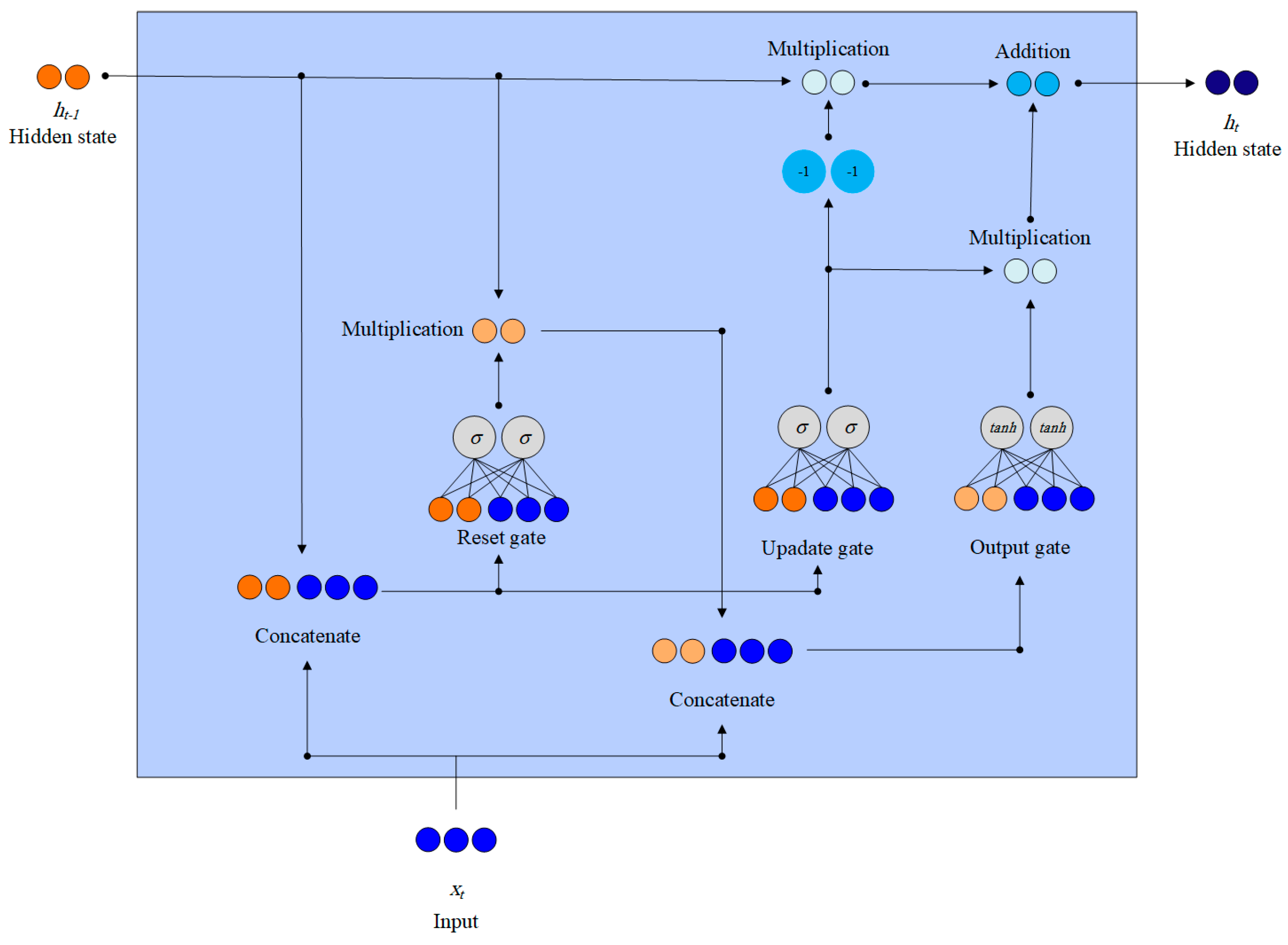
By removing the memory cell and using fewer gating mechanisms, GRUs provide a computationally efficient architecture while delivering performance comparable to LSTM networks for tasks such as time-series prediction and natural language processing [44]. The GRU model architecture is shown in Figure 5.

3.2.4. Model Training Parameters

This section outlines the parameters employed for model training and implementation. For the CNN model, the training dataset consisted of 100,000 independent spatial samples per year from 2019 to 2022. An equivalent number of samples from 2023 were used for validation, and those from 2024 were reserved for testing.
For the GRU and LSTM models, the input data were structured into temporal sequences, with each sample representing the multi-year data of a fixed pixel. The same yearly partitioning was applied for training, validation, and testing.
Hyperparameter tuning was conducted using a grid search approach to identify the optimal configuration for each model. The selection criteria were based on achieving the lowest mean squared error (MSE) and the highest R2 on the validation set. The tested hyperparameters ranges for each model are summarized in Table 2.
The RFR model was employed to predict LST, with its optimal configuration—250 estimators, a maximum depth of 30, and a minimum samples split of 5—determined via grid search [46]. Leveraging its ensemble learning framework, RFR demonstrated robust predictive performance and effectively handled high-dimensional input features.
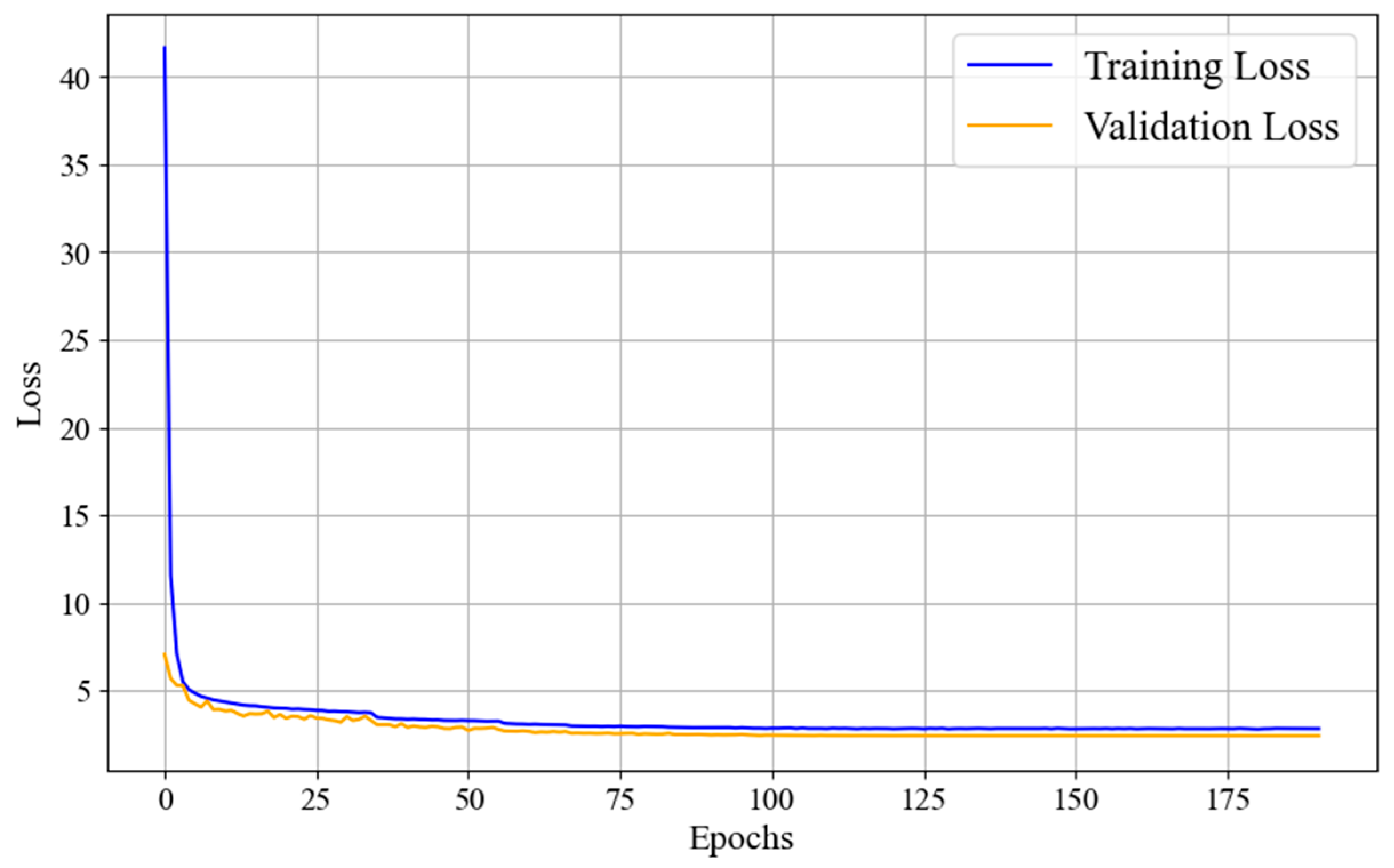
To further enhance LST prediction, advanced deep learning architectures were implemented. The CNN model consisted of three convolutional layers with 256, 128, and 64 filters, each followed by ReLU activation functions [47]. A dropout layer with a rate of 0.3 was applied after the convolutional layers to mitigate overfitting. The extracted feature maps were flattened and passed through three fully connected layers with 128, 64, and 32 units before reaching the final output layer, which consisted of a single neuron with a linear activation function [48]. The CNN model was initially trained using a grid search to select learning rates of 10−3, 10−4, and 10−5, with 10−5 yielding the best validation performance. To further refine convergence, an adaptive learning rate strategy was applied, ultimately adjusting the learning rate to 3.9063 × 10⁻⁶ through fine-tuning. Training was conducted for up to 500 epochs with a batch size of 16, incorporating early stopping (halting training at epoch 109) and learning rate reduction callbacks.
Additionally, LSTM and GRU networks were explored. Both architectures followed a sequential configuration with four layers containing 256, 128, 64, and 32 units, each activated by ReLU functions. The output from the final layer was passed through two dense layers with 32 and 16 units before reaching the final output layer. These models were trained using the Adam optimizer [49], with an initial learning rate of 10−3 and MSE as the loss function. Training was performed for up to 500 epochs with a batch size of 16, incorporating early stopping and learning rate reduction strategies. The LSTM model halted at epoch 146, while the GRU model converged at epoch 171. In both cases, the learning rate was reduced to 10−6 upon observing a plateau in performance metrics.
For all neural network models, MSE was used as the loss function, as it is well-suited for continuous regression tasks like LST estimation. MSE penalizes larger errors more heavily than smaller ones, making it effective for minimizing deviations between predicted and observed LST values.

3.2.5. Feature Importance Analysis

To better understand the contributions of individual predictors in LST estimation, feature importance analysis was performed using SHAP (SHapley Additive exPlanation) values. The SHAP framework assigns an importance score to each feature by quantifying its effect on the model output. The SHAP value for a given feature i is defined as Equation (24) [50]:
ϕ i = S N \ { i } S ! ( N S 1 ) ! N ! [ f ( S { i } ) f ( S ) ]
where S denotes a subset of all features N that does not include feature i, and f(S) represents the model output when only the features in S are present. A heat map is generated to visualize the mean absolute SHAP values for each feature, providing a clear and interpretable representation of their relative importance.

3.2.6. Sharpening Thermal Imagery

The Sharpening Thermal Imagery (TsHARP) method, a widely used thermal downscaling technique, was applied to enhance the spatial resolution of LST data in urban areas. The traditional TsHARP approach establishes a relationship between LST and NDVI; however, in urban environments, LST correlates more strongly with impervious surfaces. Therefore, the Normalized Difference Built-up Index (NDBI) was used as an alternative to NDVI. The impervious surface fraction (FIS) was calculated using Equation (25) [51]:
F I S = N D B I N D B I m i n N D B I max N D B I m i n
where NDBImin and NDBImax represent the minimum and maximum NDBI values in the study area, respectively. A linear regression was then established between the upscaled impervious surface fractions (FISC) and LST at a coarse resolution, as shown in Equation (26) [51].
T C = a 0 + a 1 × F I S C
The regression parameters a0 and a1 were then applied to the high-resolution impervious surface fraction map (FISF) to generate the downscaled LST map using Equation (27) [51].
T F = a 0 + a 1 × F I S F
Finally, the residual difference between the coarse-scale LST and the regression-derived LST was computed and bilinearly resampled to refine the final downscaled LST product. This modified TsHARP approach provides an effective alternative method for improving LST resolution in urban settings.

3.2.7. Evaluation Metrics

A rigorous assessment of model performance and feature relevance was conducted using statistical evaluation metrics. Pearson’s correlation coefficient was computed to quantify the linear relationship between each predictor variable and the observed LST. This coefficient, ranging from –1 to 1, indicates both the strength and direction of the association [52]. Values close to ±1 signify strong correlations, whereas values near 0 suggest weak or negligible linear relationships. This analysis helped identify the most influential predictors for LST estimation.
To further evaluate predictive accuracy, two statistical measures were employed. The first metric, the coefficient of determination (R2), quantifies the proportion of variance in the observed LST values that is explained by the model [53]. Higher R2 values indicate better model performance, signifying a stronger agreement between predicted and observed values. The R2 value is calculated as shown in Equation (28) [53]:
R 2 = 1 i = 1 n ( y i y ^ i ) 2 i = 1 n ( y i y ¯ ) 2
where yi and y ~ i represent the observed and predicted values, respectively, y ¯ is the mean of the observed values, and n is the number of data points.
The second metric, the Mean Absolute Error (MAE), measures the average discrepancy between predicted and observed LST values, expressed in degrees Celsius. It provides a straightforward representation of the magnitude of prediction errors. Lower MAE values indicate greater model precision and reliability in LST estimation. The MAE is calculated as shown in Equation (29) [54].
M A E = 1 n i = 1 n y i y ^ i

4. Results

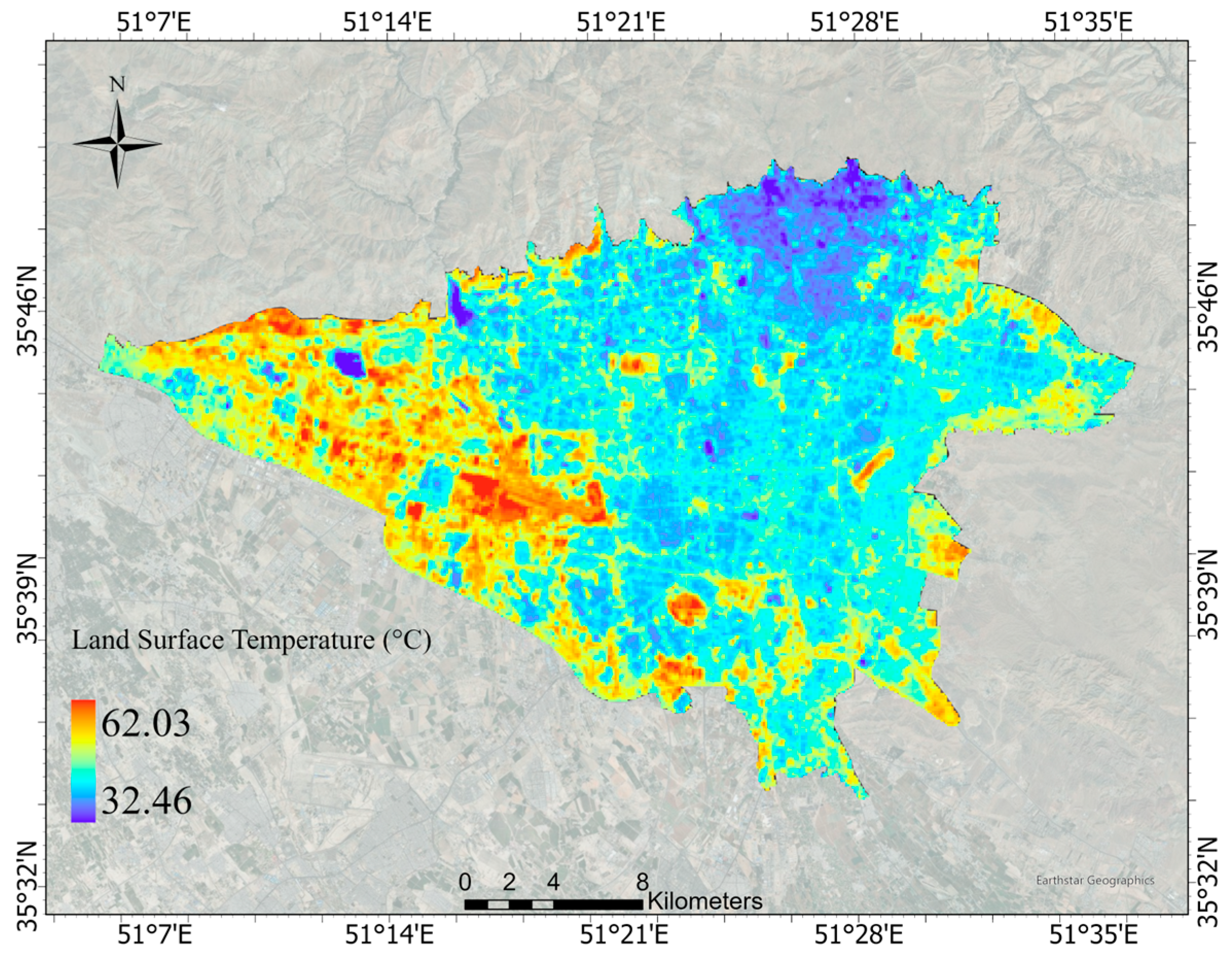
The reference LST values were derived from Landsat 8 imagery acquired annually from July 2019 to 2024, with 100,000 samples selected each year for analysis. Figure 6 illustrates the LST values for Tehran in July 2024.
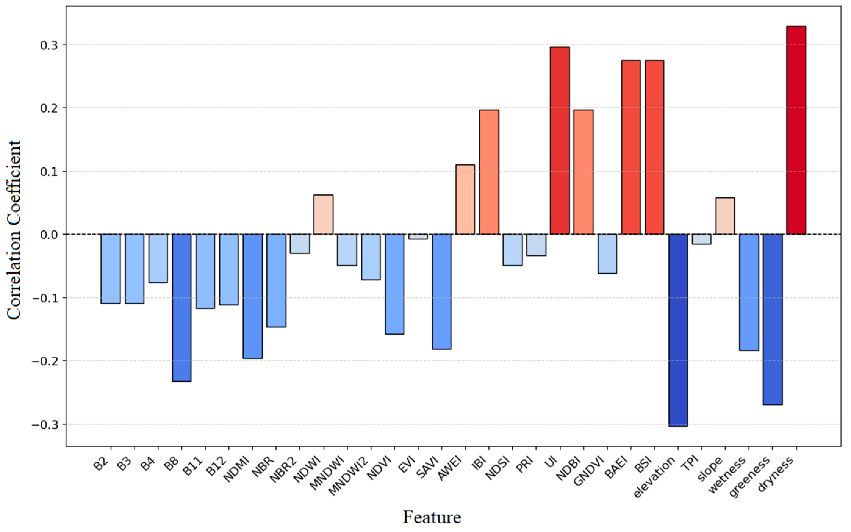
The dataset used for model training included spectral, topographic, and land cover features. Pearson’s correlation analysis identified dryness as the feature most strongly correlated with LST. Figure 7 presents the correlation coefficients for each feature.
Deep learning models, including CNN, LSTM, and GRU, were trained and validated using these datasets. Figure 8 illustrates the training loss curves for each model during the training phase.
Similarly, Figure 9 illustrates the validation loss values for all three models.
The models were evaluated using R2 and MAE. Table 3 summarizes the results, showing that the CNN model achieved the highest R2 and the lowest MAE.
Figure 10 compares the reference LST values with predictions from the CNN model, highlighting its superior accuracy.
Feature importance analysis using the SHAP method determined the relative contribution of each predictor in the CNN model. Figure 11 presents the mean absolute SHAP values, identifying Band 12 (B12) as the most influential feature, followed by Normalized Difference Snow Index (NDSI), Band 3 (B3), and elevation.
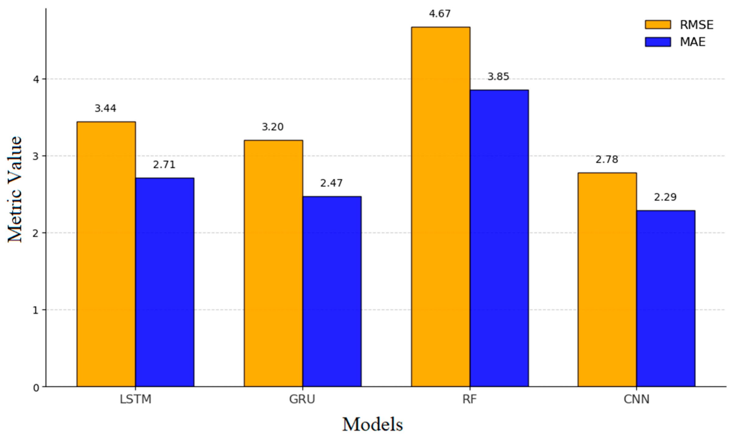
To validate model performance on test data, predictions were compared with Landsat-derived LST data, ensuring alignment with the spatial resolution. Figure 12 presents the MAE and RMSE values for the LST maps generated by each model for Tehran in July 2024.
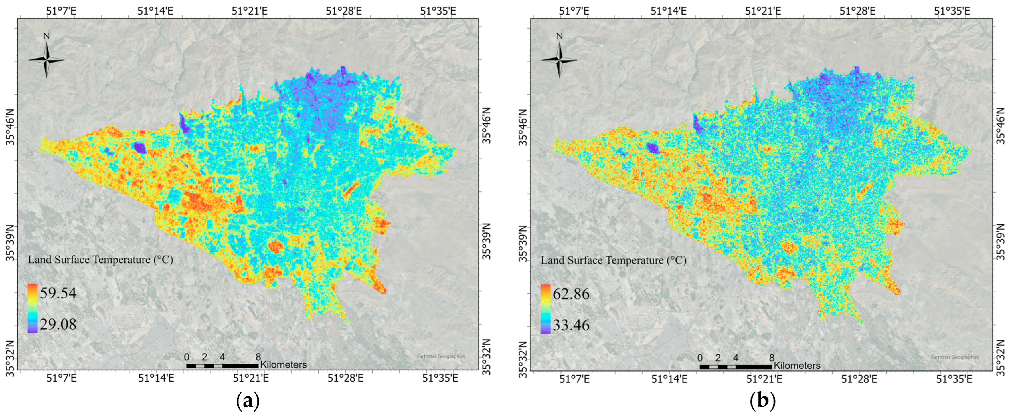
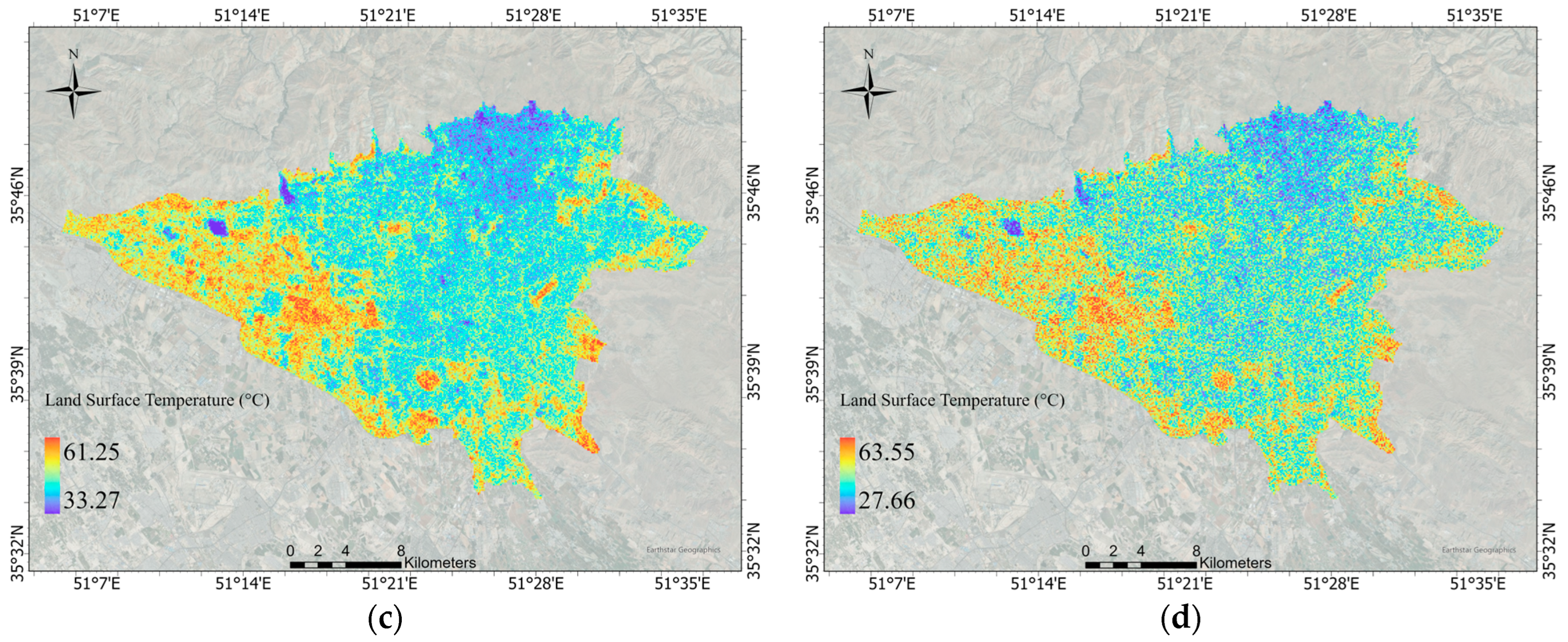
Figure 13 illustrates the LST maps generated by the CNN, LSTM, GRU, and RFR models.
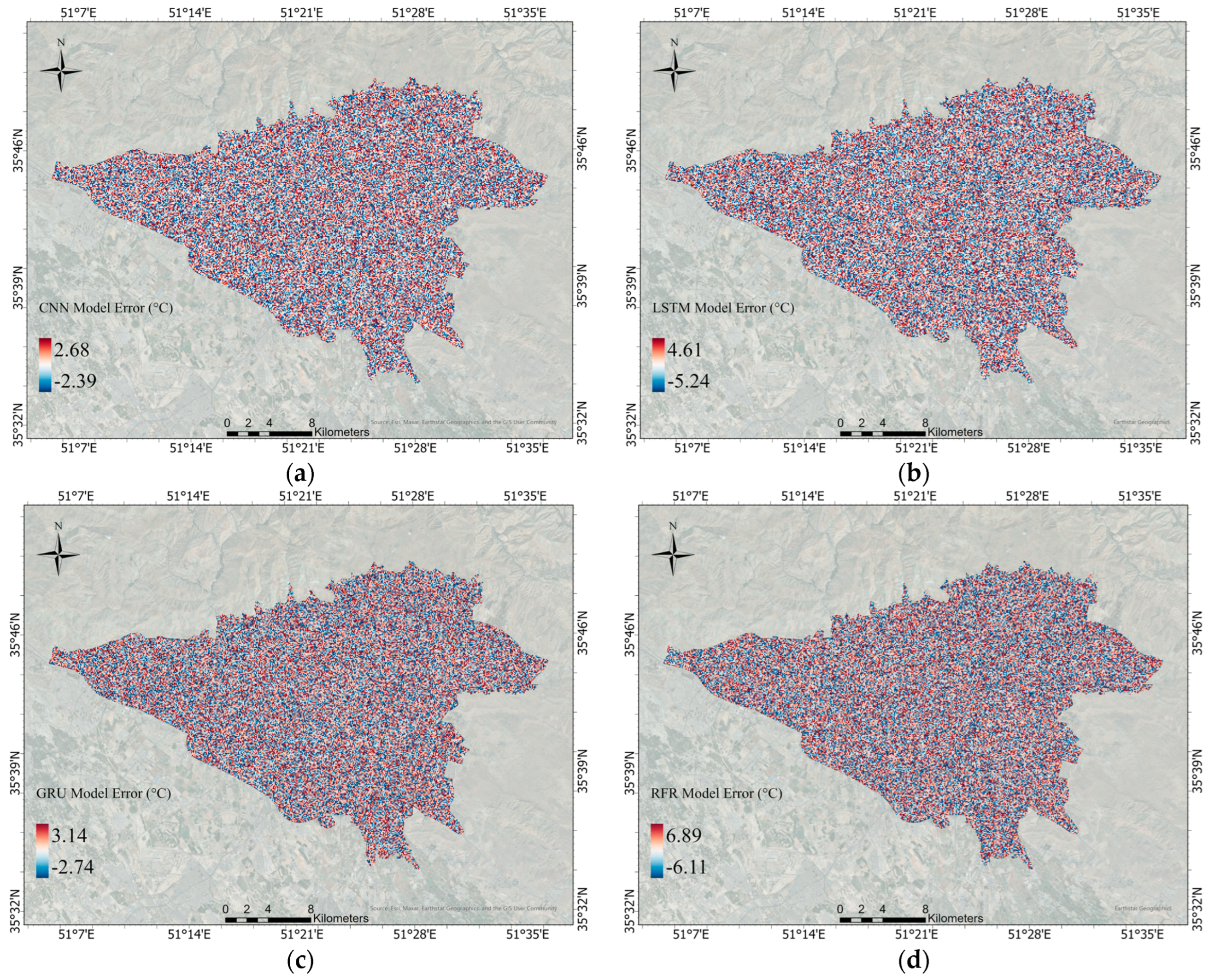
Spatial error maps were generated by computing the residuals between predicted and reference LST values. Figure 14 presents these spatial error maps, showing model accuracy variations across the study area.
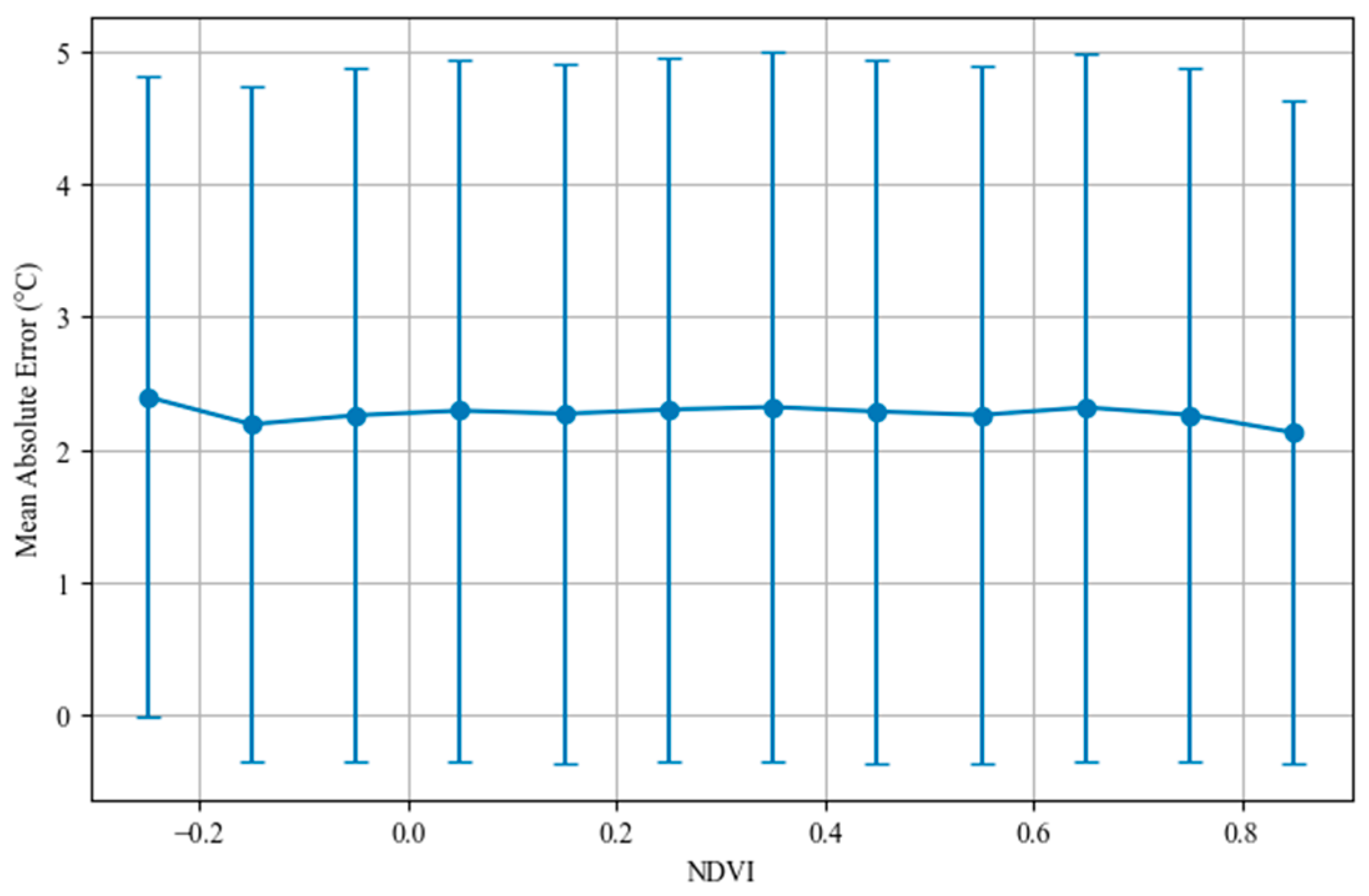
To assess the influence of land cover on prediction accuracy, an NDVI-based error analysis was conducted using the CNN model’s error map. Figure 15 illustrates the relationship between NDVI and MAE.
To further evaluate CNN model performance, the model was retrained using only the five most correlated features from Pearson’s correlation analysis. This resulted in an improved MAE of 1.19 °C and an R2 value of 84.48%. Figure 16 presents the training and validation loss trends for this optimized CNN model.
Finally, the modified TsHARP method was applied using the impervious surface fraction derived from NDBI to generate a downscaled LST map for July 2024. The method achieved an MAE of 2.6 °C and an RMSE of 3.32 °C. Figure 17 presents the downscaled LST map.

5. Discussion

The findings of this study emphasize the crucial role of input features in accurately predicting LST. Pearson’s correlation analysis identified dryness as the most strongly correlated feature with LST, underscoring its importance as a predictor. Dryness directly influences surface heat fluxes and evaporation rates, both of which are key drivers of LST variability in urban environments. Additionally, elevation and the urban index (UI) exhibited relatively strong correlations with LST, highlighting their substantial impact. Elevation affects temperature gradients through variations in atmospheric pressure and heat retention, while UI reflects urbanization levels, influencing heat generation and dissipation. The integration of these physically meaningful features enhances both model accuracy and interpretability.
This study demonstrates the effectiveness of deep learning models in predicting LST, with CNN outperforming traditional machine learning approaches. The superior performance of CNN suggests that spatial feature extraction plays a key role in accurately modeling LST patterns, particularly in heterogeneous urban environments. CNN effectively captures fine-scale spatial dependencies, making it well suited for LST estimation.
In contrast, LSTM and GRU models, which are optimized for sequential dependencies, were slightly less effective. LST variations in urban environments are primarily influenced by spatial heterogeneity—differences in land cover, urban geometry, and localized heat emissions—rather than abrupt temporal fluctuations. Consequently, CNN performs better than models focused on sequential data. Its ability to recognize complex land surface properties and impervious surface structures is particularly beneficial in dense urban landscapes.
SHAP feature importance analysis further confirmed that shortwave and near-infrared spectral bands (e.g., B12 and B8) play a crucial role in LST estimation, reinforcing the significance of spectral reflectance in detecting urban thermal variations. Additionally, NDSI was identified as an influential predictor, highlighting the role of impervious surface reflectance and bare soil properties in determining LST. In contrast, vegetation indices such as EVI had a lower impact, suggesting that in highly built-up areas, vegetation plays a relatively minor role in urban temperature regulation. These findings align with previous studies that indicate that impervious surfaces and land cover properties exert a stronger influence on LST than vegetation-related factors in dense urban settings.
The spatial error analysis reinforced the influence of land cover on model performance. The CNN model exhibited relatively stable errors across different NDVI values, with a slight reduction in error for higher NDVI levels. This aligns with the expectation that vegetated areas stabilize thermal properties through evapotranspiration and reduced surface heat retention. However, higher variability in prediction accuracy was observed in regions with low NDVI or highly heterogeneous land cover. This variability may stem from mixed land cover types, sensor limitations, or localized microclimatic effects not fully captured by the model.
Although CNN effectively extracts spatial features, accuracy could be further improved by incorporating additional contextual variables such as soil moisture, albedo, or sub-pixel heterogeneity. These findings highlight the role of vegetation in stabilizing surface temperature predictions and suggest potential refinements to enhance model robustness across diverse landscapes.
The modified TsHARP downscaling approach improved the spatial resolution of LST maps but performed worse than the CNN model. The higher MAE and RMSE values observed for TsHARP indicate that while traditional downscaling techniques enhance spatial detail, they do not fully capture the non-linear relationships between land surface properties and temperature variations. Unlike CNN, which learns complex feature representations, TsHARP relies on statistical transformations that may not effectively model spatially dependent environmental interactions.
These findings highlight the advantage of deep learning models in urban thermal analysis, where multiple interacting factors—such as built-up density, surface reflectance, and land cover transitions— introduce complexities that traditional downscaling methods may not fully address.
The generation of temporally enhanced LST maps using the proposed models and Sentinel-2 data demonstrates their practical applicability in environmental monitoring and urban planning. These high-resolution outputs facilitate more localized and effective decision making in rapidly urbanizing regions such as Tehran, which faces severe traffic congestion, elevated air pollution levels, and significant energy imbalances—all contributing to rising temperatures and associated public health risks. By improving the temporal resolution of LST data, this study provides a critical tool for real-time monitoring of urban thermal dynamics, supporting timely interventions during extreme temperature events and enhancing urban environmental risk management. The high-resolution LST maps can be integrated into Iran’s climate and environmental policy, informing heat mitigation strategies, including deploying green infrastructure to reduce urban heat effects, revising building and urban planning regulations to minimize heat accumulation, and developing early warning systems for extreme heat events. Such measures contribute to mitigating the urban heat island effect, supporting sustainable urban development and energy management policies.
Moreover, this study highlights the importance of integrating multiple environmental indicators into predictive models. These indicators can be further optimized in future research to enhance their ability to capture local conditions and improve model performance. The comparative analysis of different deep learning architectures, including CNN, LSTM network, and GRU, reveal that while all models improve the temporal resolution of LST maps, CNN outperforms the others in capturing the dynamic thermal behavior of urban areas.
These findings not only refine temporal data acquisition in remote sensing but also provide tangible benefits for urban planning, disaster management, and climate adaptation strategies in rapidly urbanizing metropolitan areas.
Previous studies have effectively enhanced LST retrieval through spatial downscaling techniques. Wang et al. [16] and Li et al. [17] reported high R2 (0.87 to 0.918) results using regression-based and machine learning approaches, while Xu et al. [14] and Jamaluddin et al. [18] achieved similar performance (R2 ≈ 0.9) through geographically weighted models and deep neural networks. Additionally, Sattari [51] enhanced the TsHARP algorithm, integrating impervious surface indices, increasing R2 to 0.83, whereas the conventional NDVI-based approach yielded a lower value of 0.73. While these methodologies improved spatial resolution, they primarily focus on specific predictors, overlooking broader environmental factors influencing urban thermal variations. To address this limitation, the present study integrates spectral, topographic, and land cover indicators, providing a comprehensive evaluation of LST dynamics. The considerable increase in MAE and R2 values when training the CNN model with the top five correlated features further underscores the importance of feature selection tailored to study area characteristics. Therefore, future research should focus on optimizing the feature selection process based on the specific attributes of the study area to improve evaluation metrics and predictive performance.
In comparison to traditional methods, the deep learning models assessed in this study demonstrated a substantial advantage in capturing complex thermal patterns. CNN outperformed the LSTM, GRU, and RFR models, and TsHARP exhibited lower accuracy in LST retrieval. Within the scope of this study, TsHARP produced weaker results than the CNN model, reinforcing the limitations of traditional downscaling approaches in addressing the non-linear thermal variations characteristic of urban environments. These findings underscore the efficacy of deep learning models in accurately modeling LST, particularly in heterogeneous urban landscapes. While previous studies primarily focused on spatial refinement, this research highlights the necessity of enhancing temporal resolution by integrating Sentinel-2 multispectral data with Landsat 8 thermal observations. This approach effectively bridges the gap between available thermal datasets and the growing demand for frequent and reliable LST monitoring in urban settings.
Despite their strong performance, deep learning models have certain limitations. High-quality input features and substantial computational resources remain challenges for large-scale applications, necessitating optimization to improve efficiency without compromising accuracy. While the models effectively capture spatial LST variations, incorporating factors such as anthropogenic heat emissions, atmospheric pollution, and land surface emissivity could enhance their representation of urban thermal dynamics. Integrating deep learning with physically based LST retrieval models may further improve generalizability. Future research should prioritize refining model architectures, incorporating additional environmental predictors, and optimizing computational scalability for broader applicability. This study confirms CNN’ superiority in capturing complex LST patterns, offering a robust framework for urban climate analysis and heat mitigation strategies.

6. Conclusions

LST data play a crucial role in urban climatology and improving environmental management, providing critical insights into spatial temperature variations. These thermal maps are critical for analyzing urban heat island effects, optimizing resource management, and guiding sustainable urban planning. Enhancing the temporal resolution of LST data improves our ability to monitor and respond to dynamic environmental changes, particularly in densely populated and rapidly urbanizing regions.
This study effectively demonstrates the effectiveness of machine learning and deep learning models in predicting LST, addressing the challenge of accurately monitoring thermal dynamics in urban environments. By integrating Sentinel-2 spectral features with Landsat 8 LST data, the proposed methodology produced detailed, high-precision LST maps, enabling more frequent temporal monitoring necessary for localized analysis.
Among the evaluated models, CNN achieved the highest predictive accuracy, achieving an R2 value of 74.81% and an MAE of 1.588 °C, underscoring the ability of CNN to effectively capture spatial patterns within LST data. LSTM and GRU networks also performed well, with R2 values of 72.11% and 71.01%, respectively, and corresponding MAE values of 1.615 °C and 1.657 °C, respectively. These results highlight their strengths in modeling temporal dependencies over multi-year datasets. However, CNN’s superior spatial feature extraction capability provided an advantage for this specific application. In contrast, RFR showed limited effectiveness in handling high-dimensional spatial datasets. Additionally, the comparison of results confirms the superiority of CNN over the traditional TsHARP method, emphasizing the need for a comprehensive examination of LST-influencing factors.
Feature selection played a crucial role in improving predictive accuracy, with dryness, elevation, and the UI identified as key predictors. These features significantly impact surface heat fluxes, evaporation rates, and the urban heat island effect, enhancing both model interpretability and robustness. The CNN model trained using the top-correlated features achieved an MAE of 1.19 and R2 of 84.48%, demonstrating the importance of optimizing feature selection based on study area characteristics.
This study contributes to urban climatology and environmental management by enabling the generation of high-accuracy thermal maps for densely populated cities such as Tehran. The evaluation of test data show that the optimal CNN model, when combined with Sentinel-2 data, achieves an MAE of 2.29 °C, allowing for higher-frequency LST mapping. However, challenges such as high computational demands and reliance on high-quality input data underscore the need for further research. Future studies should focus on improving deep learning architecture and optimizing feature selection based on the specific requirements of each model.

Author Contributions

Conceptualization, M.N. and P.P.; Methodology, M.N., P.P., B.B. and O.G.; Data Curation, M.N.; Writing—Original Draft Preparation, M.N.; Writing—Review and Editing, P.P., B.B. and O.G.; Visualization, M.N. and O.G.; Supervision, P.P., B.B. and O.G. All authors have read and agreed to the published version of the manuscript.

Funding

Open access funding provided by University of Natural Resources and Life Sciences Vienna (BOKU).

Data Availability Statement

The data that support the findings of this study are available from the first author, M.N., upon reasonable request.

Conflicts of Interest

The authors declare no conflicts of interest.

References

  1. Mutiibwa, D.; Strachan, S.; Albright, T. Land surface temperature and surface air temperature in complex terrain. IEEE J. Sel. Top. Appl. Earth Obs. Remote Sens. 2015, 8, 4762–4774. [Google Scholar] [CrossRef]
  2. Hu, J.; Fu, Y.; Zhang, P.; Min, Q.; Gao, Z.; Wu, S.; Li, R. Satellite retrieval of microwave land surface emissivity under clear and cloudy skies in China using observations from AMSR-E and MODIS. Remote Sens. 2021, 13, 3980. [Google Scholar] [CrossRef]
  3. Crossley, J.; Polcher, J.; Cox, P.; Gedney, N.; Planton, S. Uncertainties linked to land-surface processes in climate change simulations. Clim. Dyn. 2000, 16, 949–961. [Google Scholar] [CrossRef]
  4. Weng, Q.; Lu, D.; Schubring, J. Estimation of land surface temperature–vegetation abundance relationship for urban heat island studies. Remote Sens. Environ. 2004, 89, 467–483. [Google Scholar] [CrossRef]
  5. Li, Z.-L.; Tang, B.-H.; Wu, H.; Ren, H.; Yan, G.; Wan, Z.; Trigo, I.F.; Sobrino, J.A. Satellite-derived land surface temperature: Current status and perspectives. Remote Sens. Environ. 2013, 131, 14–37. [Google Scholar] [CrossRef]
  6. Meng, X.; Cheng, J.; Guo, H.; Guo, Y.; Yao, B. Accuracy evaluation of the Landsat 9 land surface temperature product. IEEE J. Sel. Top. Appl. Earth Obs. Remote Sens. 2022, 15, 8694–8703. [Google Scholar] [CrossRef]
  7. Rozenstein, O.; Qin, Z.; Derimian, Y.; Karnieli, A. Derivation of land surface temperature for Landsat-8 TIRS using a split window algorithm. Sensors 2014, 14, 5768–5780. [Google Scholar] [CrossRef] [PubMed]
  8. Griffiths, P.; Nendel, C.; Hostert, P. Intra-annual reflectance composites from Sentinel-2 and Landsat for national-scale crop and land cover mapping. Remote Sens. Environ. 2019, 220, 135–151. [Google Scholar] [CrossRef]
  9. Bharathi, D.; Karthi, R.; Geetha, P. Blending of Landsat and Sentinel images using Multi-sensor fusion. In Journal of Physics: Conference Series; IOP Publishing: Bristol, UK, 2023; Volume 2571, p. 012008. [Google Scholar]
  10. Chang, Y.; Xiao, J.; Li, X.; Middel, A.; Zhang, Y.; Gu, Z.; Wu, Y.; He, S. Exploring diurnal thermal variations in urban local climate zones with ECOSTRESS land surface temperature data. Remote Sens. Environ. 2021, 263, 112544. [Google Scholar] [CrossRef]
  11. Alexandris, N.; Piccardo, M.; Syrris, V.; Cescatti, A.; Duveiller, G. Downscaling sub-daily Land Surface Temperature time series for monitoring heat in urban environments. In Proceedings of the EGU General Assembly Conference Abstracts, Vienna, Austria, 4–8 May 2020; EGUsphere Platform: Göttingen, Germany; p. 21094. [Google Scholar]
  12. Li, W.; Ni, L.; Li, Z.-l.; Duan, S.-B.; Wu, H. Evaluation of machine learning algorithms in spatial downscaling of MODIS land surface temperature. IEEE J. Sel. Top. Appl. Earth Obs. Remote Sens. 2019, 12, 2299–2307. [Google Scholar] [CrossRef]
  13. Ebrahimy, H.; Azadbakht, M. Downscaling MODIS land surface temperature over a heterogeneous area: An investigation of machine learning techniques, feature selection, and impacts of mixed pixels. Comput. Geosci. 2019, 124, 93–102. [Google Scholar] [CrossRef]
  14. Xu, S.; Zhao, Q.; Yin, K.; He, G.; Zhang, Z.; Wang, G.; Wen, M.; Zhang, N. Spatial downscaling of land surface temperature based on a multi-factor geographically weighted machine learning model. Remote Sens. 2021, 13, 1186. [Google Scholar] [CrossRef]
  15. Yin, Z.; Wu, P.; Foody, G.M.; Wu, Y.; Liu, Z.; Du, Y.; Ling, F. Spatiotemporal fusion of land surface temperature based on a convolutional neural network. IEEE Trans. Geosci. Remote Sens. 2020, 59, 1808–1822. [Google Scholar] [CrossRef]
  16. Wang, N.; Tian, J.; Su, S.; Tian, Q. A Downscaling Method Based on MODIS Product for Hourly ERA5 Reanalysis of Land Surface Temperature. Remote Sens. 2023, 15, 4441. [Google Scholar] [CrossRef]
  17. Li, X.; He, X.; Pan, X. Application of Gaofen-6 images in the downscaling of land surface temperatures. Remote Sens. 2022, 14, 2307. [Google Scholar] [CrossRef]
  18. Jamaluddin, I.; Chen, Y.-N.; Mahendra, W.K.; Awanda, D. Deep neural network regression for estimating land surface temperature at 10 meter spatial resolution using Landsat-8 and Sentinel-2 data. In Proceedings of the Seventh Geoinformation Science Symposium, Yogyakarta, Indonesia, 25–28 October 2021; SPIE: Bellingham, WA, USA, 2021; Volume 12082, pp. 31–41. [Google Scholar]
  19. Li, W.; Ni, L.; Li, Z.-L.; Wu, H. Downscaling land surface temperature by using random forest regression algorithm. In Proceedings of the IGARSS 2018–2018 IEEE International Geoscience and Remote Sensing Symposium, Valencia, Spain, 22–27 July 2018; IEEE: New York, NY, USA, 2018; pp. 2527–2530. [Google Scholar]
  20. Wang, F.; Qin, Z.; Song, C.; Tu, L.; Karnieli, A.; Zhao, S. An improved mono-window algorithm for land surface temperature retrieval from Landsat 8 thermal infrared sensor data. Remote Sens. 2015, 7, 4268–4289. [Google Scholar] [CrossRef]
  21. Wang, L.; Lu, Y.; Yao, Y. Comparison of three algorithms for the retrieval of land surface temperature from Landsat 8 images. Sensors 2019, 19, 5049. [Google Scholar] [CrossRef]
  22. Shen, Y.; Wang, Y.; Lv, H. Thin cloud removal for Landsat 8 OLI data using independent component analysis. In Proceedings of the 2015 IEEE International Geoscience and Remote Sensing Symposium (IGARSS), Milan, Italy, 26–31 July 2015; IEEE: New York, NY, USA; pp. 921–924. [Google Scholar]
  23. Louis, J.; Pflug, B.; Debaecker, V.; Mueller-Wilm, U.; Iannone, R.Q.; Boccia, V.; Gascon, F. Evolutions of Sentinel-2 Level-2A cloud masking algorithm Sen2Cor prototype first results. In Proceedings of the 2021 IEEE international geoscience and remote sensing symposium IGARSS, Brussels, Belgium, 11–16 July 2021; IEEE: New York, NY, USA; pp. 3041–3044. [Google Scholar]
  24. Immitzer, M.; Vuolo, F.; Atzberger, C. First experience with Sentinel-2 data for crop and tree species classifications in central Europe. Remote Sens. 2016, 8, 166. [Google Scholar] [CrossRef]
  25. Wang, Z.; Sun, Y.; Zhang, T.; Ren, H.; Qin, Q. Optimization of spectral indices for the estimation of leaf area index based on Sentinel-2 multispectral imagery. In Proceedings of the IGARSS 2018-2018 IEEE International Geoscience and Remote Sensing Symposium, Valencia, Spain, 22–27 July 2018; IEEE: New York, NY, USA; pp. 5441–5444. [Google Scholar]
  26. Imran, A.; Khan, K.; Ali, N.; Ahmad, N.; Ali, A.; Shah, K. Narrow band based and broadband derived vegetation indices using Sentinel-2 Imagery to estimate vegetation biomass. Glob. J. Environ. Sci. Manag. 2020, 6, 97–108. [Google Scholar]
  27. Jiang, W.; Ni, Y.; Pang, Z.; Li, X.; Ju, H.; He, G.; Lv, J.; Yang, K.; Fu, J.; Qin, X. An effective water body extraction method with new water index for sentinel-2 imagery. Water 2021, 13, 1647. [Google Scholar] [CrossRef]
  28. Hu, B.; Xu, Y.; Huang, X.; Cheng, Q.; Ding, Q.; Bai, L.; Li, Y. Improving urban land cover classification with combined use of sentinel-2 and sentinel-1 imagery. ISPRS Int. J. Geo-Inf. 2021, 10, 533. [Google Scholar] [CrossRef]
  29. Alcaras, E.; Costantino, D.; Guastaferro, F.; Parente, C.; Pepe, M. Normalized Burn Ratio Plus (NBR+): A new index for Sentinel-2 imagery. Remote Sens. 2022, 14, 1727. [Google Scholar] [CrossRef]
  30. Castaldi, F.; Chabrillat, S.; Don, A.; van Wesemael, B. Soil organic carbon mapping using LUCAS topsoil database and Sentinel-2 data: An approach to reduce soil moisture and crop residue effects. Remote Sens. 2019, 11, 2121. [Google Scholar] [CrossRef]
  31. Lefebvre, A.; Sannier, C.; Corpetti, T. Monitoring urban areas with Sentinel-2A data: Application to the update of the Copernicus high resolution layer imperviousness degree. Remote Sens. 2016, 8, 606. [Google Scholar] [CrossRef]
  32. Le Saint, T.; Lefebvre, S.; Hubert-Moy, L.; Nabucet, J.; Adeline, K. Sensitivity analysis of Sentinel-2 data for urban tree characterization using DART model. In Proceedings of the Remote Sensing Technologies and Applications in Urban Environments VIII, Edinburgh, Scotland, 3–4 September 2023; SPIE: Bellingham, WA, USA; pp. 116–129. [Google Scholar]
  33. Phiri, D.; Simwanda, M.; Salekin, S.; Nyirenda, V.R.; Murayama, Y.; Ranagalage, M. Sentinel-2 data for land cover/use mapping: A review. Remote Sens. 2020, 12, 2291. [Google Scholar] [CrossRef]
  34. Breiman, L. Random forests. Mach. Learn. 2001, 45, 5–32. [Google Scholar] [CrossRef]
  35. Wu, H.; Li, W. Downscaling land surface temperatures using a random forest regression model with multitype predictor variables. IEEE Access 2019, 7, 21904–21916. [Google Scholar] [CrossRef]
  36. Mei, S.; Ji, J.; Bi, Q.; Hou, J.; Du, Q.; Li, W. Integrating spectral and spatial information into deep convolutional neural networks for hyperspectral classification. In Proceedings of the 2016 IEEE International Geoscience and Remote Sensing Symposium (IGARSS), Beijing, China, 10–15 July 2016; IEEE: New York, NY, USA; pp. 5067–5070. [Google Scholar]
  37. Jiang, X.; Lu, M.; Wang, S.-H. An eight-layer convolutional neural network with stochastic pooling, batch normalization and dropout for fingerspelling recognition of Chinese sign language. Multimed. Tools Appl. 2020, 79, 15697–15715. [Google Scholar] [CrossRef]
  38. Akila Agnes, S.; Anitha, J. Analyzing the effect of optimization strategies in deep convolutional neural network. In Nature Inspired Optimization Techniques for Image Processing Applications; Springer: Berlin/Heidelberg, Germany, 2019; pp. 235–253. [Google Scholar]
  39. Arora, R.; Basu, A.; Mianjy, P.; Mukherjee, A. Understanding deep neural networks with rectified linear units. arXiv 2016, arXiv:1611.01491. [Google Scholar]
  40. Garbin, C.; Zhu, X.; Marques, O. Dropout vs. batch normalization: An empirical study of their impact to deep learning. Multimed. Tools Appl. 2020, 79, 12777–12815. [Google Scholar] [CrossRef]
  41. Wang, Q.; Peng, R.-Q.; Wang, J.-Q.; Li, Z.; Qu, H.-B. NEWLSTM: An optimized long short-term memory language model for sequence prediction. IEEE Access 2020, 8, 65395–65401. [Google Scholar] [CrossRef]
  42. Van Houdt, G.; Mosquera, C.; Nápoles, G. A review on the long short-term memory model. Artif. Intell. Rev. 2020, 53, 5929–5955. [Google Scholar] [CrossRef]
  43. Ghojogh, B.; Ghodsi, A. Recurrent neural networks and long short-term memory networks: Tutorial and survey. arXiv 2023, arXiv:2304.11461. [Google Scholar] [CrossRef]
  44. Boardman, J.W.; Xie, Y. Radically Simplifying Gated Recurrent Architectures Without Loss of Performance. In Proceedings of the 2019 IEEE International Conference on Big Data (Big Data), Los Angeles, CA, USA, 9–12 December 2019; IEEE: New York, NY, USA; pp. 2615–2623. [Google Scholar]
  45. Lu, Y.; Salem, F.M. Simplified gating in long short-term memory (lstm) recurrent neural networks. In Proceedings of the 2017 IEEE 60th international midwest symposium on circuits and systems (MWSCAS), Boston, MA, USA, 6–9 August 2017; IEEE: New York, NY, USA; pp. 1601–1604. [Google Scholar]
  46. Ramadhan, M.M.; Sitanggang, I.S.; Nasution, F.R.; Ghifari, A. Parameter tuning in random forest based on grid search method for gender classification based on voice frequency. DEStech Trans. Comput. Sci. Eng. 2017, 10. [Google Scholar] [CrossRef]
  47. Agarap, A. Deep learning using rectified linear units (relu). arXiv 2018, arXiv:1803.08375. [Google Scholar]
  48. Agostinelli, F. Learning activation functions to improve deep neural networks. arXiv 2014, arXiv:1412.6830. [Google Scholar]
  49. Bock, S.; Goppold, J.; Weiß, M. An improvement of the convergence proof of the ADAM-Optimizer. arXiv 2018, arXiv:1804.10587. [Google Scholar] [CrossRef]
  50. Hu, L.; Wang, K. Computing SHAP Efficiently Using Model Structure Information. arXiv 2023, arXiv:2309.02417. [Google Scholar] [CrossRef]
  51. Sattari, F.; Hashim, M.; Sookhak, M.; Banihashemi, S.; Pour, A.B. Assessment of the TsHARP method for spatial downscaling of land surface temperature over urban regions. Urban Clim. 2022, 45, 101265. [Google Scholar] [CrossRef]
  52. Ly, A.; Marsman, M.; Wagenmakers, E.J. Analytic posteriors for Pearson’s correlation coefficient. Stat. Neerl. 2018, 72, 4–13. [Google Scholar] [CrossRef] [PubMed]
  53. Cheng, C.-L.; Garg, G. Coefficient of determination for multiple measurement error models. J. Multivar. Anal. 2014, 126, 137–152. [Google Scholar] [CrossRef]
  54. De Myttenaere, A.; Golden, B.; Le Grand, B.; Rossi, F. Mean absolute percentage error for regression models. Neurocomputing 2016, 192, 38–48. [Google Scholar] [CrossRef]
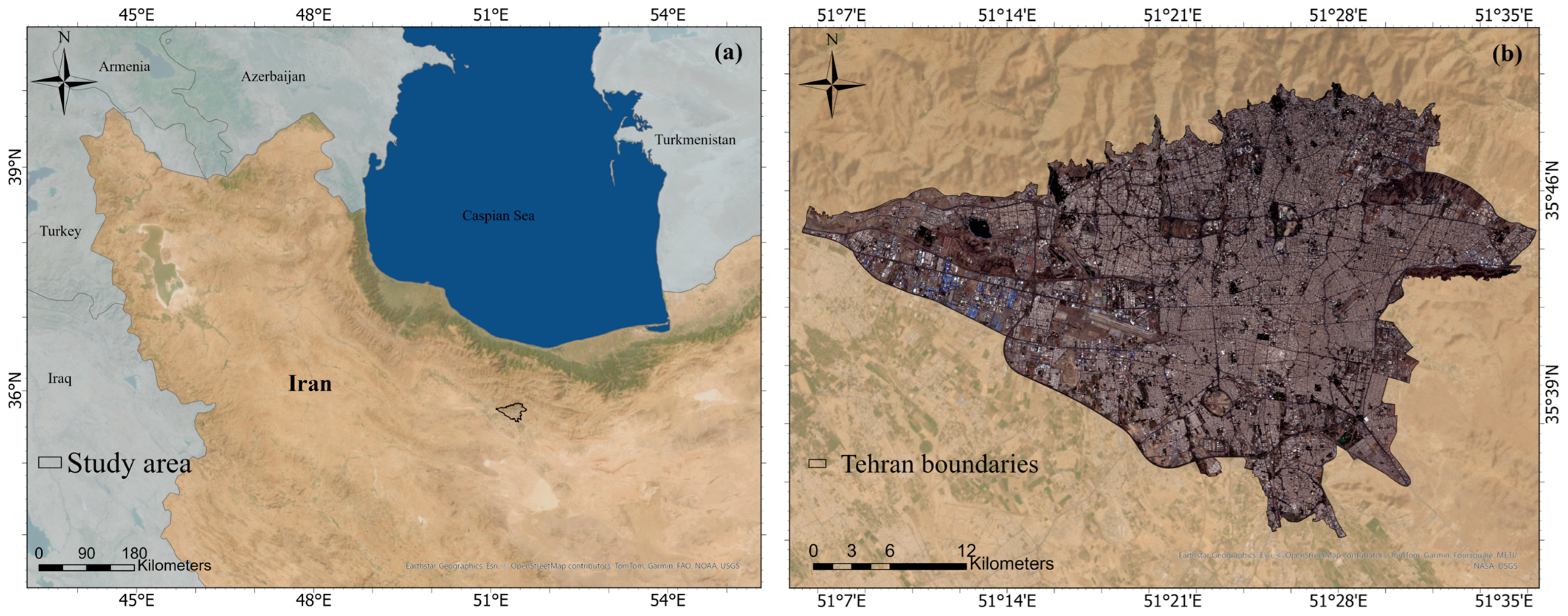
Figure 1. (a) Geographic location of the study area within Iran. (b) Spatial delineation of Tehran’s administrative boundaries and urban structure, July 2024 Methodology.
Geomatics 05 00050 g001
Figure 2. Proposed research method.
Geomatics 05 00050 g002
Figure 3. The developed CNN architecture.
Geomatics 05 00050 g003
Figure 4. LSTM model architecture.
Geomatics 05 00050 g004
Figure 5. GRU model architecture.
Geomatics 05 00050 g005
Figure 6. LST data extracted from Landsat 8 for Tehran in July 2024.
Geomatics 05 00050 g006
Figure 7. Correlation coefficients of features with the target variable.
Geomatics 05 00050 g007
Figure 8. Training loss values for (a) CNN, (b) LSTM, and (c) GRU.
Geomatics 05 00050 g008
Figure 9. Validation loss values for (a) CNN, (b) LSTM, and (c) GRU.
Geomatics 05 00050 g009
Figure 10. Actual vs. predicted LST values for the CNN model.
Geomatics 05 00050 g010
Figure 11. Mean absolute SHAP value for each feature in the CNN model.
Geomatics 05 00050 g011
Figure 12. Comparison of MAE and RMSE metrics for LST maps across different models.
Geomatics 05 00050 g012
Figure 13. LST maps of Tehran, derived using the (a) CNN, (b) LSTM, (c) GRU, and (d) RF models.
Geomatics 05 00050 g013aGeomatics 05 00050 g013b
Figure 14. Spatial error maps for (a) CNN, (b) LSTM, (c) GRU, and (d) RF models.
Geomatics 05 00050 g014
Figure 15. NDVI-based error analysis using the CNN model’s error map.
Geomatics 05 00050 g015
Figure 16. Training and validation loss trend of the CNN model with top correlated features.
Geomatics 05 00050 g016
Figure 17. LST map of Tehran, derived using the TsHARP method.
Geomatics 05 00050 g017
Table 1. Summary of features used for model training.
CategoryFeatureDescription
Spectral BandsB2, B3, B4 (Visible Bands)Blue, Green, and Red bands for vegetation, soil, and water detection [24].
B8 (NIR)Near-Infrared for vegetation vigor analysis [25].
B11, B12 (SWIR)Shortwave Infrared bands for moisture and geological analysis [26].
Spectral IndicesNDVI, EVI, SAVI, GNDVIMeasure vegetation health, density, and greenness [26].
NDWI, MNDWI, AWEI, MNDWI2Identify and enhance water body detection [27].
NDBI, UI, IBIHighlight urban and built-up areas [28].
NBR, NBR2Assess burned areas and vegetation stress [29].
BSI, PRI, BAEIIndicate soil characteristics, dryness, and photosynthetic activity [30].
NDSIHighlights snow-covered areas [31].
Topographic DataElevationHeight above sea level from digital elevation models (DEMs) [32].
TPI (Topographic Position Index)Classifies landforms based on elevation [32].
SlopeMeasures terrain steepness [32].
Land Cover DataWetness Derived from MNDWI2, indicating the presence of surface water [33].
Greenness Derived from NDMI, representing vegetated areas not classified as wet [33].
DrynessIdentifies dry surfaces as areas classified as neither wet nor green, with a smoothing filter applied [33].
Table 2. Hyperparameter search space for model tuning.
ModelHyperparameterSearch RangeSelected Value
RFRNumber of estimators100, 150, 200, 250, 300250
Maximum depth10, 20, 30, 40, None30
Minimum samples split2, 5, 105
CNNNumber of convolutional layers2, 3, 43 layers
Filters per layer64, 128, 256256, 128, 64 (from first to third layer)
Kernel size(3 × 3), (5 × 5)(3 × 3)
Batch size8, 16, 3216
Learning rate10−3, 10−4, 10−5Fine-tuned to 3.9063 × 10⁻⁶
LSTM and GRUNumber of recurrent layers2, 3, 44 layers
Units per layer64, 128, 256256, 128, 64, 32 (from first to fourth layer)
Batch size8, 16, 3216
Learning rate10−3, 10−4, 10−510−3 (initial), reduced to 10−6 upon plateau
Table 3. Validation of methods.
MethodR2MAE (Celsius)
RFR55.75%2.3818
CNN74.81%1.5880
LSTM72.11%1.6151
GRU71.01%1.6565
Disclaimer/Publisher’s Note: The statements, opinions and data contained in all publications are solely those of the individual author(s) and contributor(s) and not of MDPI and/or the editor(s). MDPI and/or the editor(s) disclaim responsibility for any injury to people or property resulting from any ideas, methods, instructions or products referred to in the content.