Abstract
Individual tree parameters are essential for forestry decision-making, supporting economic valuation, harvesting, and silvicultural operations. While extensive research exists on uniform and simply structured forests, studies addressing complex, dense, and mixed forests with highly overlapping, clustered, and multiple tree crowns remain limited. This study bridges this gap by combining structural, textural, and spectral metrics derived from unmanned aerial vehicle (UAV) Red–Green–Blue (RGB) and multispectral (MS) imagery to estimate individual tree parameters using a random forest regression model in a complex mixed conifer–broadleaf forest. Data from 255 individual trees (115 conifers, 67 Japanese oak, and 73 other broadleaf species (OBL)) were analyzed. High-resolution UAV orthomosaic enabled effective tree crown delineation and canopy height models. Combining structural, textural, and spectral metrics improved the accuracy of tree height, diameter at breast height, stem volume, basal area, and carbon stock estimates. Conifers showed high accuracy (R2 = 0.70–0.89) for all individual parameters, with a high estimate of tree height (R2 = 0.89, RMSE = 0.85 m). The accuracy of oak (R2 = 0.11–0.49) and OBL (R2 = 0.38–0.57) was improved, with OBL species achieving relatively high accuracy for basal area (R2 = 0.57, RMSE = 0.08 m2 tree−1) and volume (R2 = 0.51, RMSE = 0.27 m3 tree−1). These findings highlight the potential of UAV metrics in accurately estimating individual tree parameters in a complex mixed conifer–broadleaf forest.
1. Introduction
Individual tree parameters, such as tree height (H), diameter at breast height (DBH), basal area (BA), stem volume (V), and carbon stock (CST), are crucial for accurate forest inventories and sustainable forest management [1]. These parameters hold significant economic and ecological value, supporting the single-tree management of high-value timber species in mixed conifer–broadleaf forests [2,3,4]. Monitoring individual trees enables the assessment of tree growth and structure, biomass accumulation, and biodiversity conservation, while contributing to climate change mitigation and timber resource optimization [1,5,6]. Accurate estimation of individual tree parameters also facilities forest health monitoring by enabling early detection of tree-level stress indicators, such as reductions in H or BA growth, which can signal potential threats like pests, diseases, or environmental stressors. Such insights are essential for timely interventions and risk mitigations [7,8,9]. Additionally, precise individual parameter estimation supports adaptive management practices, such as selective thinning or regeneration planning, ensuring the long-term health, resilience, and sustainability of forest landscapes [1,8,10,11]. Therefore, individual tree parameter estimations play a pivotal role in promoting sustainable forest landscapes and informed decision-making processes [12,13].
Forest inventory using conventional methods are time-consuming, labor-intensive, inefficient, and often impractical in inaccessible areas [14,15]. Remote sensing (RS) technology offers a more efficient alternative, enabling precise estimation of individual tree parameters in mixed conifer–broadleaf forests. Advances in RS provide high-resolution forestry data and robust methodologies [1,16], improving the accuracy of monitoring individual tree growth and spatial distribution on a large scale [11,17,18,19].
While satellite imagery has been widely used to estimate forest structural parameters, its application for individual tree parameters is limited by low spatial resolution and atmospheric interference [20,21,22]. Among RS technologies, unmanned aerial vehicle (UAV) photogrammetry and light detection and ranging (LiDAR) are frequently used to obtain 3D forest information [17,23]. LiDAR is an active RS technology; emits laser beams to detect objects; and is highly effective for capturing structural details at both forest and individual tree scales, including tree height, crown dimensions, and biomass [17,22,23]. However, LiDAR sensors lack spectral information, which is critical for continuous monitoring [24,25]. To address this limitation, spectral sensors can be mounted alongside LiDAR on UAV platforms, enabling the simultaneous collection of structural and spectral data.
UAV photogrammetry is a specialized method created for 3D mapping in the RS field, and it has rapidly advanced in recent years [26,27]. Studies have shown that its accuracy in estimating individual tree parameters is comparable to that of LiDAR [28,29], with additional advantages such as low cost, repeatability, and high flexibility [23]. Structure from Motion (SfM) in UAV photogrammetry efficiently converts 2D digital aerial photographs into 3D photogrammetric point clouds [26], enabling detailed forest canopy characterization and visualization of individual tree canopies [1,30]. In dense, clustered, and highly overlapping canopy forests, UAV photogrammetry excels at identifying tree canopy edges and accurately delineating tree crowns, using rich textural features [1,31]. High-resolution imagery also reduces the likelihood of missing treetops in complex forests [30]. Moreover, UAV platforms support various sensors, enabling the collection of spectral information from Red–Blue–Green (RGB), multispectral (MS), and hyperspectral imagery [28,32], serving as an affordable supplementary data source.
Advancements in UAV photogrammetry have enabled accurate prediction of individual tree parameters in simple-structured, even-aged, sparse forests. However, challenges persist in dense, clustered, complex, mixed, and highly overlapped forests due to missing crown information [12,14,33]. Moe et al. [4] reported a correlation of 0.68 for H accuracy between field measurement and UAV RGB photogrammetry in a mixed conifer–broadleaf forest with high-valued timber species. Accuracy varied across the species: castor aralia had the highest H accuracy (R2 = 0.77, RMSE = 2.04 m), followed by monarch birch (R2 = 0.27, RMSE = 1.77 m) and oak (R2 = 0.10, RMSE = 1.96 m). For tree DBH, correlations between field and UAV photogrammetry were 0.72, 0.57, and 0.75 for the abovementioned species, respectively. These studies employed manual crown delineation and multiresolution segmentation for individual tree parameter estimation. Data fusion approaches using LiDAR and optical sensors for biomass (R2 = 0.33–0.82) and volume (R2 = 0.39–0.87) estimation have shown a wide range of accuracy [25]. Zhao et al. [11] achieved high accuracy for H in coniferous forests (R2 = 0.87, RMSE = 0.21 m), followed by mixed conifer–broadleaf forest (R2 = 0.84, RMSE = 0.37 m) and broadleaf forests (R2 = 0.84, RMSE = 0.44 m), using LiDAR data. However, studies on estimating individual tree parameters in complex, dense, and mixed forests using UAV photogrammetry remain limited.
Structural, spectral, and textural metrics derived from point clouds and imagery have been used to estimate individual tree parameters [28,34,35]. Combining UAV remote-sensing variables such as structural, textural, and spectral metrics generally improves accuracy in estimating forest structural parameters using UAV RGB imagery [18]. Textural information is particularly important for capturing spatial details of forest structural arrangements [18,34]. In a previous study [28], we estimated the forest structural parameters at stand level using a combination of these metrics derived from UAV RGB imagery in mixed conifer–broadleaf forests. The results showed that combining these metrics enhanced the estimation accuracy of H, DBH, BA, V, and CST using a random forest (RF) model. However, using this for estimating individual tree parameters in mixed conifer–broadleaf forests is limited. Spectral metrics from MS imagery have been used for tree species classification [11,19,36,37], but their use for estimating individual tree parameters in mixed forests is underexplored. Moreover, most studies focus on H and DBH, with limited exploration of tree BA, V, and CST in complex forests. While area-based forest structural parameters provide high accuracy [28], accurately predicting individual tree parameters in complex mixed conifer–broadleaf forests remains challenging. This study extends previous work by estimating the same parameters (H, DBH, BA, V, and CST) at the individual tree level using a combination of structural, textural, and spectral metrics from both UAV RGB and MS imagery in mixed conifer–broadleaf forests. The key difference is the scale of parameter analysis at the individual tree level, along with the integration of MS imagery.
Given the challenges in predicting individual tree parameters in mixed conifer–broadleaf forests, we aimed to combine UAV metrics, comprising structural, textural, and spectral metrics. Structural and textural metrics were extracted from the canopy height model (CHM), while spectral metrics were derived from RGB and MS imagery. An RF model was used to estimate individual tree parameters. The research questions guiding this study are as follows: (1) Can high-resolution UAV orthomosaic enable the accurate delineation of individual tree crowns and CHM generation in mixed conifer–broadleaf forest? (2) Which UAV metrics are most important for predicting individual tree parameters in this forest? (3) Can UAV photogrammetry improve the estimation accuracy of H, DBH, BA, V, and CST for conifer, oak and other broadleaf (OBL) species by combining UAV metrics from UAV RGB and MS imagery? Our approach significantly aids forestry practitioners in estimating individual tree parameters in complex mixed conifer–broadleaf forests. The application of high-resolution UAV imagery assists in delineating individual tree species. By integrating UAV-derived metrics from RGB and multispectral (MS) imagery, we provide accurate individual tree parameters that support forest inventory efforts. Traditional ground surveys are time-consuming and labor-intensive, making frequent data collection impractical. In contrast, our approach enables data collection at any time using UAV photogrammetry, reducing the burden of conventional surveys. This integrated method highlights the importance of individual tree parameter estimation, particularly in complex forest environments.
2. Materials and Methods
2.1. Study Site
This study was carried out at the University of Tokyo Hokkaido Forest (UTHF), located at 43°10–20′ N, 142°18–40′ E, and 190–1459 m asl, in Furano City in Hokkaido, Northern Japan (Figure 1). UTHF is an uneven-aged, hemiboreal, and mixed conifer–broadleaf forest situated between temperate deciduous and boreal evergreen coniferous forests, encompassing an area of 22,708 ha. Dominant conifer species include Abies sachalinensis (Todo fir), P. glehnii (red spruce), and Picea jezoensis (Yezo spruce), while dominant broadleaf species are Quercus crispula (oak), Betula maximowicziana (Monarch birch), Kalopanax septemlobus (castor aralia), Acer pictum (Painted maple), Tilia japonica (linden), Fraxinus mandshurica (Manchurian ash), and Taxus cuspidata. Dwarf bamboo species, Sasa kurilensis and S. senanensis, cover the forest floor. From 2001 to 2008, the arboretum’s average annual temperature was 6.4 °C, with annual rainfall totaling 1297 mm at the elevation of 230 m asl. The forest floor is snow-covered from November to April, with snow accumulation reaching up to 1 m [2,28]. The study site, forest sub-compartment 68 E, was selected due to its high distribution of oak, high-valued timber species, particularly for whisky barrel production. Conifers, oak, and other broadleaf (OBL) species were categorized for the study. The study area spans 31 ha, with elevations ranging from 425 m to 500 m asl [38]. The study site has a mean tree density of 562 stems ha−1 (DBH ≥ 5 cm, standard deviation = 73 stems ha−1, range = 460–656 stems ha−1) based on five inventory plots, each with a dimension of 50 m × 50 m (source: UTHF 2020 inventory data, March).
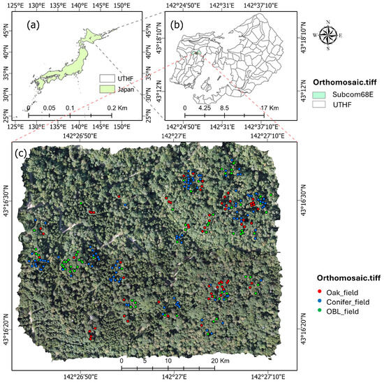
Figure 1.
Study area map: (a) location of the UTHF in Japan; (b) sub-compartment 68 E in the UTHF; and (c) spatial tree location of oak, conifer, and other broadleaf (OBL) species in the UAV orthomosaic.
2.2. Collection of Field Data
A field survey was conducted in February 2023 to measure tree geospatial positions, H, and DBH. To identify the spatial position of dominant trees (≥24 m) prior to the field survey, we used a freely available web application by Silva et al. [39] (https://carlosasilva.shinyapps.io/weblidar-treetop/, accessed on 15 January 2023) which reduced field work time. Trees were randomly selected across the study area (Figure 1c). Geospatial positions of trees were recorded using a real-time kinematic (RTK) system of global navigation satellite system (GNSS) with a dual-frequency receiver (DG-PRO1RWS, BizStation Corp., Matsumoto City, Japan). In total, 255 trees were identified, comprising 115 conifers, 67 Japanese oak, and 73 OBL species. DBH was measured with a diameter tape at 1.3 m from the ground floor, and BA was calculated based on DBH. H measurements focused on conifers, as broadleaf trees had shed their leaves during the survey, improving the visibility of conifer treetops. H was measured three times, using a Vertex III hypsometer (Haglöf Sweden AB, Långsele, Sweden), and the average value was recorded. For the conifer H prediction, only 52 field-measured trees were used, while 115 trees were utilized for other individual tree parameters. H measurements for oak and OBL were not conducted due to overlapping canopies and multiple tree crowns, which are characteristic of complex forests. Instead, H for these species was estimated using a H-DBH model, a widely adopted method H prediction [40,41,42]. A nonlinear regression model (Equation (1)) was applied to derive the H-DBH relationship [42,43], based on measurements from 216 trees (oak and OBL) in other forest compartments (16, 65–66, and 03) recorded during the UTHF 2023 field survey.
where 1.3 is a measuring height of DBH from ground floor, and a and b are model parameters. The values of a and b were 7.29 and 0.3, respectively. Model r, R2, and RMSE were 0.6, 0.37, and 3.22 m, respectively (Figure A1).
The one-variable volume equation derived from DBH was used to derive the V of individual trees for the UTHF. The V equation (Equation (2)) was used for conifer species in UTHF [44]. V tariffs for broadleaf species are based on Equations (3) and (4), used for Fraxinus spp. with DBH < 80 cm and DBH ≥ 80 cm, respectively. Similarly, Equations (5) and (6) were used for OBL species with DBH < 80 cm and DBH ≥ 80 cm, respectively [45]. CST was estimated using the allometric equation (Equation (7)) [46]:
where d—DBH; V—stem volume for a species (m3 tree−1); CST—carbon stock for a species (MgC tree−1); D—wood density (t–d.m. m–3); CF—dry-matter carbon fraction (MgC t–d.m.–1); BEF—biomass expansion factor; R—root-to-shoot ratio; and j—tree species [46]. Table 1 shows the field data results.

Table 1.
Mean value of the individual tree parameters.
2.3. Collection of UAV Imagery
Table 2 provides detailed information on flight parameters, UAV platforms, and sensor specifications for RGB and MS imagery collection. A DJI Matrice 300 RTK was flown to capture RGB imagery during leaf-on (October) and leaf-fall (November) seasons in 2022. In 2023, a DJI Mavic 3 Multispectral (3M) with RTK was used to capture both RGB and MS imagery during leaf-on season. Imagery collection in October for both years ensured consistency in seasonal timing. A square parallel flight plan was predesigned (Figure A2). The UAV RGB imagery collected on 8 November 2023, during the leaf fall season, was solely used for visually identifying tree species and not for metric extractions. All data collection was performed on sunny days with clear atmospheric conditions [38].
Table 2.
Flight parameters and specifications for RGB and MS imagery collections using DJI Matric 300 RTK and DJI Mavic 3M RTK.
In mixed forests, spectral variations and shadows within heterogeneous tree crowns can result in segmentation errors, where a single tree crown may be erroneously divided into multiple crowns [4,42]. To mitigate this, the Mavic 3M drone simultaneously collected RGB and MS imagery in a single flight, ensuring consistency and eliminating shadow and illumination differences. The MS imagery captured spectral bands, including red (R), green (G), red edge (RE), and near-infrared (NIR). A total of 2798 images were collected for Mavic RGB imagery, and 3138 images were collected for Matice RGB imagery. For MS imagery, 11,192 images were collected. Unclear and blurred images were removed for the image processing. The ground resolutions for RGB and MS imagery were 1.61 cm/pixel and 2.8 cm/pixel, respectively, with reprojection errors of 1.81 pixels for RGB and 0.60 pixels for MS imagery. Geolocation errors were 2.91 cm for RGB and 1.68 cm for MS imagery. Direct georeferencing of UAV imagery was performed without ground control points due to the dual-frequency RTK GNSS capability of UAV. This system provides highly accurate real-time location data by using satellite signals and correction data from a base station. The dual-frequency feature further improved precision by correcting for atmospheric interference, achieving centimeter-level accuracy, consistent with the findings of Htun et al. [38].
2.4. Data Analysis
2.4.1. Processing UAV Images
Figure 2 outlines the study workflow. UAV imagery was processed by the staff of UTHF using Agisoft Metashape version 1.8.4 (Agisoft LLC, St. Petersburg, Russia) and Pix4Dmapper version 4.8.0 (Lausanne, Switzerland). Sensor correction, camera calibration, and reflectance panel calibration were conducted using the respective software. Pixel values of orthomosaic images were used for analysis. Original resolutions of 0.08 m/pixel for the DJI Terra RGB orthomosaic and 0.02 m/pixel for both the DJI Mavic RGB and MS orthomosaics were resampled to 0.5 m/pixel. This resampling was performed to reduce computational load and ensure resolution consistency when combining the imagery with the CHM and Digital Terrain Model (DTM) for individual tree parameter estimation. The accuracy of the UAV-derived DTM was constrained by canopy obstruction. Therefore, a high-precision DTM was utilized, derived from an Optech ALTM Orion M300 LiDAR sensor (Teledyne Technologies, Thousand Oaks, CA, USA) attached to a helicopter in 2018, and this approach is consistent with previous studies [4,28]. This provided more accurate information on the vertical forest structure [29]. The CHM for the DJI Terra RGB flight was generated by deducting the LiDAR-derived DTM from the UAV-derived Digital Surface Model (DSM). The LiDAR DTM provided by UTHF was instrumental in this procedure [28,29]. The terrain of the forest floor remains relatively consistent over time; therefore, we used the LiDAR DTM obtained in 2018. However, since tree growth has increased over time, we used the UAV DSM to estimate the CHM in the absence of a recent LiDAR DTM for this study area. The RMSE and standard deviation of the LiDAR DTM were both 0.061 m. This indicates that both the UAV data and LiDAR DTM had low reprojection and geolocation errors, ensuring spatial consistency between them. In addition, we used spatial resolutions of 0.5 m/pixel for LiDAR DTM and UAV DSM for spatial consistency.
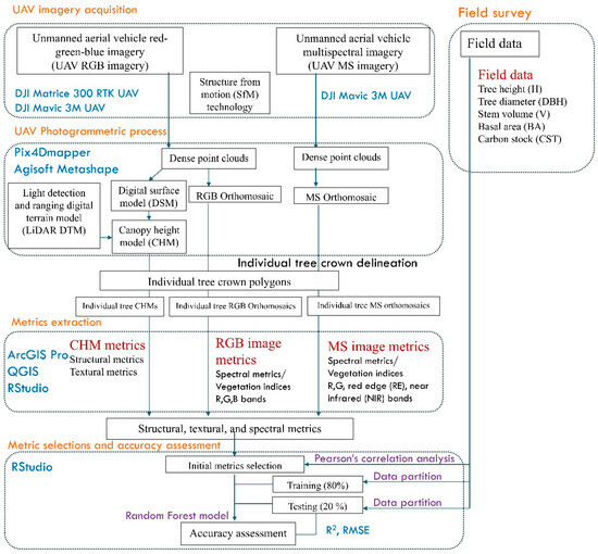
Figure 2.
The study workflow included field data enumeration, UAV photogrammetry, CHM generation, and feature extraction from CHM and orthomosaic metrics. UAV—unmanned aerial vehicle; RGB—Red–Green–Blue; MS—multispectral; DSM—Digital Surface Model; SfM—Structure-from-Motion technology; RE—red edge; NIR—near-infrared.
2.4.2. Tree Crown Delineation
The spatial locations of field-measured trees, combined with visual observation of tree crowns in the UAV orthomosaic, enabled manual delineation of individual tree crowns. A high-resolution (0.8 cm/pixel) UAV RGB orthomosaic was used for clear identification where tree crown edges were more visible. Delineation was conducted using DJI Matrice RGB imagery (2022) and DJI Mavic RGB imagery (2023). Visual comparison of the tree polygons from both years showed consistent results. A paired t-test (p < 0.05) confirmed no significant difference in crown area (CA) between the two datasets. Therefore, tree polygons derived from the DJI Matrice RGB orthomosaic were used for metric extraction, as they were closer to the field data collection period. Tree crown delineation was straightforward for single-stem conifers but more challenging for clustered or multi-crown trees, particularly oak and other broadleaf species. Orthomosaic imagery collected during the leaf-fall season improved identification by revealing branches and upper stems, aiding in delineation in clustered canopy areas (Figure A3). Manual delineation took approximately 86 min for conifers (n = 115), 52 min for oak (n = 67), and 54 min for OBL (n = 73), with an average time of 46–80 s per tree crown. This included simultaneous observation of the CHM. Identifying individual tree crowns in MS orthomosaic was more challenging due to the visibility limitations of the green and red bands (Figure A4).
2.4.3. Extraction of Metrics from CHM and Orthomosaics
Table 3 summarizes the UAV-derived structural, textural, and spectral metrics. Manually delineated tree crown polygons were used to assess individual tree parameters due to the presence of multiple highly overlapping tree crowns. These polygons served as the reference for feature extraction. Structural and textural metrics were extracted from CHM (7 October 2022), while spectral metrics were derived from RGB and MS orthomosaics (27 October 2023). Spectral metrics are the vegetation indices measured by the light reflectance across wavelengths [47]. These are crucial tools in RS, providing insights into the health, structure, and productivity of vegetation across landscapes [48,49]. In forest management and inventory, spectral metrics help quantify forest attributes [49]. RGB spectral metrics are derived from R, G, and B bands, while MS spectral metrics are derived from R, G, RE, and NIR bands. The normalized difference vegetation index (NDVI) measures the reaction to chlorophyll content that resamples the vegetation growth and nutrients. Green NDVI (GNDVI) indicates the amount of water or nutrients that indicates the biomass. Leaf chlorophyll content (LCI) is related to vegetation growth and yield, disease, growth, aging, and physiological disorders. The normalized difference red edge index (NDRE) indicates the variation of chlorophyll and sugar content [34]. Textual metrics were calculated using the gray-level co-occurrence matrix (GLCM), which evaluates pixels’ brightness variations in the CHM [35] to detect differences in gray levels [50,51] (Figure A5). Structural metrics such as mean, standard deviation (std), and maximum of CHM and CA values were calculated using ArcGIS Pro statistics. Textural metrics were derived with the r.texture algorithm in QGIS version 3.28 using a 3 m × 3 m window size for individual tree parameter estimation.
Table 3.
The metrics derived from CHMs and RGB orthomosaics.
2.4.4. Random Forest Estimation and Accuracy Assessment
Individual tree parameters measured in the field were compared with structural, textural, and spectral metrics, as well as their combination, using the RF regression model. The RF algorithm is widely employed in RS due to its robustness and capacity to handle randomness [65]. The RF model was applied using the “randomForest” package (version 4.7–1.1) in RStudio version 4.22. Key parameters such as mtry and ntree were optimized within the model [28,53] to achieve the high R2 and low RMSE. Metrics were ranked by their importance using the percent increase in mean squared error (%IncMSE) and in node purity (IncNodePurity). %IncMSE was prioritized for metric selection. The error tends to increase when random variables are substituted.
Despite the usage of a large number of variables, identifying the most important structural, textural, and spectral metrics is crucial. Dimensionality reduction is essential for selecting relevant RS metrics and avoiding multicollinearity. To address the multicollinearity and identify the most relevant RS metrics, a two-step approach was applied: Firstly, we performed the Pearson’s correlation test using the “metan” package. Metrics negatively correlated (p at 0.05) with field-measured individual tree parameters were removed [28]. Secondly, category-specific RF analysis was performed. Structural, textural, and spectral metrics were analyzed in the RF model to eliminate the least important metrics. The most important metrics from each category were combined, and the top ten metrics were selected through further RF analysis. The RF model also inherently performs dimensionality reduction through out-of-bag (OOB) validation, ranking variable importance [66]. The dataset was split into training (80%) and testing (20%). The model was fine-tuned by iteratively removing the least important metrics to achieve the best accuracy, and the final set of metrics was chosen for estimating individual tree parameters. RMSE and R2 were used together for prediction accuracy [67].
3. Results
3.1. The Tree Crown Delineation and CHM Extraction
Figure 3 illustrates the results of individual tree crown delineation and CHM extraction for conifer, oak, and OBL species. The mean CA for conifer, oak, and OBL was 37.11 ± 16.12 m2 (n = 115), 121.78 ± 49.88 m2 (n = 67), and 66.96 ± 46.08 m2 (n = 73), respectively. The CHM accuracy was evaluated by comparing CHM maximum with field-measured H of conifer trees. The comparison showed high accuracy (R2 = 0.86, r = 0.93, RMSE = 2.15 m, %RMSE = 7.68, n = 52; Figure 3c).
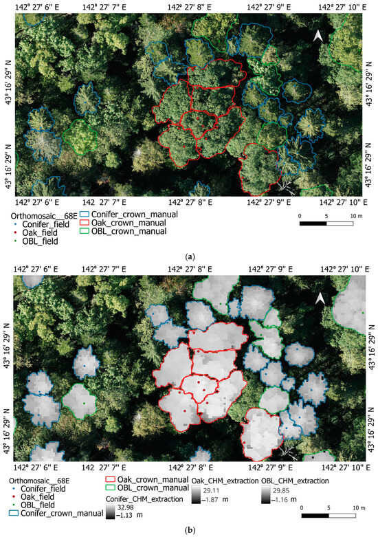
Figure 3.
The individual tree crown delineation and CHM extraction of conifer, oak, and OBL with the field tree geospatial location: (a) manual crown delineation of conifer, oak, and OBL; (b) individual CHM extraction of conifer, oak, and OBL with the field tree geospatial location. (c) A linear relationship between conifer field tree height (H) and canopy height maximum (CHM max).
3.2. Variable Selection for Individual Tree Parameters
Figure 4 displays the top ten metrics, along with the final selected metrics by the RF model, using a combination of structural, textural, and spectral metrics. CA was the most significant metric for predicting individual parameters (H, DBH, BA, V, and CST). For conifer H prediction, structural (CHM max and CHM mean), textural (SA, ASM, and SV), and spectral metrics (NDVI, GNDVI, and G_R) were selected. Structural metrics such as CHM max, CHM mean, and CA had the greatest contribution to estimating individual tree parameters, followed by textural and spectral metrics (Figure 4, first row). For oak and OBL H prediction, CA and CHM std were important structural metrics, with additional contribution from textural and spectral metrics. For oak, CA contributed to estimating DBH and BA, while CA and CHM_std were important for V and CST. For OBL, CA and textural metrics contributed to estimating DBH, BA, V, and CST, with spectral metrics excluded in some cases.
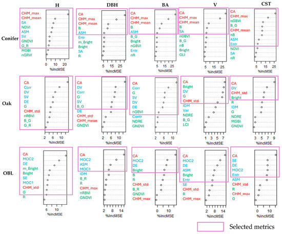
Figure 4.
The top ten UAV metrics with finally selected metrics (purple box) by RF model in combined metrics from structural (red-color font), textural (blue-color font), and spectral metrics (green-color font): left to right, RF model column shows variable importance selection for H, DBH, BA, V, and CST. From top to bottom, rows show the results of variable-importance selection for conifer, oak, and OBL.
3.3. Accuracy of Individual Tree Parameters
Table 4 presents the accuracy of individual tree parameters—H, DBH, BA, V, and CST—for conifer, oak, and OBL species using structural, textural, spectral, and combined metrics. Figure 5 compares field-measured individual tree parameters with those predicted by UAV metrics. Overall, combined metrics provided the highest accuracy for all parameters, outperforming individual metric categories. Conifer species showed higher accuracy than oak and OBL species.
Table 4.
The accuracy of individual tree parameter estimation of H, DBH, BA, V, and CST for conifer, oak, and OBL at structural, textural, spectral, and combined metrics, using RF regression model.
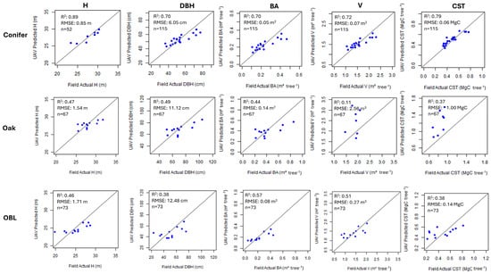
Figure 5.
The results of the field-measured individual tree parameters versus UAV-predicted individual tree parameters: From left to right, figure illustrates the individuals tree parameters of H, DBH, BA, V, and CST. From top to bottom, figure illustrates the results of individual tree parameters for conifer, oak, and OBL.
For H, combined metrics showed higher accuracy for conifer (R2 = 0.89, RMSE = 0.85 m), followed by oak (R2 = 0.47, RMSE = 1.54 m) and OBL (R2 = 0.46, RMSE = 1.71 m). Similarly, DBH accuracy was highest for conifer (R2 = 0.70, RMSE = 6.05 cm), followed by oak (R2 = 0.49, RMSE = 11.12 cm) and OBL (R2 = 0.38, RMSE = 12.48 cm). Conifer had the highest accuracy for BA (R2 = 0.70, RMSE = 0.05 m2 tree−1), followed by OBL (R2 = 0.57, RMSE = 0.08 m2 tree−1) and oak (R2 = 0.44, RMSE = 0.14 m2 tree−1). For V, conifer showed the highest accuracy (R2 = 0.72, RMSE = 0.07 m3 tree−1), followed by OBL (R2 = 0.51, RMSE = 0.27 m3 tree−1) and oak (R2 = 0.11, RMSE = 2.56 m3 tree−1). For CST, conifer had the highest accuracy (R2 = 0.79, RMSE = 0.06 MgC tree−1), followed by OBL (R2 = 0.38, RMSE = 0.14 MgC tree−1) and oak (R2 = 0.37, RMSE = 1.00 MgC tree−1).
4. Discussion
4.1. Tree Crown Delineation and CHM Extraction
Tree crown delineation and CHM extraction are more challenging in complex, dense, and mixed forests compared to simpler, even-aged forests or monoculture plantations [4,37,38,52]. High-resolution orthomosaic, combined with leaf-fall-season imagery enabled accurate manual delineation of tree crowns in this study’s complex forest. Manual delineation is effective for estimating individual tree parameters in smaller-to-medium-sized forests but remains challenging for large-scale applications. It is, however, crucial for validating automated tree crown segmentation in larger areas. This study aimed to assess whether combined UAV-derived metrics could accurately estimate individual tree parameters, justifying manual delineation. Previous research found automated segmentation methods, such as watershed and multiresolution segmentation, less accurate in complex forests [37,42]. Moving forward, we will explore robust segmentation methods for complex forests and improve automated approaches for larger areas. With improved segmentation accuracy, manually delineated tree crowns can be scaled up for individual tree parameter estimation in larger areas.
4.2. Variable Selection for Estimating Individual Tree Parameters
The structural metric CA contributed to estimating all individual parameters except for conifer H. CA reflects the distribution of individual canopies, with all other metrics derived from it [42,52]. For conifer, CHM maximum and mean also played a key role in estimating individual tree parameters. Structural metrics, especially those related to height, were more influential in estimating H and DBH than spectral metrics [4,68]. Previous studies have highlighted the LiDAR-based height and crown metrics for estimating BA and V [12,69].
Textural metrics varied by species. High value of entropy (Entr), information measures of correlation (MOC), variance (Var), difference entropy (DE), and difference variance (DV) indicated greater canopy variation, while high angular second moment (ASM) suggested a more uniform canopy structure [35,70]. For conifer species, sum of average (SA) and ASM were textural metrics [35], reflecting homogeneity of conifer crowns. For oak species, textural metrics like correlation (Corr), sum of variance (SV), and DV indicated a greater complexity [35,70], reflecting more variation in oak crowns. For OBL, MOC and Entr were key textural metrics, suggesting complex canopy structure [70]. Karthigesu et al. [28] found that broadleaf-dominated forests showed greater complexity than conifer-dominated ones, with textural metrics such as DV, Entr, DE, and Var contributing the most. Incorporating textural metrics alongside structural ones improved parameter estimation accuracy [49]. In this study, we selected contrast (Cont) and angular second moment (ASM) instead of dissimilarity to avoid redundancy in metrics with similar characteristics.
Spectral metrics extracted from UAV RGB and MS imagery were also crucial for estimating individual tree parameters. The selected spectral metrics—G, B, B_G, G_R, nR, nGBVI, NDVI, and GNDVI—were derived from R, G, B, and NIR, which significantly influenced tree parameter predictions. NDVI, for example, characterizes canopy vigor [71,72], while the R and B wavelengths are important for tree growth [73]. Multispectral indices using NIR and RE wavelengths have strong relationships with tree biomass, which correlates with tree growth and biomass increment [74,75]. These bands also affect tree vigor parameters [34].
4.3. Accuracy of Individual Tree Parameter Estimations
Zhou and Zhang [1] reported the R2 range of 0.74–0.89 for conifer species using UAV RGB oblique imagery, consistent with our findings for conifers. Moe et al. [4] obtained lower accuracy for oak (R2 = 0.10, RMSE = 1.96 m) and monarch birch (R2 = 0.27, RMSE = 1.77 m), along with lower accuracy for broadleaved trees in mixed conifer–broadleaf forests, due to crown overlap and complexity. Conifer crowns, with their conical shape, are easier to identify in the field, whereas a spherical shape with multiple treetops of broadleaf crowns complicates treetop identification, leading to lower accuracy of H in broadleaf species [4,11,69,76,77,78].
We applied a nonlinear model for H and DBH using data (n = 216) from similar forest compartments, which reduced uncertainty. However, increasing sample sizes for each broadleaf species would improve the species-specific model accuracy. Despite overall accuracy, H for conifer, oak, and OBL was underestimated, likely due to the mixed conifer–broadleaf forest structure [79], limited samples size, and measurement error [67]. Underestimation may also occur when the CHM is lower than the field H due to the SfM’s inability to detect precise treetops [52,67].
DBH accuracy in this study was similar to that of Moe et al. [4] for oak (R2 = 0.40, RMSE = 13.29) and OBL (R2 = 0.56–0.60, RMSE = 7.30–8.51); and it was comparable to that of Shrestha and Wynne [80] for conifers (R2 = 0.74, RMSE = 6.60). However, DBH for oak and OBL was underestimated, likely due to the clustering of trees in the study area, which resulted in smaller delineated crowns. As BA is derived from DBH, it followed a similar trend.
Conifer CST accuracy was comparable to biomass accuracy (CST = biomass × 0.51) [46] reported by Zhou and Zhang [1] (R2 = 0.81–0.87). A wide range of accuracy values has been reported for data fusion approaches using LiDAR and optical sensors for biomass (R2 = 0.33–0.82) and volume (R2 = 0.39–0.87) estimation [25]. The horizontal and vertical distribution of tree crowns in broadleaf species leads to higher variation, which affects the accuracy of V and CST estimations [81,82]. The distribution of tree crowns differs between broadleaf and conifer species due to their growth patterns and species characteristics [76,83]. Broadleaf trees utilize large gaps and tend to spread their crowns both horizontally and vertically to occupy available open space as quickly as possible. Once the horizontal distribution of the tree crown reaches its maximum, growth continues more in the vertical direction. This growth pattern often results in broadleaf species having highly overlapping and multiple crowns in a mixed conifer–broadleaf forest. This could be one of the reasons for lower accuracy in estimating individual tree parameters, as there is a weaker relationship between crown area (CA) and other metrics.
In this study, oak’s V and CST were overestimated compared to OBL species (Figure 5), resulting in multiple tree crowns. This increased variation (higher RMSE for V = 2.56 and CST = 1.00) compared to OBL and conifer (Table 3). The value of CA for oak is extremely high (121 m2), followed by OBL (66 m2) and conifer (37 m2), indicating greater variation in oak tree crowns. For oak, textural metrics DV and CHM-std, along with CA, were key predictors for CST and V, reflecting the highest variation within the oak crown [28,49,70].
5. Conclusions
This study estimated individual tree parameters—H, DBH, BA, V, and CST—in a complex mixed conifer–broadleaf forest using a combination of structural, textural, and spectral metrics extracted from high-resolution UAV RGB and MS imagery, coupled with an RF model. The integration of RGB and MS imagery with a combination of structural, textural, and spectral metrics introduced a novel approach to estimating these parameters. High-resolution orthomosaic and CHM, combined with leaf-fall-season imagery, enabled manual delineation of individual tree crowns in complex mixed conifer–broadleaf forests characterized by multiple overlapping tree crowns. Combining these metrics significantly improved estimation accuracy, particularly for conifer species (R2 > 0.7), with structural metrics being most influential, followed by textural and spectral metrics. For oak and OBL species, all three metrics contributed equally, improving accuracy (R2 < 0.57) compared to previous studies.
The findings offer valuable insight for pre-selecting high-value species before field investigation using UAV photogrammetry in mixed conifer–broadleaf forests. This approach supports selective harvesting, forest inventory, carbon stock estimation, species-specific management, silvicultural planning, and cost-effective forest monitoring. Species exhibit unique spectral, textural, and structural traits, making the integration of RGB and MS imagery particularly advantageous for species-level parameter estimation. Traditional ground surveys require significant time to estimate individual tree parameters, particularly tree height, which often requires multiple measurements for accuracy. Measuring tree height for broadleaf species is especially challenging in complex forests. However, integration of UAV-derived metrics enabled the forestry practitioners to estimate these parameters without conducting extensive field inventories. Additionally, accessing remote areas for field measurements is difficult, but UAV photogrammetry overcomes this challenge. Due to the time-consuming and labor-intensive nature of traditional surveys, they are not conducted frequently. In contrast, UAV imagery allows for more frequent data collection, facilitating regular forest inventory updates. Our integrated approach significantly contributes to forest inventory data collection, which is essential for sustainable forest management. Challenges such as canopy overlap in dense forests were addressed using high-resolution RGB imagery to improve crown delineation, and optimal flight conditions were used to minimize shadows, motion blur, and spectral inconsistencies. UAVs with RTK GNSS and gimbal-stabilized cameras, combined with overlapping flight paths (90% front and 85–86% side overlap), ensured image stability and reconstruction accuracy.
Although the estimation accuracy of individual tree parameters was improved, several limitations persist in this study. Estimation accuracy was higher for conifer species, while broadleaf species presented challenges in mixed conifer–broadleaf forest due to overlapping, clustered, and multiple tree crowns. Manual crown delineation is labor-intensive, requiring species-specific knowledge. Developing automated and more robust methods for individual tree crown delineation should be prioritized, particularly in areas where trees are dense and complex and in mixed forests with highly overlapping, clustered, and multiple tree crowns. Future research should focus on increasing sample sizes, particularly for oak and OBL species, to create a balanced dataset for training and testing, improving model generality. The integration of multisource RS technologies such as LiDAR, UAV-based multispectral and hyperspectral imagery, and deep-learning algorithms can enhance automatic tree crown delineation and rapid individual tree detection in densely clustered, highly overlapped complex forests with multiple crowns. Such advancements will address current limitations and further improve estimation accuracy for individual tree parameters
Author Contributions
Conceptualization, methodology, data analysis, writing—original manuscript, and revisions, J.K.; supervision, resources, writing—review and editing, project administration, and funding acquisition, T.O.; writing—review and editing, S.T.; writing—review and editing, T.H. All authors have read and agreed to the published version of the manuscript.
Funding
Airborne LiDAR data were collected at the UTHF with support from JURO KAWACHI DONATION FUND, a collaborative research fund between UTHF and Oji Forest & Products Co., Ltd., as well as funding from JSPS KAKENHI (Grant Number 16H04946). The research was conducted as part of a collaborative project between Suntory Spirits Ltd., Kitanihon Lumber Co., Ltd., and UTHF, along with the project for co-creation of a regenerative, recycling-oriented future society through the creation of new value from trees and plants in collaboration with Sumitomo Forestry Co., Ltd. This work was also partly supported for a Ph.D. program by Japan International Cooperation Agency (JICA/JFY 2022) through the SDGs Global Leader Program (Grant Number D2203516-202006551-J011).
Institutional Review Board Statement
Not applicable.
Informed Consent Statement
Not applicable.
Data Availability Statement
The field and UAV datasets from this study are not publicly available due to site sensitivity and forest management practices involved, and these datasets belong to the University of Tokyo Hokkaido Forest. However, these datasets are available upon request to the corresponding author with reasonable justification.
Acknowledgments
We are deeply grateful to the technical staff of the UTHF—Mutsuki Hirama, Kenji Fukushi, Akio Oshima, Yuji Nakagawa, and Eiichi Nobu—for invaluable assistance with field and UAV data collection. We would like to thank Nyo Me Htun for helping with field data collection and tabulation, and assisting with tree height measurement. ChatGPT–4 (OpenAI, San Francisco, CA, USA) provided assistance with English editing.
Conflicts of Interest
The authors declare no conflicts of interest.
Appendix A
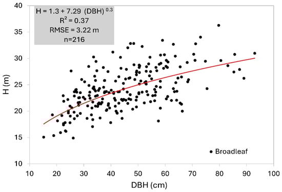
Figure A1.
The H-DBH model for broadleaf species derived from 216 trees in the compartments of 16, 65–66, and 03. Model parameters a and b were 7.29 and 0.3, respectively.
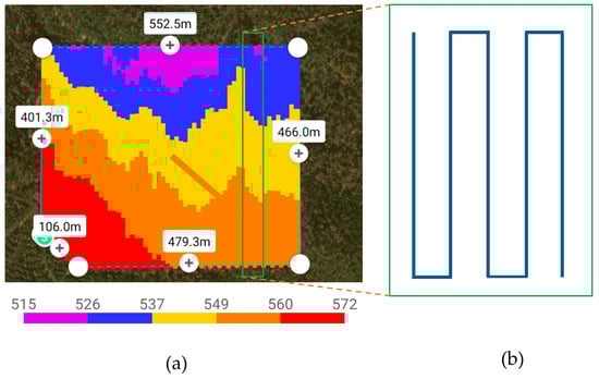
Figure A2.
The flight plan of UAV: (a) flight plan map visible at the controller screen and (b) a zoomed-in portion of flight plan. Elevation of the study area indicated by the legend showing different colors; the plus (+) sign, with a value in m, represents the length of one side of the flight area.
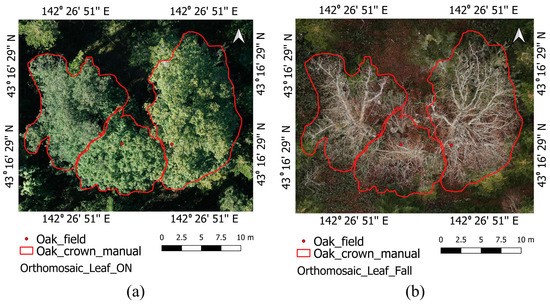
Figure A3.
The manually delineated individual tree crowns (red lines), along with a spatial position of trees (red dots) in a clustered canopy area in RGB orthomosaic: (a) visibility of oak tree crowns in leaf-on seasons (7 October 2023) and (b) visibility of oak tree stem in leaf-fall seasons (8 November 2023).
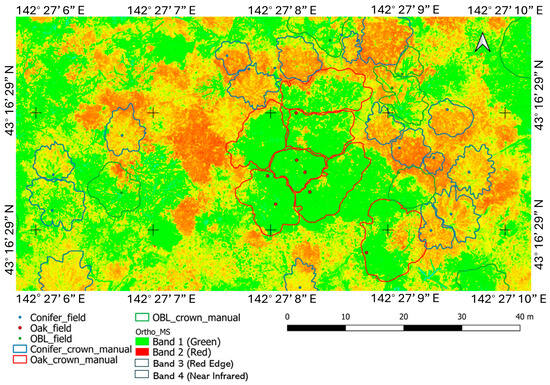
Figure A4.
The individual tree crowns and their geospatial locations for conifer, oak, and OBL in MS orthomosaic. The color distributions in the figure are based on the default settings of Band 1 and Band 2 in QGIS software.
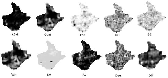
Figure A5.
The visibility of textural metrics of an individual tree crown, e.g., broadleaf species.
References
- Zhou, X.; Zhang, X. Individual Tree Parameters Estimation for Plantation Forests Based on UAV Oblique Photography. IEEE Access 2020, 8, 96184–96198. [Google Scholar] [CrossRef]
- Moe, K.T.; Owari, T. Predicting Individual Tree Growth of High-Value Timber Species in Mixed Conifer-Broadleaf Forests in Northern Japan Using Long-Term Forest Measurement Data. J. For. Res. 2020, 25, 242–249. [Google Scholar] [CrossRef]
- Owari, T.; Okamura, K.; Fukushi, K.; Kasahara, H.; Tatsumi, S. Single-Tree Management for High-Value Timber Species in a Cool-Temperate Mixed Forest in Northern Japan. Int. J. Biodivers. Sci. Ecosyst. Serv. Manag. 2016, 12, 74–82. [Google Scholar] [CrossRef]
- Moe, K.; Owari, T.; Furuya, N.; Hiroshima, T. Comparing Individual Tree Height Information Derived from Field Surveys, LiDAR and UAV-DAP for High-Value Timber Species in Northern Japan. Forests 2020, 11, 223. [Google Scholar] [CrossRef]
- Zhou, Y.; Singh, J.; Butnor, J.R.; Coetsee, C.; Boucher, P.B.; Case, M.F.; Hockridge, E.G.; Davies, A.B.; Staver, A.C. Limited Increases in Savanna Carbon Stocks over Decades of Fire Suppression. Nature 2022, 603, 445–449. [Google Scholar] [CrossRef]
- Bornand, A.; Rehush, N.; Morsdorf, F.; Thürig, E.; Abegg, M. Individual Tree Volume Estimation with Terrestrial Laser Scanning: Evaluating Reconstructive and Allometric Approaches. Agric. For. Meteorol. 2023, 341, 109654. [Google Scholar] [CrossRef]
- Gao, B.; Yu, L.; Ren, L.; Zhan, Z.; Luo, Y. Early Detection of Dendroctonus Valens Infestation at Tree Level with a Hyperspectral UAV Image. Remote Sens. 2023, 15, 407. [Google Scholar] [CrossRef]
- Dobbertin, M. Tree Growth as Indicator of Tree Vitality and of Tree Reaction to Environmental Stress: A Review. Eur. J. For. Res. 2005, 124, 319–333. [Google Scholar] [CrossRef]
- Lausch, A.; Erasmi, S.; King, D.; Magdon, P.; Heurich, M. Understanding Forest Health with Remote Sensing-Part II—A Review of Approaches and Data Models. Remote Sens. 2017, 9, 129. [Google Scholar] [CrossRef]
- Girona, M.M.; Aakala, T.; Aquilué, N.; Bélisle, A.-C.; Chaste, E.; Danneyrolles, V.; Díaz-Yáñez, O.; D’Orangeville, L.; Grosbois, G.; Hester, A.; et al. Challenges for the Sustainable Management of the Boreal Forest Under Climate Change. In Boreal Forests in the Face of Climate Change: Sustainable Management; Springer: Berlin/Heidelberg, Germany, 2023; pp. 773–837. [Google Scholar]
- Zhao, Y.; Im, J.; Zhen, Z.; Zhao, Y. Towards Accurate Individual Tree Parameters Estimation in Dense Forest: Optimized Coarse-to-Fine Algorithms for Registering UAV and Terrestrial LiDAR Data. Gisci. Remote Sens. 2023, 60, 2197281. [Google Scholar] [CrossRef]
- Yun, T.; Jiang, K.; Li, G.; Eichhorn, M.P.; Fan, J.; Liu, F.; Chen, B.; An, F.; Cao, L. Individual Tree Crown Segmentation from Airborne LiDAR Data Using a Novel Gaussian Filter and Energy Function Minimization-Based Approach. Remote Sens. Environ. 2021, 256, 112307. [Google Scholar] [CrossRef]
- Yin, D.; Wang, L. How to Assess the Accuracy of the Individual Tree-Based Forest Inventory Derived from Remotely Sensed Data: A Review. Int. J. Remote. Sens. 2016, 37, 4521–4553. [Google Scholar] [CrossRef]
- Xu, X.; Zhou, Z.; Tang, Y.; Qu, Y. Individual Tree Crown Detection from High Spatial Resolution Imagery Using a Revised Local Maximum Filtering. Remote Sens. Environ. 2021, 258, 112397. [Google Scholar] [CrossRef]
- Liang, X.; Kankare, V.; Hyyppä, J.; Wang, Y.; Kukko, A.; Haggrén, H.; Yu, X.; Kaartinen, H.; Jaakkola, A.; Guan, F.; et al. Terrestrial Laser Scanning in Forest Inventories. ISPRS J. Photogramm. Remote Sens. 2016, 115, 63–77. [Google Scholar] [CrossRef]
- Liu, K.; Shen, X.; Cao, L.; Wang, G.; Cao, F. Estimating Forest Structural Attributes Using UAV-LiDAR Data in Ginkgo Plantations. ISPRS J. Photogramm. Remote Sens. 2018, 146, 465–482. [Google Scholar] [CrossRef]
- Fassnacht, F.E.; White, J.C.; Wulder, M.A.; Næsset, E. Remote Sensing in Forestry: Current Challenges, Considerations and Directions. For. Int. J. For. Res. 2024, 97, 11–37. [Google Scholar] [CrossRef]
- Poley, L.G.; McDermid, G.J. A Systematic Review of the Factors Influencing the Estimation of Vegetation Aboveground Biomass Using Unmanned Aerial Systems. Remote Sens. 2020, 12, 1052. [Google Scholar] [CrossRef]
- Yel, S.G.; Tunc Gormus, E. Exploiting Hyperspectral and Multispectral Images in the Detection of Tree Species: A Review. Front. Remote Sens. 2023, 4, 1136289. [Google Scholar] [CrossRef]
- Wallner, A.; Elatawneh, A.; Schneider, T.; Knoke, T. Estimation of Forest Structural Information Using RapidEye Satellite Data. Forestry 2015, 88, 96–107. [Google Scholar] [CrossRef]
- Morin, D.; Planells, M.; Guyon, D.; Villard, L.; Mermoz, S.; Bouvet, A.; Thevenon, H.; Dejoux, J.-F.; Le Toan, T.; Dedieu, G. Estimation and Mapping of Forest Structure Parameters from Open Access Satellite Images: Development of a Generic Method with a Study Case on Coniferous Plantation. Remote Sens. 2019, 11, 1275. [Google Scholar] [CrossRef]
- Tian, L.; Wu, X.; Tao, Y.; Li, M.; Qian, C.; Liao, L.; Fu, W. Review of Remote Sensing-Based Methods for Forest Aboveground Biomass Estimation: Progress, Challenges, and Prospects. Forests 2023, 14, 1086. [Google Scholar] [CrossRef]
- White, J.C.; Coops, N.C.; Wulder, M.A.; Vastaranta, M.; Hilker, T.; Tompalski, P. Remote Sensing Technologies for Enhancing Forest Inventories: A Review. Can. J. Remote Sens. 2016, 42, 619–641. [Google Scholar] [CrossRef]
- Coops, N.C.; Tompalski, P.; Goodbody, T.R.H.; Queinnec, M.; Luther, J.E.; Bolton, D.K.; White, J.C.; Wulder, M.A.; van Lier, O.R.; Hermosilla, T. Modelling Lidar-Derived Estimates of Forest Attributes over Space and Time: A Review of Approaches and Future Trends. Remote Sens. Environ. 2021, 260, 112477. [Google Scholar] [CrossRef]
- Xu, C.; Morgenroth, J.; Manley, B. Integrating Data from Discrete Return Airborne LiDAR and Optical Sensors to Enhance the Accuracy of Forest Description: A Review. Curr. For. Rep. 2015, 1, 206–219. [Google Scholar] [CrossRef]
- Iglhaut, J.; Cabo, C.; Puliti, S.; Piermattei, L.; O’Connor, J.; Rosette, J. Structure from Motion Photogrammetry in Forestry: A Review. Curr. For. Rep. 2019, 5, 155–168. [Google Scholar] [CrossRef]
- Jayathunga, S.; Owari, T.; Tsuyuki, S. The Use of Fixed–Wing UAV Photogrammetry with LiDAR DTM to Estimate Merchantable Volume and Carbon Stock in Living Biomass over a Mixed Conifer–Broadleaf Forest. Int. J. Appl. Earth Obs. Geoinf. 2018, 73, 767–777. [Google Scholar] [CrossRef]
- Karthigesu, J.; Owari, T.; Tsuyuki, S.; Hiroshima, T. Improving the Estimation of Structural Parameters of a Mixed Conifer–Broadleaf Forest Using Structural, Textural, and Spectral Metrics Derived from Unmanned Aerial Vehicle Red Green Blue (RGB) Imagery. Remote Sens. 2024, 16, 1783. [Google Scholar] [CrossRef]
- Jayathunga, S.; Owari, T.; Tsuyuki, S. Evaluating the Performance of Photogrammetric Products Using Fixed-Wing UAV Imagery over a Mixed Conifer–Broadleaf Forest: Comparison with Airborne Laser Scanning. Remote Sens. 2018, 10, 187. [Google Scholar] [CrossRef]
- Qin, H.; Zhou, W.; Yao, Y.; Wang, W. Individual Tree Segmentation and Tree Species Classification in Subtropical Broadleaf Forests Using UAV-Based LiDAR, Hyperspectral, and Ultrahigh-Resolution RGB Data. Remote Sens. Environ. 2022, 280, 113143. [Google Scholar] [CrossRef]
- Xia, J.; Wang, Y.; Dong, P.; He, S.; Zhao, F.; Luan, G. Object-Oriented Canopy Gap Extraction from UAV Images Based on Edge Enhancement. Remote Sens. 2022, 14, 4762. [Google Scholar] [CrossRef]
- Adão, T.; Hruška, J.; Pádua, L.; Bessa, J.; Peres, E.; Morais, R.; Sousa, J. Hyperspectral Imaging: A Review on UAV-Based Sensors, Data Processing and Applications for Agriculture and Forestry. Remote Sens. 2017, 9, 1110. [Google Scholar] [CrossRef]
- Chai, G.; Zheng, Y.; Lei, L.; Yao, Z.; Chen, M.; Zhang, X. A Novel Solution for Extracting Individual Tree Crown Parameters in High-Density Plantation Considering Inter-Tree Growth Competition Using Terrestrial Close-Range Scanning and Photogrammetry Technology. Comput. Electron. Agric. 2023, 209, 107849. [Google Scholar] [CrossRef]
- Gallardo-Salazar, J.L.; Pompa-García, M. Detecting Individual Tree Attributes and Multispectral Indices Using Unmanned Aerial Vehicles: Applications in a Pine Clonal Orchard. Remote Sens. 2020, 12, 4144. [Google Scholar] [CrossRef]
- Ozdemir, I.; Karnieli, A. Predicting Forest Structural Parameters Using the Image Texture Derived from WorldView-2 Multispectral Imagery in a Dryland Forest, Israel. Int. J. Appl. Earth Obs. Geoinf. 2011, 13, 701–710. [Google Scholar] [CrossRef]
- Ventura, J.; Pawlak, C.; Honsberger, M.; Gonsalves, C.; Rice, J.; Love, N.L.R.; Han, S.; Nguyen, V.; Sugano, K.; Doremus, J.; et al. Individual Tree Detection in Large-Scale Urban Environments Using High-Resolution Multispectral Imagery. Int. J. Appl. Earth Obs. Geoinf. 2024, 130, 103848. [Google Scholar] [CrossRef]
- Sivanandam, P.; Lucieer, A. Tree Detection and Species Classification in a Mixed Species Forest Using Unoccupied Aircraft System (UAS) RGB and Multispectral Imagery. Remote Sens. 2022, 14, 4963. [Google Scholar] [CrossRef]
- Htun, N.M.; Owari, T.; Tsuyuki, S.; Hiroshima, T. Mapping the Distribution of High-Value Broadleaf Tree Crowns through Unmanned Aerial Vehicle Image Analysis Using Deep Learning. Algorithms 2024, 17, 84. [Google Scholar] [CrossRef]
- Silva, C.A.; Hudak, A.T.; Vierling, L.A.; Valbuena, R.; Cardil, A.; Mohan, M.; de Almeida, D.R.A.; Broadbent, E.N.; Almeyda Zambrano, A.M.; Wilkinson, B.; et al. Treetop: A Shiny-based Application and R Package for Extracting Forest Information from LiDAR Data for Ecologists and Conservationists. Methods Ecol. Evol. 2022, 13, 1164–1176. [Google Scholar] [CrossRef]
- Chenge, I.B. Height–Diameter Relationship of Trees in Omo Strict Nature Forest Reserve, Nigeria. Trees For. People 2021, 3, 100051. [Google Scholar] [CrossRef]
- Hulshof, C.M.; Swenson, N.G.; Weiser, M.D. Tree Height-Diameter Allometry across the United States. Ecol. Evol. 2015, 5, 1193–1204. [Google Scholar] [CrossRef]
- Moe, K.T.; Owari, T.; Furuya, N.; Hiroshima, T.; Morimoto, J. Application of UAV Photogrammetry with LiDAR Data to Facilitate the Estimation of Tree Locations and DBH Values for High-Value Timber Species in Northern Japanese Mixed-Wood Forests. Remote Sens. 2020, 12, 2865. [Google Scholar] [CrossRef]
- Stage, A.R. Prediction of Height Increment for Models of Forest Growth; Intermountain Forest and Range Experiment Station, Forest Service, U.S. Department of Agriculture: Ogden, Utah, 1975. [Google Scholar]
- Maezawa, K.; Kawahara, S. A Preparation of the Volume Table for Saghalian Fir (Abies sachalinensis) Trees of the University Forest in Hokkaido. Bull. Tokyo Univ. For. 1985, 74, 17–37. (In Japanese) [Google Scholar]
- Maezawa, K.; Fukushima, Y.; Ichiro, N.; Kawahara, S. A Report on Volume Table for Broad-Leaved Trees of Tokyo University Forest in Hokkaido. Misc. Inf. Univ. Tokyo For. 1968, 17, 77–100. (In Japanese) [Google Scholar]
- Greenhouse Gas Inventory Office of Japan and Ministry of Environment, Japan (Ed.) National Greenhouse Gas Inventory Report of JAPAN 2023; Center for Global Environmental Research, Earth System Division, National Institute for Environmental Studies: Tsukuba, Japan, 2023. [Google Scholar]
- Yang, J.; Zhang, Y.; Du, L.; Liu, X.; Shi, S.; Chen, B. Improving the Selection of Vegetation Index Characteristic Wavelengths by Using the PROSPECT Model for Leaf Water Content Estimation. Remote Sens. 2021, 13, 821. [Google Scholar] [CrossRef]
- Shen, X.; Cao, L.; Yang, B.; Xu, Z.; Wang, G. Estimation of Forest Structural Attributes Using Spectral Indices and Point Clouds from UAS-Based Multispectral and RGB Imageries. Remote Sens. 2019, 11, 800. [Google Scholar] [CrossRef]
- Meng, J.; Li, S.; Wang, W.; Liu, Q.; Xie, S.; Ma, W. Estimation of Forest Structural Diversity Using the Spectral and Textural Information Derived from SPOT-5 Satellite Images. Remote Sens. 2016, 8, 125. [Google Scholar] [CrossRef]
- Ota, T.; Mizoue, N.; Yoshida, S. Influence of Using Texture Information in Remote Sensed Data on the Accuracy of Forest Type Classification at Different Levels of Spatial Resolution. J. For. Res. 2011, 16, 432–437. [Google Scholar] [CrossRef]
- Haralick, R.M.; Shanmugam, K.; Dinstein, I. Textural Features for Image Classification. IEEE Trans. Syst. Man. Cybern. 1973, SMC-3, 610–621. [Google Scholar] [CrossRef]
- Karthigesu, J.; Owari, T.; Tsuyuki, S.; Hiroshima, T. UAV Photogrammetry for Estimating Stand Parameters of an Old Japanese Larch Plantation Using Different Filtering Methods at Two Flight Altitudes. Sensors 2023, 23, 9907. [Google Scholar] [CrossRef]
- Jayathunga, S.; Owari, T.; Tsuyuki, S.; Hirata, Y. Potential of UAV Photogrammetry for Characterization of Forest Canopy Structure in Uneven-Aged Mixed Conifer–Broadleaf Forests. Int. J. Remote. Sens. 2020, 41, 53–73. [Google Scholar] [CrossRef]
- Fraser, R.; Van der Sluijs, J.; Hall, R. Calibrating Satellite-Based Indices of Burn Severity from UAV-Derived Metrics of a Burned Boreal Forest in NWT, Canada. Remote Sens. 2017, 9, 279. [Google Scholar] [CrossRef]
- Richardson, A.J.; Wiegand, C. Distinguishing Vegetation from Soil Background Information. Photogramm. Eng. Remote Sens. 1977, 43, 1541–1552. [Google Scholar]
- Wei, Q.; Li, L.; Ren, T.; Wang, Z.; Wang, S.; Li, X.; Cong, R.; Lu, J. Diagnosing Nitrogen Nutrition Status of Winter Rapeseed via Digital Image Processing Technique. Sci. Agric. Sin. 2020, 48, 3877–3886. [Google Scholar]
- Sellaro, R.; Crepy, M.; Trupkin, S.A.; Karayekov, E.; Buchovsky, A.S.; Rossi, C.; Casal, J.J. Cryptochrome as a Sensor of the Blue/Green Ratio of Natural Radiation in Arabidopsis. Plant. Physiol. 2010, 154, 401–409. [Google Scholar] [CrossRef]
- Kawashima, S.; Nakatani, M. An Algorithm for Estimating Chlorophyll Content in Leaves Using a Video Camera. Ann. Bot. 1998, 81, 49–54. [Google Scholar] [CrossRef]
- Hunt, E.R.; Cavigelli, M.; Daughtry, C.S.T.; Mcmurtrey, J.E.; Walthall, C.L. Evaluation of Digital Photography from Model Aircraft for Remote Sensing of Crop Biomass and Nitrogen Status. Precis. Agric. 2005, 6, 359–378. [Google Scholar] [CrossRef]
- Peñuelas, J.; Gamon, J.A.; Fredeen, A.L.; Merino, J.; Field, C.B. Reflectance Indices Associated with Physiological Changes in Nitrogen- and Water-Limited Sunflower Leaves. Remote Sens. Environ. 1994, 48, 135–146. [Google Scholar] [CrossRef]
- Bendig, J.; Yu, K.; Aasen, H.; Bolten, A.; Bennertz, S.; Broscheit, J.; Gnyp, M.L.; Bareth, G. Combining UAV-Based Plant Height from Crop Surface Models, Visible, and near Infrared Vegetation Indices for Biomass Monitoring in Barley. Int. J. Appl. Earth Obs. Geoinf. 2015, 39, 79–87. [Google Scholar] [CrossRef]
- Xiaoqin, W.; Miaomiao, W.; Shaoqiang, W.; Yundong, W. Extraction of Vegetation Information from Visible Unmanned Aerial Vehicle Images. Trans. CSAE 2015, 31, 152. [Google Scholar]
- Woebbecke, D.M.; Meyer, G.E.; Von Bargen, K.; Mortensen, D.A. Color Indices for Weed Identification under Various Soil, Residue, and Lighting Conditions. Trans. ASAE 1995, 38, 259–269. [Google Scholar] [CrossRef]
- Gitelson, A.A.; Viña, A.; Arkebauer, T.J.; Rundquist, D.C.; Keydan, G.; Leavitt, B. Remote Estimation of Leaf Area Index and Green Leaf Biomass in Maize Canopies. Geophys. Res. Lett. 2003, 30, 1248. [Google Scholar] [CrossRef]
- Belgiu, M.; Drăguţ, L. Random Forest in Remote Sensing: A Review of Applications and Future Directions. ISPRS J. Photogramm. Remote Sens. 2016, 114, 24–31. [Google Scholar] [CrossRef]
- Chai, W.; Saidi, A.; Zine, A.; Droz, C.; You, W.; Ichchou, M. Comparison of Uncertainty Quantification Process Using Statistical and Data Mining Algorithms. Struct. Multidiscip. Optim. 2020, 61, 587–598. [Google Scholar] [CrossRef]
- Krause, S.; Sanders, T.G.M.; Mund, J.-P.; Greve, K. UAV-Based Photogrammetric Tree Height Measurement for Intensive Forest Monitoring. Remote Sens. 2019, 11, 758. [Google Scholar] [CrossRef]
- Jin, X.-L.; Liu, Y.; Yu, X.-B. UAV-RGB-Image-Based Aboveground Biomass Equation for Planted Forest in Semi-Arid Inner Mongolia, China. Ecol. Inform. 2024, 81, 102574. [Google Scholar] [CrossRef]
- Chen, Q.; Gao, T.; Zhu, J.; Wu, F.; Li, X.; Lu, D.; Yu, F. Individual Tree Segmentation and Tree Height Estimation Using Leaf-Off and Leaf-On UAV-LiDAR Data in Dense Deciduous Forests. Remote Sens. 2022, 14, 2787. [Google Scholar] [CrossRef]
- Haralick, R.M. Statistical and Structural Approaches to Texture. Proc. IEEE 1979, 67, 786–804. [Google Scholar] [CrossRef]
- Sripada, R.P.; Heiniger, R.W.; White, J.G.; Weisz, R. Aerial Color Infrared Photography for Determining Late-Season Nitrogen Requirements in Corn. Agron. J. 2005, 97, 1443–1451. [Google Scholar] [CrossRef]
- Moya, I.; Guyot, G.; Goulas, Y. Remotely Sensed Blue and Red Fluorescence Emission for Monitoring Vegetation. ISPRS J. Photogramm. Remote Sens. 1992, 47, 205–231. [Google Scholar] [CrossRef]
- Wu, B.-S.; Mansoori, M.; Schwalb, M.; Islam, S.; Naznin, M.T.; Addo, P.W.; MacPherson, S.; Orsat, V.; Lefsrud, M. Light Emitting Diode Effect of Red, Blue, and Amber Light on Photosynthesis and Plant Growth Parameters. J. Photochem. Photobiol. B 2024, 256, 112939. [Google Scholar] [CrossRef]
- Noguchi, M.; Hoshizaki, K.; Matsushita, M.; Sugiura, D.; Yagihashi, T.; Saitoh, T.; Itabashi, T.; Kazuhide, O.; Shibata, M.; Hoshino, D.; et al. Aboveground Biomass Increments over 26 Years (1993–2019) in an Old-Growth Cool-Temperate Forest in Northern Japan. J. Plant. Res. 2022, 135, 69–79. [Google Scholar] [CrossRef] [PubMed]
- Forrester, D.I. Does Individual-Tree Biomass Growth Increase Continuously with Tree Size? For. Ecol. Manag. 2021, 481, 118717. [Google Scholar] [CrossRef]
- Diószegi, G.; Molnár, V.É.; Nagy, L.A.; Enyedi, P.; Török, P.; Szabó, S. A New Method for Individual Treetop Detection with Low-Resolution Aerial Laser Scanned Data. Model Earth Syst. Environ. 2024, 10, 5225–5240. [Google Scholar] [CrossRef]
- Duncanson, L.I.; Cook, B.D.; Hurtt, G.C.; Dubayah, R.O. An Efficient, Multi-Layered Crown Delineation Algorithm for Mapping Individual Tree Structure across Multiple Ecosystems. Remote Sens. Environ. 2014, 154, 378–386. [Google Scholar] [CrossRef]
- Lu, X.; Guo, Q.; Li, W.; Flanagan, J. A Bottom-up Approach to Segment Individual Deciduous Trees Using Leaf-off Lidar Point Cloud Data. ISPRS J. Photogramm. Remote Sens. 2014, 94, 1–12. [Google Scholar] [CrossRef]
- Jurjević, L.; Liang, X.; Gašparović, M.; Balenović, I. Is Field-Measured Tree Height as Reliable as Believed—Part II, A Comparison Study of Tree Height Estimates from Conventional Field Measurement and Low-Cost Close-Range Remote Sensing in a Deciduous Forest. ISPRS J. Photogramm. Remote Sens. 2020, 169, 227–241. [Google Scholar] [CrossRef]
- Shrestha, R.; Wynne, R.H. Estimating Biophysical Parameters of Individual Trees in an Urban Environment Using Small Footprint Discrete-Return Imaging Lidar. Remote Sens. 2012, 4, 484–508. [Google Scholar] [CrossRef]
- Seidel, D.; Ehbrecht, M.; Puettmann, K. Assessing Different Components of Three-Dimensional Forest Structure with Single-Scan Terrestrial Laser Scanning: A Case Study. For. Ecol. Manag. 2016, 381, 196–208. [Google Scholar] [CrossRef]
- Aalto, I.; Aalto, J.; Hancock, S.; Valkonen, S.; Maeda, E.E. Quantifying the Impact of Management on the Three-Dimensional Structure of Boreal Forests. For. Ecol. Manag. 2023, 535, 120885. [Google Scholar] [CrossRef]
- Zhao, H.; Morgenroth, J.; Pearse, G.; Schindler, J. A Systematic Review of Individual Tree Crown Detection and Delineation with Convolutional Neural Networks (CNN). Curr. For. Rep. 2023, 9, 149–170. [Google Scholar] [CrossRef]
Disclaimer/Publisher’s Note: The statements, opinions and data contained in all publications are solely those of the individual author(s) and contributor(s) and not of MDPI and/or the editor(s). MDPI and/or the editor(s) disclaim responsibility for any injury to people or property resulting from any ideas, methods, instructions or products referred to in the content. |
© 2025 by the authors. Licensee MDPI, Basel, Switzerland. This article is an open access article distributed under the terms and conditions of the Creative Commons Attribution (CC BY) license (https://creativecommons.org/licenses/by/4.0/).