Temporal Autocorrelation of Sentinel-1 SAR Imagery for Detecting Settlement Expansion

Abstract

Urban areas are rapidly expanding globally. The detection of settlement expansion can, however, be challenging due to the rapid rate of expansion, especially for informal settlements. This paper presents a solution in the form of an unsupervised autocorrelation-based approach. Temporal autocorrelation function (ACF) values derived from hyper-temporal Sentinel-1 imagery were calculated for all time lags using VV backscatter values. Various thresholds were applied to these ACF values in order to create urban change maps. Two different orbital combinations were tested over four informal settlement areas in South Africa. Promising results were achieved in the two of the study areas with mean normalized Matthews Correlation Coefficients (MCCn) of 0.79 and 0.78. A lower performance was obtained in the remaining two areas (mean MCCn of 0.61 and 0.65) due to unfavorable building orientations and low building densities. The first results also indicate that the most stable and optimal ACF-based threshold of 95 was achieved when using images from both relative orbits, thereby incorporating more incidence angles. The results demonstrate the capacity of ACF-based methods for detecting settlement expansion. Practically, this ACF-based method could be used to reduce the time and labor costs of detecting and mapping newly built settlements in developing regions.

1. Introduction

Global population distribution in rural and urban areas is being altered by the complex socio-economic process of urbanization. Only 30% of the world’s population lived in urban areas in 1950, which rose to 55% in 2018 [1]. A continued increase is predicted, reaching an estimated 68% in 2050. With more than 90% of the world’s economic activity taking place in urban areas [2], it is understandable that rural–urban migration is so widespread [3]. Despite the economic benefits of urbanization, major problems, such as congestion, air pollution, and food security, arise [4]. Urbanization also leads to land cover and land use changes, amplifying the heat island effect and causing irreversible changes to ecosystems [5]. Research on urban planning, climate change, carbon cycles, and hydrological dynamics therefore requires accurate and timely urban land cover information, preferably at a medium/high spatial resolution [2,6,7].

Traditionally, new settlements are identified by comparing two high-resolution satellite/aerial images captured at different times. However, this process is time- and resource-intensive, and can be negatively affected by human error [8]. Since the rise in remote sensing, urban land cover mapping has predominantly been undertaken using optical imagery [9], captured by moderate to low spatial resolution sensors, such as MODIS and Landsat [10,11]. However, single-source optical imagery has limitations for urban land cover mapping. Two of the main limitations are cloud cover [4,12] and the spectral similarity of urban areas to bare ground [5]. Spectral indices generally result in spectral mixing between built-up are bare areas, resulting in the misclassification of built-up areas as well as changes between these classes, i.e., settlement expansion [13]. Informal settlements, also known as slums, are particularly susceptible to this confusion with bare ground, particularly when imaged using low- or medium-resolution imagery [14].

Due to these limitations, other sources of remote sensing data, such as synthetic aperture radar (SAR), have been increasingly utilized to map urban land cover and urban changes. SAR technology is beneficial due to its cloud penetration capabilities as well as its ability to capture imagery during the night [12]. Building materials generally have strong dielectric properties and distinct geometry and orientation when compared to other land cover types [10,15]. This results in buildings appearing very bright on SAR images relative to other land cover types. Due to these factors, SAR imagery is considered one of the best alternatives or complements to using optical imagery for urban land cover mapping and change detection [5].

In the literature, urban change detection approaches generally fall into one of four categories: algebra-based, statistics-based, transformation-based, and deep learning-based [16]. Algebra-based change detection involves determining changes between two scenes by using pixel-wise algebra, such as differencing, ratioing, or constructing change indices. A change threshold is then usually established, either manually or through a statistical approach, such as Otsu’s method. In [17], the authors achieved kappa values of 0.72 using a normalized difference alpha index for detecting change due to wildfires using polarimetric SAR imagery. Statistics-based approaches employ the statistical distributions of time-series image data in order to detect change [18]. For example, [19] used localized statistical information and density-based clustering in time-series TerraSAR-X imagery to detect urban step change (from-to-change) with F1-scores of 82.72. Transformation-based approaches rely on applying image transformation, such as principal component analysis (PCA), to bi-temporal or multi-temporal image data in order to highlight changes. In [20], the authors made use of PCA and interferometric coherence of ENVISAT ASAR data to detect urban change related to earthquake damage with an overall accuracy of 82.9%. Post-classification change detection is considered a transformation-based approach [16].

While algebra-, statistics-, and transformation-based change detection approaches are fairly well established for urban change detection [21], deep learning approaches for detecting urban change and settlement expansion have become highly popular in the last decade [22]. A variety of neural networks and deep learning architectures have been developed for urban change detection and includes convolutional neural networks (CNN), fully connected networks (FCN), recurrent neural networks (RNN), generative adversarial networks (GAN), deep belief networks (DBN), long short-term memory networks (LSTM), visual image transformers (ViT), autoencoder networks (AE), U-Nets, and Siamese networks. A host of variants, modifications, and combinations of these architectures have also been explored. Deep learning allows the automated extraction of spatial and temporal features required to detect and characterize change [23]. While a complete review of all these architectures and their use in change detection is beyond the scope of this paper, the reader is referred to excellent review papers, such as [16,22,23,24,25]. In [25], the authors point out that CNNs are by far the most commonly used type of deep learning architecture used for change detection in remote sensing, and that SAR imagery is a popular choice of input data. This review is not specific to urban change, however.

Deep learning approaches that focus on SAR and urban change make use of a range of architectures, often in combination, and with various levels of change detection accuracy. In [26], an deep semi-nonnegative matrix factorization (NMF) layer was used to pre-classify an ERS-2 image pair, after which feature extraction and classification was conducted using a singular value decomposition (SVD) network. This network learns nonlinear relationships between images while suppressing noisy unchanged regions and achieved kappa values of 0.9125 over San Francisco. The authors in [27] employed a U-Net on eight ALOS PALSAR pairs for Bangkok. Their model achieved an F1-score of 0.671. In [28], the authors combined U-Net++ (a U-Net variant) with a ViT to extract urban change from Sentinel-1 image pairs over three cities in China. Their F1-scores ranged between 0.9452 and 0.9736. Their model had over 95 million trainable parameters, however, incurring a substantial computational burden to train. In [29], the authors also combined a U-Net with a ViT, but using an ALOS PALSAR-2 image pair of Beijing. Their implementation of depthwise separable convolution reduced the number of parameters in their model and they achieved an F1-score of 0.8614 and a kappa value of 0.7950. In [30], polarimetric L-band UAVSAR imagery of Los Angeles was used to train a weakly supervised stacked AE. Even with very few training pixels, they achieved kappa values of 0.83. In [31], the authors constructed a residual U-Net trained on three Sentinel-1 images of Nanjing, China. They achieved a kappa values of 0.8298 and showed that incorporating residual blocks into the U-Net improved its performance for urban change detection. SAR data are commonly combined with optical imagery for urban change detection, as in [32], who combined Sentinel-1 and Sentinel-2 imagery. A dual-stream U-Net was constructed and trained on the Onera Satellite CD dataset. Their network obtained F1-scores of 0.480 when trained only on Sentinel-1 and an F1-score of 0.600 when trained on the fused SAR/optical dataset. In many of the papers reviewed above, the networks were tested on multiple study areas, and only the highest performance scores are reported here. It is clear, however, that performance depends greatly on the area on which a network was trained or tested. Several authors also pointed out the drawback that supervised deep learning approaches require a substantial number of labelled image datasets in order to train.

Spatial autocorrelation, which is the spatial grouping of similar objects [33], is a well-known concept in the field of remote sensing. Temporal autocorrelation, however, which indicates how an observation is correlated to previous observations [34], is a concept that has not been researched extensively in the remote sensing domain [8]. A few studies have highlighted the efficacy of temporal autocorrelation functions to detect settlement expansion in South Africa, using both optical [8] and SAR [35] imagery. However, these were semi-supervised methods where a significant number of training samples are required for one of the land cover classes, and prior knowledge of the geographical area is crucial.

Recently, an unsupervised method was developed to detect settlement expansion in South Africa using MODIS imagery [36]. However, hyper-temporal SAR imagery is yet to be used in an unsupervised manner to detect settlement expansion. Specifically, the use of a temporal Autocorrelation Function (ACF), as proposed by [35], is yet to be evaluated for settlement expansion using hyper-temporal Sentinel-1 imagery. Sentinel-1 imagery is captured every twelve days in most parts of the world outside of Europe, at a medium spatial resolution, providing valuable information that can be used to improve the detection accuracy of settlement expansion.

This study evaluates the efficacy of using a temporal ACF, derived from hyper-temporal Sentinel-1 imagery, as an unsupervised settlement change detection technique in the Western Cape province of South Africa. The method was applied to imagery from two different Sentinel-1 orbits to determine the impact of the incidence angle on detection accuracy. If successfully developed, this unsupervised method could be used to reduce the time and labor costs of mapping newly built settlements, especially in developing countries.

2. Materials and Methods

2.1. Study Area

Figure 1 shows the four regions in the Western Cape province that were selected. The regions are all informal settlements in or around the city of Cape Town. The Solomon Mahlangu, T3-V5, Endlovini, and Kayamandi settlements are referred to as Site 1, 2, 3, and 4, respectively. The area of each site is 4 km², except Site 3, which has an area of 9 km². These sites were selected due to the evidence of significant settlement expansion post-2016 and due to their varying characteristics, such as building orientation and density, which will test the robustness of the method. Cape Town’s highly variable winter rainfall, which usually peaks in July [37], adds a further challenge as backscatter intensity generally increases with increased soil moisture [38]. The temporal signatures of SAR backscatter are therefore expected to fluctuate as rainfall levels fluctuate.

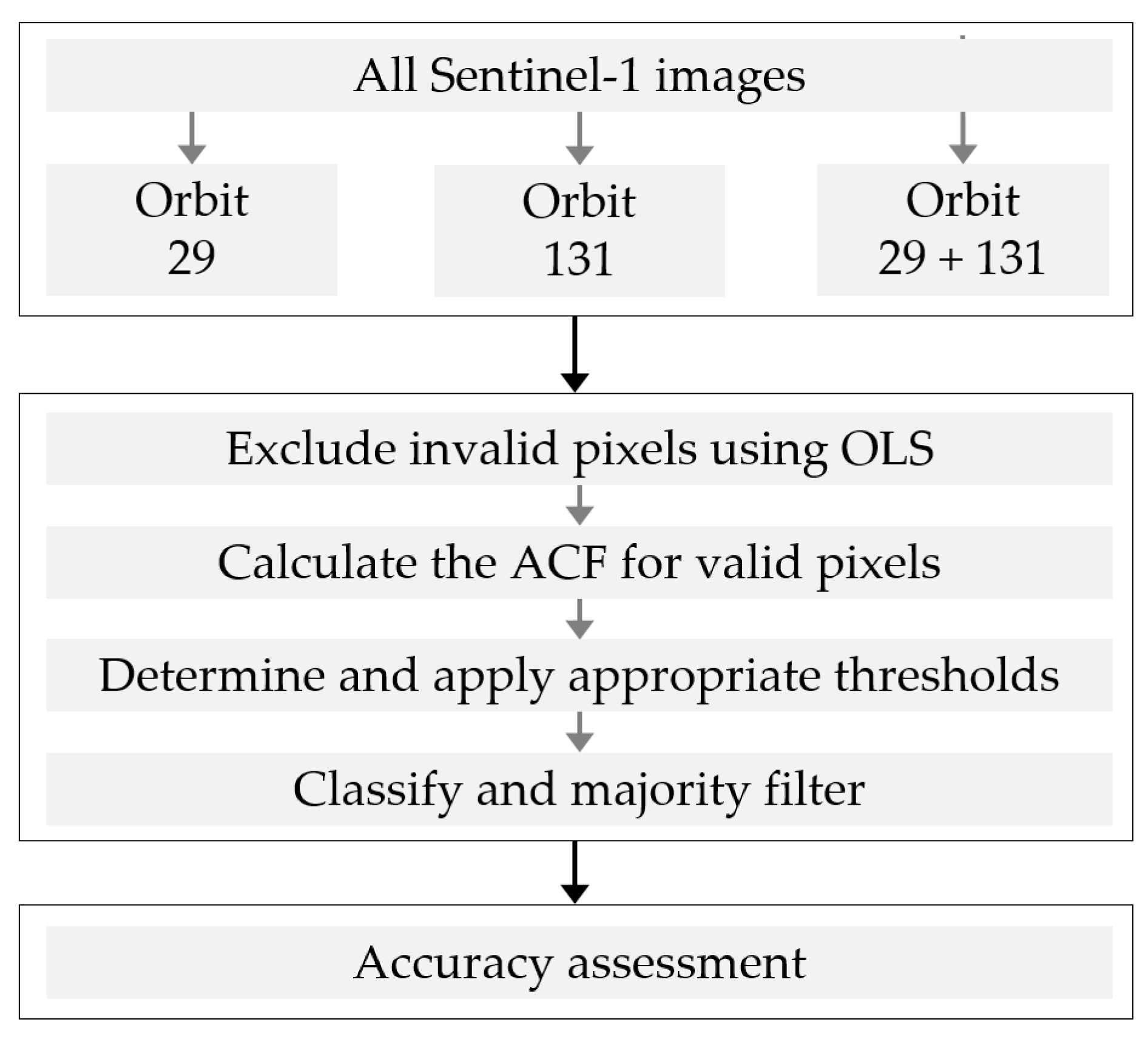
2.2. Experimental Design

The experimental design for the study is shown in Figure 2. The methods employed are described in the following sections and briefly outlined below:

• Acquisition and stacking of Sentinel-1 GRD scenes into three stacks;
• Determination of building orientation;
• Exclusion of invalid pixels;
• Calculation of temporal autocorrelation;
• Thresholding, classification, and filtering of changing pixels;
• Accuracy assessment.

2.3. Data Collection and Preparation

2.3.1. Sentinel-1 Imagery

Google Earth Engine (GEE) was used to access the Sentinel-1 imagery as it is freely available on this cloud-based platform, overcoming data storage and processing limitations [39]. While Sentinel-1 Interferometric Wide imagery is captured in both VV and VH polarizations [40], only the VV polarization was used since co-polarized bands are more sensitive to the surface and double-bounce scattering mechanisms exhibited by buildings [41]. The study area is situated in the overlap zone between two adjacent Sentinel-1 ascending swaths (relative orbits 29 and 131), which allows an investigation of the effect of incidence angle on the analysis. All four areas are covered by the same swath for both orbits 29 and 131, with orbit 131 generally having steeping incidence angles. GEE provides Level-1 Ground Range-Detected (GRD) Sentinel-1 images at a 10 m resampled ground sampling distance. These scenes are radiometrically calibrated sigma-naught (σ°) in decibels (dB) and terrain-corrected using the SRTM 30 m DEM [42].

Table 1. Number of images used for all sites. In 2019, Site 4 had one fewer image available for Orbit 131 as indicated by the numbers in parentheses.

Year	Orbit 29	Orbit 131	Orbit 29 + 131
2016	16	17	33
2017	29	30	59
2018	30	31	61
2019	18	17 (16)	35 (34)
Total	93	95 (94)	188 (187)

summarizes the number of images that were available per year, per orbit for the study sites. An image stack was created per orbit, including a stack with both orbits. These stacks are hereafter referred to as Orbit 29, Orbit 131, and Orbit 29 + 131. Site 4 had one fewer image for Orbit 131 than the other sites in 2019, as indicated in parentheses in Table 1. Each pixel in these stacks contains an array of all the VV values for observations between 1 January 2016 and 31 July 2019.

2.3.2. Google Earth Reference Imagery

High-resolution optical imagery from Google Earth (GE) was used for validation. This imagery was chosen due to the high spatial resolution of the imagery [43] as well as the availability of recently captured imagery. Images before 1 January 2016 were compared visually (i.e., no spectral values were extracted) to images after 31 July 2019 to determine if areas had undergone settlement expansion. GE imagery is, however, known for inconsistent positional accuracies ranging between less than a meter to over eight meters [43,44,45]. This might affect the accuracy metrics employed and is addressed in the “Accuracy assessment” Section (Section 2.8).

2.4. Estimation of Building Orientation

In order to estimate the impact of building orientation on the temporal ACF results, this orientation needed to be determined. The building orientation angle (α) was measured relative to the look direction of the sensor and was estimated from the general orientation of buildings in each area. Due to the marginal difference in the look direction angles of the two relative orbits and the generalized nature of α, the same α value was used for both relative orbits when calculating a polarimetric orientation angle (POA) (θ). POA values ranged from −90° to 90° and were calculated using Equation (1) [46]. For co-polarized bands, double-bounce scattering was maximum when POA was either −90°, 0°, or 90° and was at a minimum when POA was either −45° or 45° [47]. Table 2 shows the building orientation angle, incidence angle (ϕ), and POA for each area per orbit.

$${\mathsf{\theta }=-\tan }^{-1}\left(\frac{\tan \mathsf{\alpha }}{\cos \mathsf{\varphi }}\right)$$

(1)

where θ is the polarimetric orientation angle;

α is the building orientation angle;

ϕ is the sensor incidence angle.

Table 2. Geometry and sensor properties of each area per orbit, along with the calculated POA values. All values in the table are angles measured in degrees (°).

Site	Building Orientation Angle (α)	Orbit 29 (Look Direction = 72°)		Orbit 131 (Look Direction = 73°)
		Incidence Angle (ϕ)	POA (θ)	Incidence Angle (ϕ)	POA (θ)
1	−5	43.23	6.85	32.21	7.11
2	6	43.38	−8.23	32.39	−10.59
3	−37	43.11	45.91	32.05	43.09
4	−28	44.15	36.54	33.33	−57.67
Mean		43.47		32.50

Table 2. Geometry and sensor properties of each area per orbit, along with the calculated POA values. All values in the table are angles measured in degrees (°).

Site	Building Orientation Angle (α)	Orbit 29 (Look Direction = 72°)		Orbit 131 (Look Direction = 73°)
		Incidence Angle (ϕ)	POA (θ)	Incidence Angle (ϕ)	POA (θ)
1	−5	43.23	6.85	32.21	7.11
2	6	43.38	−8.23	32.39	−10.59
3	−37	43.11	45.91	32.05	43.09
4	−28	44.15	36.54	33.33	−57.67
Mean		43.47		32.50

Building densities (relative to the size of a Sentinel-1 pixel) were qualitatively estimated for each area. Although there are many building properties that influence SAR backscatter coefficients [47], only orientation and density were assessed in this study.

2.5. Pixel Exclusion Based on Ordinary Least Squares

Ordinary least squares (OLS) can be used to filter pixels based on the temporal backscatter intensity trend of each pixel.

Table 3. Separation of land cover types according to the OLS slope and intercept.

		Slope
		>1	≤1
Intercept	>−6 dB	Urban (increase)	Urban (stable/decrease)
	≤6 dB	Other to urban	Other (stable/decrease)

shows how this is possible using the slope ($m$) and y-intercept ($b$) of an OLS best-fit line calculated over the VV backscatter intensity ($y$) as a function of time ($x$). Equation (2) was used to calculate $m$ after which $b$ can be calculated using Equation (3).

$$m=\frac{\overline{x}·\overline{y}-\overline{xy}}{{\left(\overline{x}\right)}^2-\overline{x^2}}$$

(2)

$$b=\overline{y}-m\overline{x}$$

(3)

Invalid pixels, in this case, are those that have high y-intercepts or low/negative slopes. These pixels can be ignored as they indicate either an increase in the already existing urban areas (which is generally unlikely but may be present in the data due to speckle and variable rainfall), areas with no change, or areas with decreasing VV, which would indicate a negative change. Therefore, the only pixels that were considered for further analysis were those with a low OLS intercept (<=6 dB) and high OLS slope (>1), represented by the shaded block in Table 3.

These slope and intercept thresholds were chosen using visual inspection and were selected in order to under-filter pixels rather than over-filter them. This filtering is a form of data reduction used to reduce the processing time.

2.6. Autocorrelation Function Calculation

ACF values were calculated for each valid pixel, at every possible time lag, using fast Fourier transform [48] as implemented in the statsmodels python package [49]. ACF values indicate how a time-series correlates with a lagged (previous) version of itself [50]. An ACF value of one indicates a perfect positive correlation, zero indicates no correlation, and negative one indicates a perfect negative correlation. A change in the sign of ACF values when stepping through all the lags can be related to a change in land cover at that specific time lag. The initial positive autocorrelation values followed by a long series of zero or negative values indicate a pixel that no longer correlates with its baseline values and therefore is assumed to have undergone urban expansion. Figure 3 illustrates this concept for an urban expansion pixel (on the left) and a stable pixel (on the right). The ACF values in Figure 3b,d were inverted along the x-axis to show the relationship between ACF values and time, i.e., the VV and ACF graphs share the same x-axis. The consistent pattern of ACF values decreasing to, and staying below, zero as one steps backward through the lags, as shown in Figure 3b, indicates a change indicative of urban expansion. Highly variable ACF values, as shown in Figure 3d, are characteristic of areas that have not undergone change and only experience temporary decorrelation due to factors such as variable rainfall and speckle.

2.7. Thresholding and Classification

The length of the longest sequence of non-positive ACF values was recorded for each valid pixel. Various thresholds were then applied to these lengths to create urban change maps. Upon visual inspection, it was decided that the threshold values from 33 up to and including 62 would be tested for Orbit 29 and Orbit 131, as these images contain VV arrays of similar lengths. A threshold value of 33 means that all pixels with a sequence of non-positive ACF values longer than 33 were classified as urban change. The optimal threshold, which balances errors of omission and commission, should therefore fall within this range. Classified points were converted into a raster image for each threshold using QGIS 2.18, after which a majority filter (two-pixel radius) was applied to remove small clusters of misclassified pixels.

One can reason that the length of non-positive ACF sequences is dependent on the number of images in an image stack. The threshold range was therefore adjusted for Orbit 29 + 131 using Equation (4).

$$T=\frac{t}{n}N$$

(4)

where $T$ is the new threshold;

$t$ is the initial threshold;

$n$ is the initial number of images in the stack;

$N$ is the number of images in the new stack.

Using Equation (4) with $n=95$ resulted in threshold values ranging between 65.31 and 122.69 (rounded to 65 and 123, respectively), and this range was tested in all four sites when using Orbit 29 + 131. After calculating the new threshold range, the same classification and majority filtering techniques were applied to these points as to the ones produced by Orbit 29 and Orbit 131.

2.8. Accuracy Assessment

2.8.1. Sampling Scheme

For validation, samples of change and no change were required. Land cover change is generally a rare event, and the conventional random sampling will not sufficiently represent the change class [51]. A stratified random sampling approach was therefore employed to ensure that sufficient samples were gathered for the change class, as shown in

Table 4. Number of sample points per stratum and area, where md refers to the minimum allowable distance between each point to ensure a spatially representative sample distribution.

Area	Change (Reference) (60%)	Change (Classified) (15%)	No Change (25%)	Total (100%)
Site 3 (3 × 3 km)	144 (md = 60 m)	36 (md = 40 m)	60 (md = 80 m)	240
Sites 1, 2, and 4 (2 × 2 km)	132 (md = 30 m)	33 (md = 20 m)	55 (md = 60 m)	220

. A reference change stratum was created by digitizing large areas of known change, which was determined using GE imagery, as described in Section 2.3.2. The classified change stratum refers to the classification produced by the lowest threshold of Orbit 131 but excludes areas that are already included in the reference change stratum. Areas of no change are those that fall outside both the reference polygon and the classified change raster. Points were then randomly sampled from each stratum, with the following splits: 60% change (reference), 15% change (classified), and 25% no change. To account for spatial autocorrelation, a minimum allowable proximity between sample points was enforced, as shown in Table 4. This minimum distance (md) was chosen relative to the size of the sample areas.

Each sample point was validated using GE imagery. A reference point was marked as change if either the majority of the center pixel changed or if the majority of the pixels in a three-by-three window surrounding the center pixel (i.e., nine pixels) changed. This window approach was adopted to account for the mislabeling of reference points due to GE image offsets.

2.8.2. Accuracy Metrics

As the ACF-based method is designed to distinguish between two classes, a binary confusion matrix was used to quantify correct and incorrect classifications (see

Table 5. Binary confusion matrix.

		Predicted Class		Instances
		P	N
Actual class	P	True Positive (TP)	False Negative (FN)	mp
	N	False Positive (FP)	True Negative (TN)	mn
Estimations		ep	en	m

). Equation (5) was used to quantify the imbalance of a dataset, where an imbalance coefficient $\delta =0$ indicates an equal balance between classes, while values close to 1 or −1 indicate a severe imbalance.

$$\delta =2\frac{m_p}{m}-1$$

(5)

Due to the unsuitability of the Kappa statistic for imbalanced datasets [52], the metrics in

Table 6. Accuracy metrics and their respective biases.

Metric	Abbr.	Equation
Sensitivity	SNS	$\frac{TP}{TP+FN}$
Specificity	SPC	$\frac{TN}{TN+FP}$
Bookmaker Informedness	BM	$SNS+SPC-1$
Matthews Correlation Coefficient	MCC	$\frac{TP·TN-FP·FN}{\sqrt{(TP+FP)(TP+FN)(TN+FP)(TN+FN)}}$
Overall Accuracy	OA	$\frac{TP+TN}{TN+FP+TP+FN}$

were used to quantify the performance of the ACF-based method.

MCC and BM were normalized to the range [0, 1], and these normalized versions are referred to as MCCn and BMn, respectively. Since sensitivity, specificity, BMn, and MCCn values all range between 0 and 1, they can be averaged to produce a mean metric (MM) that can be used to determine the best overall performer. Overall accuracy (OA) was also reported but is not included in the MM as it is biased towards larger classes. MCC is generally a more suitable alternative [53,54].

3. Results

In total, 476 classifications were produced due to the range of thresholds tested for each orbit in each area. The best performing classification (determined using the MM) for each category is displayed in

Table 7. Highest accuracy results for all classifications. The highest result per row is shaded darkly, while the lowest result per row is shaded lightly.

	Site 1 (δ = 0.13)			Site 2 (δ = 0.12)			Site 3 (δ = 0.54)			Site 4 (δ = 0.38)
Orbit	131	29	29 + 131	131	29	29 + 131	131	29	29 + 131	131	29	29 + 131
Threshold	60	45	95	49	47	95	35	44	76	38	41	77
Sensitivity	0.604	0.854	0.802	0.732	0.814	0.825	0.182	0.145	0.145	0.265	0.309	0.279
Specificity	0.911	0.782	0.766	0.821	0.724	0.732	0.914	0.984	0.984	0.901	0.954	0.947
MCCn	0.775	0.816	0.782	0.778	0.767	0.776	0.564	0.630	0.630	0.607	0.682	0.660
BMn	0.758	0.818	0.784	0.777	0.769	0.778	0.548	0.565	0.565	0.583	0.631	0.613
MM	0.762	0.818	0.784	0.777	0.769	0.778	0.552	0.581	0.581	0.589	0.644	0.625
OA	0.777	0.814	0.782	0.782	0.764	0.773	0.746	0.792	0.792	0.705	0.755	0.741

. The highest accuracy (MM = 0.82) was achieved in Site 1 using Orbit 29.

These results indicate that settlement expansion was successfully detected in Sites 1 and 2. However, the detection was less successful in Sites 3 and 4, regardless of the orbit that was used. The imbalance coefficient (δ), calculated using Equation (4), is also displayed for each site, with both Sites 1 and 2 having low positive δ values (indicating balanced classes), while Sites 3 and 4 have higher positive δ values (indicating a larger change class than no-change class). The substantial difference between the sensitivity and specificity values for Sites 3 and 4 is indicative of the class imbalance for the samples at these sites. Nonetheless, particularly low sensitivity values are evident, indicating a general under-classification of urban change areas at these sites.

Figure 4 shows the MCCn values for both orbits (29 and 131) for all sites as a function of the polarimetric orientation angle. There is a clear relationship between the orientation of the urban fabric in the four sites and the performance of the ACF classifier. Classifications with POA values closer to 45° have generally lower accuracy values than those closer to 0 or $\left|-90\right|$.

Choosing an optimal threshold for a binary classification is generally a problem-specific decision with respect to whether higher sensitivity or specificity is preferred. An alternative approach is to combine the classifications for all tested thresholds, thereby producing an occurrence map, as seen in Figure 5. Such occurrence maps were created by concatenating the binary classifications from Orbit 29 for each site such that the values are simply the number of times each pixel has been classified as change over the range of tested thresholds. Higher numbers (lighter colors) indicate a higher probability of change occurring. Figure 5 shows the settlement expansion that occurred in Site 1 (left) and Site 3 (right). Figure 5a,b were captured prior to settlement expansion (10 January 2016), while Figure 5c,d were captured after settlement expansion occurred (10 August 2019). Figure 5e,f shows the occurrence map for the two sites. The imagery shown in this figure is from Google Earth and collected by Maxar Technologies.

Figure 5 confirms that the ACF-based method successfully detected the change in Site 1, but performed poorly in Site 3, with a substantial under-classification of the settlement expansion that has occurred. The results obtained in Site 2 and Site 4 are visually similar to those of Site 1 and Site 3, respectively. The reasons for this variable performance are discussed in the following section.

4. Discussion

4.1. Robustness of ACF-Based Classification

The ACF-based method achieved varying results, as shown in Table 7 and Figure 5. Reasonable accuracies were achieved in Sites 1 and 2, with relatively high MM values ranging between 0.76 and 0.82 for all orbits. High sensitivity values indicate that the method successfully detected settlement expansion in these sites, while high specificity values suggest that false positives are relatively low. Since MCC is a generalized form of Pearson correlation for binary variables [53], it can be interpreted using the same criteria as Pearson’s correlation coefficient (r). The (non-normalized) MCC values of between 0.55 and 0.63 for these areas indicate a moderate performance [55]. However, due to the arbitrary nature of the intervals used to interpret r values [56], these classifications were also qualitatively assessed, as shown in Figure 5. The occurrence map for Site 1, shown in Figure 5, suggests a generally good correlation with ground truth imagery. The mismatch between quantitative and qualitative results could be due to an offset in the GE reference imagery [43,44,45].

Conversely, the ACF-based method performed relatively poorly in Sites 3 and 4. Non-normalized MCC values between 0.12 and 0.36 indicate a negligible correlation for the classifications in these two sites, except in Site 4 when using Orbit 29. Due to the high imbalance of the reference samples in Site 3 (δ = 0.54) and Site 4 (δ = 0.38), the obtained OA values are much higher than the MM, MCCn, and BMn values. The qualitative evaluation of these classifications confirmed poor detection accuracies, as illustrated in Figure 5f, confirming that OA is not a suitable accuracy assessment metric when using imbalanced datasets [53,54]. The results in Site 4 were slightly higher due to a region within the area that was successfully detected.

The incidence angle seems to have a relatively small, but noticeable, impact on the ACF classification results. Generally, a better performance was obtained for Orbit 29, which has a shallower (larger) incidence angle than Orbit 131. The performance gain from using shallower incidence angles was predominantly due to improved sensitivity. This agrees with earlier research that reported that a shallower incidence allows for a better discrimination of urban areas [57,58,59,60]. This is usually due to a combination of higher spatial resolutions achieved at larger incidence angles, as well as the increasing sensitivity to differences in surface roughness that occurs at larger incidence angles [61].

The different orbits also resulted in varying optimal thresholds. If all four sites are considered, Orbit 29 produces the most consistent optimal thresholds (ranging between 41 and 47). Due to the poor detection accuracies in Sites 3 and 4, the optimal thresholds of these sites should be ignored as they are expected to be much lower than in ideal areas. Therefore, when considering only Sites 1 and 2, using both orbits (Orbit 29 + 131) produces the most consistent threshold (both are 95). As these observations are based on only two study sites, the optimal threshold of 95 is a preliminary finding, and further research is required to test its robustness over varying areas. Nevertheless, the availability of more information when using Orbit 29 + 131 does seem to yield more consistent results [47]. Equation (3) appears to have successfully scaled the tested threshold range when using Orbit 29 + 131, indicating that the optimal threshold is strongly related to the size of the image stack being used. This is a promising finding as it ensures the ACF-based method is robust to changes in the image stack size. However, this scaling approach was not tested on smaller image stacks (i.e., fewer than 94 images).

In an operational context, creating and interpreting occurrence maps, such as those in Figure 5, might be more practical. An operator or machine learning algorithm can immediately identify areas that have a high probability of settlement expansion, and hence prioritize the validation of these areas. Using this occurrence map approach could significantly reduce the time required to map settlement expansion and overcome the bias and/or error that can be introduced when selecting an optimal ACF threshold.

4.2. Effect of Building Properties

Building properties, such as alignment, height, density, material, and shape, are known to influence the backscatter value of SAR imagery [12,47]. This in turn affects techniques that use backscatter values to detect buildings.

4.2.1. Building Density

The unsatisfactory results achieved in Sites 3 and 4 are likely due to the low density of settlements in these areas, relative to the size of a Sentinel-1 pixel, as indicated in Figure 6. The received SAR signal of a pixel is the vectorial sum of all the scatterers within that pixel [62,63]. Therefore, the backscatter coefficient of a pixel will be greatly influenced by heterogeneous scatterers, i.e., a mixture of different objects inside one pixel. This is known as the “random walk process” [63] (p. 722) which results in aggregated returns as seen in Figure 6d. The poor results caused by low density settlements is therefore not necessarily a flaw of the method, but rather an inherent limitation caused by the spatial resolution of Sentinel-1 imagery. The ACF-based method should produce more consistent results over areas of different building density if higher resolution imagery is used.

The development dynamics of informal settlements could also affect the method. Informal settlements expand non-linearly and generally experience three stages of growth as defined by [64]:

• Infancy: settlements are built on open land in a dispersed layout, where approximately 50% of the land would be converted into houses;
• Booming: characterized by rapid expansion until most of the vacant land has been converted into settlements. Peaks when approximately 80% of the land has been converted;
• Saturation: characterized by vertical expansion once all the vacant land has been converted.

Due to this non-linear increase in settlement density, it is unlikely that settlements in the phase prior to the booming peak would be detected. This is evident in both Sites 3 and 4, where less than 80% of the vacant land had been converted into settlements and consequently poor accuracies were obtained. This suggests that the ACF-based method, when using Sentinel-1 imagery at least, might only be suitable for detecting settlement expansion towards the end of the booming phase or in the saturation phase of expansion.

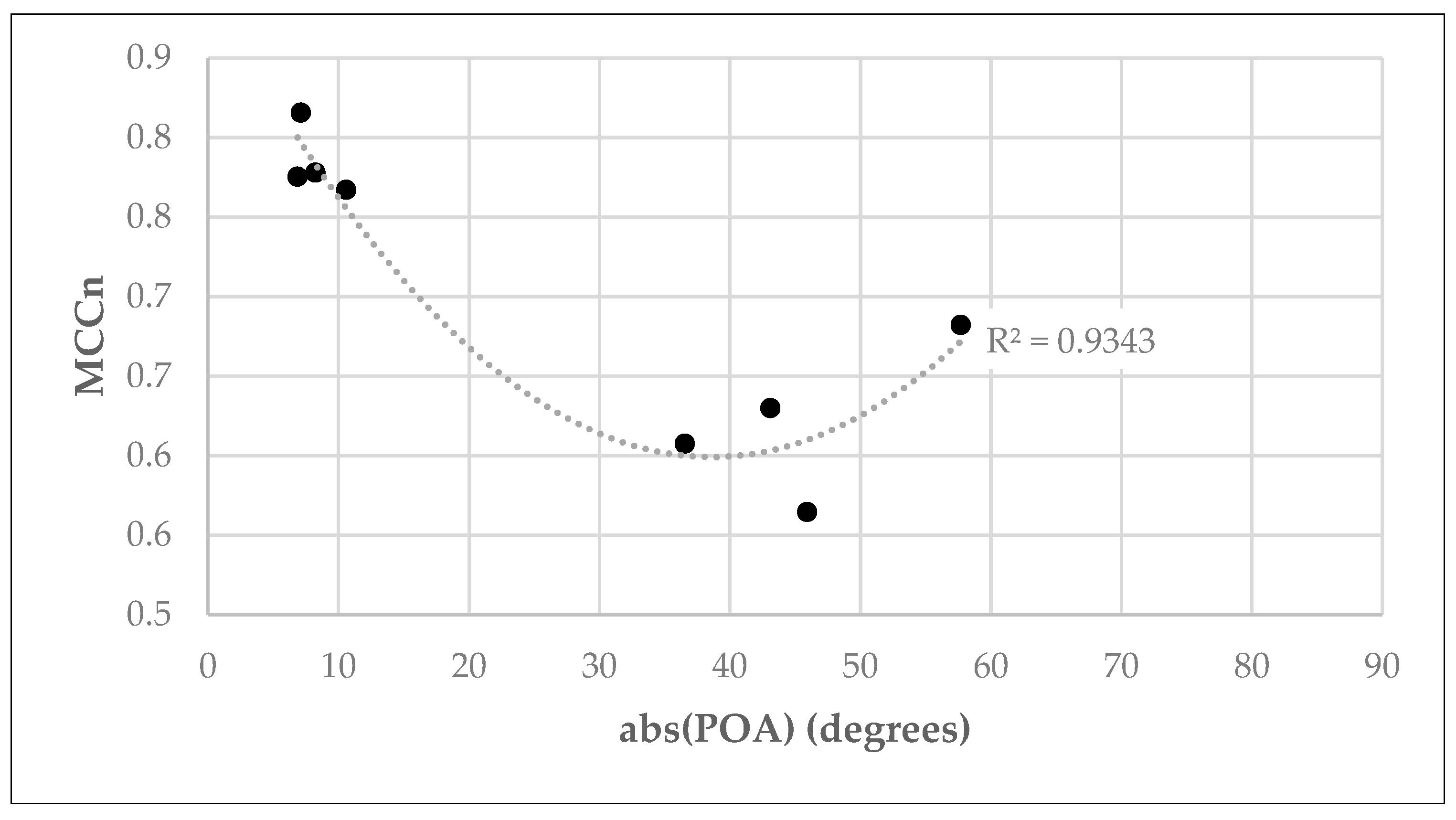
4.2.2. Building Orientation

The orientation of structures is also known to influence the results of urban classifications when using SAR data [65,66]. Ref. [67] found that houses in informal settlements are built to align with existing buildings or infrastructure, such as roads or footpaths. Therefore, even in informal settlements, buildings generally have similar orientations. Due to these similarities, the building orientation angle was generalized over each study site. Evidently, Sites 1 and 2 exhibit almost ideal POAs (close to zero), while Sites 3 and 4 exhibit unfavorable POAs (as seen in Table 2). These values are directly related to the obtained accuracies, as shown in Figure 4, and could therefore explain why settlement expansion was not accurately detected in Sites 3 and 4 [66].

Due to the way building orientation angles were calculated, local variations within each study site were not accounted for. An example of this is found in Site 4, where most of the area is covered by buildings that have an unfavorable orientation in relation to the look direction of the sensor. This is displayed in Figure 7, where the blue line indicates the look direction of the sensor and the red line indicates the orientation of the majority of the buildings in Site 4. However, a small cluster of buildings exhibits a favorable orientation and is therefore detected, as indicated by the yellow region in Figure 7b. The black ellipse in Figure 7b highlights buildings that are densely packed but exhibit unfavorable orientations. These results suggest that orientation has a greater influence on classification performance than density. Site 3 also contains a few regions of high-density buildings, but the majority of these were not detected, further supporting this notion. The use of both ascending and descending passes is therefore recommended when applying the ACF-based method.

Density and orientation are, however, only two of the structural properties that influence SAR urban mapping. In [47], the authors investigated how Sentinel-1 backscatter is influenced by the alignment, height, density, material, and shape of buildings. Their results indicate that building height has the greatest effect on backscatter, density has a moderate effect, and orientation has the lowest effect. They do, however, concede that many of these properties are interrelated and therefore their individual effects cannot be completely quantified. To mitigate the issues caused by variable building properties, the authors suggest that a combination of the co-polarized (VV) and cross-polarized (VH) Sentinel-1 bands be used for urban mapping. They found that using this combination significantly improved detection effectiveness, compared to using VV and VH individually.

4.3. Comparison to Other Methods

When compared to supervised urban change detection methods [2,6,68], the ACF-based method produced inferior results. This is to be expected due to the unsupervised nature of this method. Various unsupervised methods have been developed using SAR imagery. Model-based polarimetric decomposition was implemented by [69] to map urban areas. In particular, their method successfully detected buildings with unfavorable orientations (kappa = 0.845), thereby overcoming one of the limitations of the ACF-based method. The authors in [70] developed a method that selects automatic thresholds for urban change detection mapping, achieving sensitivity values of 0.81 in Toronto and 0.85 in Beijing. Our ACF-based method produced comparable sensitivity values of 0.85 in Site 1 and 0.82 in Site 2. Recently, [71] developed an unsupervised change detection method (not exclusively for urban detection) using a deep fusion network. Their method exhibited low processing time and high accuracies exceeding 90%. Incorporating more polarimetric decomposition parameters in the ACF-based method, rather than relying only on backscatter, is expected to result in an increased change detection performance. Compared specifically to deep learning approaches, such as [28,29,72], our ACF-based method generally under-performed. Similar to many of the deep learning studies, however, our performance depended on the area. Our approach produced comparable or even superior results to some deep learning studies, such as [27,32], without the need for training data.

ACF-based techniques, such as those developed by [8,35,73], were shown to effectively detect urban expansion at a regional scale. Specifically, when using ENVISAT ASAR imagery, the semi-supervised ACF method developed by [35] achieved an overall accuracy of 93%. The difference between the ACF-based method in this paper and that of [35] is that they summed ACF values of the first 23 time lags (the optimal value determined by [74]), while the method developed in this paper counts the longest sequence of non-positive ACF values using all possible time lags. To the best of the authors’ knowledge, this use of ACF values has not been implemented before. This research adds to the body of knowledge concerning the efficacy of using ACF-based methods for remote sensing applications.

4.4. Limitations and Future Recommendations

As mentioned in Section 4.1, testing the effect of incidence angle on this method would require the testing of a greater number and spatial distribution of study sites. Section 4.2 highlights the limitation of the ACF-based method with regards to the orientation and density of settlements. Further research is required to determine which of these factors has a greater influence on the effectiveness of the method and to investigate possible solutions.

The pre-filtering of invalid pixels using ordinary least squares employed in this study was aimed at reducing processing requirements. The effect of this process was not investigated or tested, and therefore further research should be undertaken to either validate or invalidate the usefulness of OLS pre-filtering. However, this filtering did significantly reduce the number of pixels required for further processing, in some cases up to 80%.

The Google Colaboratory cloud-based python environment was used for image acquisition (via Google Earth Engine), OLS pre-filtering, and calculation of ACF values. This environment has various advantages but is not suitable for the operational implementation of the ACF-based method due to runtime restrictions. Converting the existing code into a local Python environment could overcome this limitation. Regardless of the environment, processing time is an issue hindering operational implementation. Currently, the processing time of each pixel is approximately two seconds, which is slow considering the number of pixels in a single Sentinel-1 scene. While the process remains unsupervised and does not require a training period, more efficient methods of processing should be investigated before this method becomes operationally viable.

Speckle negatively affects most techniques that use SAR imagery [63]. In [35], the authors pointed out that their ACF change detection method is not influenced by speckle as local variations in the time-series will not affect the overall trend of the data. However, with the ACF-based method in this paper, local variations could interrupt the sequence of non-positive ACF values. Speckle filtering is therefore expected to improve the effectiveness of the method.

This ACF-based method shows promise, not only for mapping settlement expansion detection, but also for the estimation of the time at which the expansion took place. The relationship between ACF values and the increase in VV backscatter coefficient is evident in Figure 3. This paper highlighted the potential of using ACF values for detecting settlement expansion. However, the effectiveness of using ACF time lags to determine the time of settlement expansion was not investigated. Future research regarding the use of ACF for remote sensing applications could focus on this aspect.

5. Conclusions

Although settlement expansion is a commonly occurring process [8], detection thereof can be challenging. This is partly due to the rapid rate at which settlements—especially informal settlements—are established. In this paper, a possible solution to this problem was presented in the form of an unsupervised ACF-based approach. The efficacy of applying a threshold to calculated ACF values was evaluated. ACF values were calculated for all possible time lags using co-polarized (VV) backscatter coefficient values. Three different orbital combinations were tested (29, 131, and 29 + 131) over four study sites.

The ACF-based method successfully mapped the settlement expansion in Sites 1 and 2 (mean MCCn of 0.79 and 0.78, respectively) but performed poorly in Sites 3 and 4 (mean MCCn of 0.61 and 0.65, respectively). This variable performance is possibly due to the differences in building orientations and densities between these areas. The results also indicate an improvement when using the shallower incidence angle (Orbit 29). However, using both orbits (Orbit 29 + 131) results in a more consistent ACF threshold value of 95, for both Sites 1 and 2. It was also found that the obtained threshold value is strongly related to the size of the image stack that is being processed. As the optimal threshold value is inconclusive, an alternative would be to use an occurrence map approach that spatially indicates the probability of settlement expansion within an area.

The results obtained in this research indicate that ACF is capable of detecting and mapping settlement expansion. The value of the ACF approach lies in its unsupervised nature, which requires no training data. This makes the method more efficient than supervised change detection approaches that require large training datasets to be collected and algorithms to be trained. The method also shows promise with regards to detecting the specific time at which settlement expansion took place, and more research is required to develop the efficacy of this approach.

References

1. United Nations Department of Economic and Social Affairs (Population Division). World Urbanization Prospects 2018: Highlights (ST/ESA/SER.A/421); United Nations Department of Economic and Social Affairs: New York, NY, USA, 2019. [Google Scholar]
2. Li, X.; Gong, P.; Liang, L. A 30-Year (1984–2013) Record of Annual Urban Dynamics of Beijing City Derived from Landsat Data. Remote Sens. Environ. 2015, 166, 78–90. [Google Scholar] [CrossRef]
3. Lopez, J.F.; Shimoni, M.; Grippa, T. Extraction of African Urban and Rural Structural Features Using SAR Sentinel-1 Data. In Proceedings of the 2017 Joint Urban Remote Sensing Event (JURSE), Dubai, United Arab Emirates, 6–8 March 2017; IEEE: Piscataway, NJ, USA, 2017; pp. 1–4. [Google Scholar]
4. Zhou, T.; Li, Z.; Pan, J. Multi-Feature Classification of Multi-Sensor Satellite Imagery Based on Dual-Polarimetric Sentinel-1A, Landsat-8 OLI, and Hyperion Images for Urban Land-Cover Classification. Sensors 2018, 18, 373. [Google Scholar] [CrossRef]
5. Sinha, S.; Santra, A.; Mitra, S.S. A Method for Built-up Area Extraction Using Dual Polarimetric ALOS PALSAR. ISPRS Ann. Photogramm. Remote Sens. Spat. Inf. Sci. 2018, 4, 455–458. [Google Scholar] [CrossRef]
6. Gong, P.; Li, X.; Zhang, W. 40-Year (1978—2017) Human Settlement Changes in China Reflected by Impervious Surfaces from Satellite Remote Sensing. Sci. Bull. 2019, 64, 756–763. [Google Scholar] [CrossRef] [PubMed]
7. Liu, X.; Hu, G.; Chen, Y.; Li, X.; Xu, X.; Li, S.; Pei, F.; Wang, S. High-Resolution Multi-Temporal Mapping of Global Urban Land Using Landsat Images Based on the Google Earth Engine Platform. Remote Sens. Environ. 2018, 209, 227–239. [Google Scholar] [CrossRef]
8. Kleynhans, W.; Salmon, B.P.; Olivier, J.C.; van den Bergh, F.; Wessels, K.J.; Grobler, T.L.; Steenkamp, K.C. Land Cover Change Detection Using Autocorrelation Analysis on MODIS Time-Series Data: Detection of New Human Settlements in the Gauteng Province of South Africa. IEEE J. Sel. Top. Appl. Earth Obs. Remote Sens. 2012, 5, 777–783. [Google Scholar] [CrossRef]
9. Ratha, D.; Gamba, P.; Bhattacharya, A.; Frery, A.C. Novel Techniques for Built-up Area Extraction from Polarimetric SAR Images. IEEE Geosci. Remote Sens. Lett. 2019, 17, 177–181. [Google Scholar] [CrossRef]
10. Sun, Z.; Xu, R.; Du, W.; Wang, L.; Lu, D. High-Resolution Urban Land Mapping in China from Sentinel 1A/2 Imagery Based on Google Earth Engine. Remote Sens. 2019, 11, 752. [Google Scholar] [CrossRef]
11. Callaghan, K.; Engelbrecht, J.; Kemp, J. The Use of Landsat and Aerial Photography for the Assessment of Coastal Erosion and Erosion Susceptibility in False Bay, South Africa. S. Afr. J. Geomat. 2015, 4, 65–79. [Google Scholar] [CrossRef]
12. Zhou, T.; Zhao, M.; Sun, C.; Pan, J. Exploring the Impact of Seasonality on Urban Land-Cover Mapping Using Multi-Season Sentinel-1A and GF-1 WFV Images in a Subtropical Monsoon-Climate Region. ISPRS Int. J. Geoinf. 2017, 7, 3. [Google Scholar] [CrossRef]
13. Dolean, B.E.; Bilașco, Ș.; Petrea, D.; Moldovan, C.; Vescan, I.; Roșca, S.; Fodorean, I. Evaluation of the Built-Up Area Dynamics in the First Ring of Cluj-Napoca Metropolitan Area, Romania by Semi-Automatic GIS Analysis of Landsat Satellite Images. Appl. Sci. 2020, 10, 7722. [Google Scholar] [CrossRef]
14. Weng, Q. Remote Sensing of Impervious Surfaces in the Urban Areas: Requirements, Methods, and Trends. Remote Sens. Environ. 2012, 117, 34–49. [Google Scholar] [CrossRef]
15. Chini, M.; Pelich, R.; Hostache, R.; Matgen, P.; Lopez-martinez, C. Polarimetric and Multitemporal Information Extracted from Sentinel-1 SAR Data to Map Buildings. In Proceedings of the International Geoscience and Remote Sensing Symposium (IGARSS), Kuala Lumpur, Malaysia, 17–22 July 2022; IEEE: Piscataway, NJ, USA, 2018; pp. 8688–8690. [Google Scholar]
16. Parelius, E.J. A Review of Deep-Learning Methods for Change Detection in Multispectral Remote Sensing Images. Remote Sens. 2023, 15, 2092. [Google Scholar] [CrossRef]
17. Engelbrecht, J.; Theron, A.; Vhengani, L.; Kemp, J. A Simple Normalized Difference Approach to Burnt Area Mapping Using Multi-Polarisation C-Band SAR. Remote Sens. 2017, 9, 764. [Google Scholar] [CrossRef]
18. Vu, P.X.; Duc, N.T.; Yem, V.V. Application of Statistical Models for Change Detection in SAR Imagery. In Proceedings of the 2015 International Conference on Computing, Management and Telecommunications (ComManTel), DaNang, Vietnam, 28–30 December 2015; pp. 239–244. [Google Scholar] [CrossRef]
19. Yuan, J.; Lv, X.; Dou, F.; Yao, J. Change Analysis in Urban Areas Based on Statistical Features and Temporal Clustering Using TerraSAR-X Time-Series Images. Remote Sens. 2019, 11, 926. [Google Scholar] [CrossRef]
20. Li, Q.; Gong, L.; Zhang, J. A Correlation Change Detection Method Integrating PCA and Multi- Texture Features of SAR Image for Building Damage Detection. Eur. J. Remote Sens. 2019, 52, 435–447. [Google Scholar] [CrossRef]
21. Jensen, J.R.; Im, J. Remote Sensing Change Detection in Urban Environments. In Geo-Spatial Technologies in Urban Environments (Second Edition): Policy, Practice, and Pixels; Springer: Berlin/Heidelberg, Germany, 2007; pp. 7–31. [Google Scholar]
22. Shafique, A.; Cao, G.; Khan, Z.; Asad, M.; Aslam, M. Deep Learning-Based Change Detection in Remote Sensing Images: A Review. Remote Sens. 2022, 14, 871. [Google Scholar] [CrossRef]
23. Bai, T.; Wang, L.; Yin, D.; Sun, K.; Chen, Y.; Li, W.; Li, D. Deep Learning for Change Detection in Remote Sensing: A Review. Geo-Spat. Inf. Sci. 2022, 1–27. [Google Scholar] [CrossRef]
24. Shi, W.; Zhang, M.; Zhang, R.; Chen, S.; Zhan, Z. Change Detection Based on Artificial Intelligence: State-of-the-Art and Challenges. Remote Sens. 2020, 12, 1688. [Google Scholar] [CrossRef]
25. Khelifi, L.; Mignotte, M. Deep Learning for Change Detection in Remote Sensing Images: Comprehensive Review and Meta-Analysis. IEEE Access 2020, 8, 126385–126400. [Google Scholar] [CrossRef]
26. Gao, F.; Liu, X.; Dong, J.; Zhong, G.; Jian, M. Change Detection in SAR Images Based on Deep Semi-NMF and SVD Networks. Remote Sens. 2017, 9, 435. [Google Scholar] [CrossRef]
27. Jaturapitpornchai, R.; Matsuoka, M.; Kanemoto, N.; Kuzuoka, S.; Ito, R.; Nakamura, R. Sar-Image Based Urban Change Detection in Bangkok, Thailand Using Deep Learning. In Proceedings of the International Geoscience and Remote Sensing Symposium (IGARSS), Yokohama, Japan, 28 July–2 August 2019; pp. 7403–7406. [Google Scholar] [CrossRef]
28. Du, Y.; Zhong, R.; Li, Q.; Zhang, F. TransUNet++SAR: Change Detection with Deep Learning about Architectural Ensemble in SAR Images. Remote Sens. 2022, 15, 6. [Google Scholar] [CrossRef]
29. Pang, L.; Sun, J.; Chi, Y.; Yang, Y.; Zhang, F.; Zhang, L. CD-TransUNet: A Hybrid Transformer Network for the Change Detection of Urban Buildings Using L-Band SAR Images. Sustainability 2022, 14, 9847. [Google Scholar] [CrossRef]
30. De, S.; Pirrone, D.; Bovolo, F.; Bruzzone, L.; Bhattacharya, A. A Novel Change Detection Framework Based on Deep Learning for the Analysis of Multi-Temporal Polarimetric SAR Images. In Proceedings of the International Geoscience and Remote Sensing Symposium (IGARSS), Fort Worth, TX, USA, 23–28 July 2017; pp. 5193–5196. [Google Scholar] [CrossRef]
31. Li, L.; Wang, C.; Zhang, H.; Zhang, B. Residual Unet for Urban Building Change Detection with Sentinel-1 SAR Data. In Proceedings of the International Geoscience and Remote Sensing Symposium (IGARSS), Yokohama, Japan, 28 July–2 August 2019; pp. 1498–1501. [Google Scholar] [CrossRef]
32. Hafner, S.; Nascetti, A.; Azizpour, H.; Ban, Y. Sentinel-1 and Sentinel-2 Data Fusion for Urban Change Detection Using a Dual Stream U-Net. IEEE Geosci. Remote Sens. Lett. 2022, 19, 1–5. [Google Scholar] [CrossRef]
33. Brown, T.T.; Wood, J.D.; Griffith, D.A. Using Spatial Autocorrelation Analysis to Guide Mixed Methods Survey Sample Design Decisions. J. Mix. Methods Res. 2017, 11, 394–414. [Google Scholar] [CrossRef]
34. Madsen, H. Time Series Analysis; Chapman and Hall/CRC: Boca Raton, FL, USA, 2007. [Google Scholar]
35. Kleynhans, W.; Salmon, B.P.; Wessels, K.J.; Olivier, J.C. Rapid Detection of New and Expanding Human Settlements in the Limpopo Province of South Africa Using a Spatio-Temporal Change Detection Method. Int. J. Appl. Earth Obs. Geoinf. 2015, 40, 74–80. [Google Scholar] [CrossRef]
36. Olding, W.C.; Olivier, J.C.; Salmon, B.P.; Kleynhans, W. Unsupervised Land Cover Change Estimation Using Region Covariance Estimates. IEEE Geosci. Remote Sens. Lett. 2019, 16, 347–351. [Google Scholar] [CrossRef]
37. Mahlalela, P.T.; Blamey, R.C.; Cjc, R. Mechanisms behind Early Winter Rainfall Variability in the Southwestern Cape, South Africa. Clim. Dyn. 2019, 53, 21–39. [Google Scholar] [CrossRef]
38. Ulaby, F.T.; Dubois, P.C.; Van Zyl, J. Radar Mapping of Surface Soil Moisture. J. Hydrol. 1996, 184, 57–84. [Google Scholar] [CrossRef]
39. Gorelick, N.; Hancher, M.; Dixon, M.; Ilyushchenko, S.; Thau, D.; Moore, R. Google Earth Engine: Planetary-Scale Geospatial Analysis for Everyone. Remote Sens. Environ. 2017, 202, 18–27. [Google Scholar] [CrossRef]
40. Torres, R.; Snoeij, P.; Geudtner, D.; Bibby, D.; Davidson, M.; Attema, E.; Potin, P.; Rommen, B.; Floury, N.; Brown, M.; et al. GMES Sentinel-1 Mission. Remote Sens. Environ. 2012, 120, 9–24. [Google Scholar] [CrossRef]
41. Chu, H.; Ge, L.; Wang, X. Using Dual-Polarised L-Band SAR and Optical Satellite Imagery for Land Cover Classification in Southern Vietnam: Comparison and Combination. In Proceedings of the 10th Australian Space Science Conference Series, Brisbane, Australia, 27–30 September 2010. [Google Scholar]
42. Google. Sentinel-1 Algorithms. Available online: https://developers.google.com/earth-engine/guides/sentinel1 (accessed on 12 August 2023).
43. Goudarzi, M.A.; Landry, R.J. Assessing Horizontal Positional Accuracy of Google Earth Imagery in the City of Montreal, Canada. Geod. Cartogr. 2017, 43, 56–65. [Google Scholar] [CrossRef]
44. Pulighe, G.; Baiocchi, V.; Lupia, F. Horizontal Accuracy Assessment of Very High Resolution Google Earth Images in the City of Rome, Italy. Int. J. Digit. Earth 2016, 9, 342–362. [Google Scholar] [CrossRef]
45. Ubukawa, T. An Evaluation of the Horizontal Positional Accuracy of Google and Bing Satellite Imagery and Three Roads Data Sets Based on High Resolution Satellite Imagery; Center for International Earth Science Information Network (CIESIN): Palisades, NY, USA, 2013. [Google Scholar]
46. Kimura, H. Radar Polarization Orientation Shifts in Built-up Areas. IEEE Geosci. Remote Sens. Lett. 2008, 5, 217–221. [Google Scholar] [CrossRef]
47. Koppel, K.; Zalite, K.; Voormansik, K.; Jagdhuber, T. Sensitivity of Sentinel-1 Backscatter to Characteristics of Buildings. Int. J. Remote Sens. 2017, 38, 6298–6318. [Google Scholar] [CrossRef]
48. Robertson, C.; George, S.C. Theory and Practical Recommendations for Autocorrelation-Based Image Correlation Spectroscopy. J. Biomed. Opt. 2012, 17, 80801. [Google Scholar] [CrossRef] [PubMed]
49. McKinney, W.; Perktold, J.; Seabold, S. Time Series Analysis in Python with Statsmodels. In Proceedings of the 10th Python in Science Conference (SCIPY 2011), Austin, TX, USA, 11–16 July 2011; pp. 96–102. [Google Scholar]
50. Tinungki, G.M. The Analysis of Partial Autocorrelation Function in Predicting Maximum Wind Speed. In Proceedings of the IOP Conference Series: Earth and Environmental Science, Makassar, Indonesia, 30 August–1 September 2018; IOP Publishing: Bristol, UK, 2019; p. 12097. [Google Scholar]
51. Congalton, R.G.; Green, K. Assessing the Accuracy of Remotely Sensed Data: Principles and Practices, 2nd ed.; Taylor & Francis: Oxford, UK, 2019. [Google Scholar]
52. Allouche, O.; Tsoar, A.; Kadmon, R. Assessing the Accuracy of Species Distribution Models: Prevalence, Kappa and the True Skill Statistic (TSS). J. Appl. Ecol. 2006, 43, 1223–1232. [Google Scholar] [CrossRef]
53. Boughorbel, S.; Jarray, F.; El-Anbari, M. Optimal Classifier for Imbalanced Data Using Matthews Correlation Coefficient Metric. PLoS ONE 2017, 12, e0177678. [Google Scholar] [CrossRef]
54. Luque, A.; Carrasco, A.; Martín, A.; de las Heras, A. The Impact of Class Imbalance in Classification Performance Metrics Based on the Binary Confusion Matrix. Pattern Recognit. 2019, 91, 216–231. [Google Scholar] [CrossRef]
55. Mukaka, M.M. Statistics Corner: A Guide to Appropriate Use of Correlation Coefficient in Medical Research. Malawi Med. J. 2012, 24, 69–71. [Google Scholar]
56. Schober, P.; Schwarte, L.A. Correlation Coefficients: Appropriate Use and Interpretation. Anesth. Analg. 2018, 126, 1763–1768. [Google Scholar] [CrossRef] [PubMed]
57. Corbane, C.; Baghdadi, N.; Descombes, X.; Junior, G.W.; Villeneuve, N.; Petit, M. Comparative Study on the Performance of Multiparameter Sar Data for Operational Urban Areas Extraction Using Textural Features. IEEE Geosci. Remote Sens. Lett. 2009, 6, 728–732. [Google Scholar] [CrossRef]
58. Xia, Z.G.; Henderson, F.M. Understanding the Relationships between Radar Response Patterns and the Bio- and Geophysical Parameters of Urban Areas. IEEE Trans. Geosci. Remote Sens. 1997, 35, 93–101. [Google Scholar] [CrossRef]
59. Henderson, F.M. An Analysis of Settlement Characterization in Central Europe Using SIR-B Radar Imagery. Remote Sens. Environ. 1995, 54, 61–70. [Google Scholar] [CrossRef]
60. Sunuprapto, H.; Hussin, Y.A. A Comparison Between Optical and Radar Satellite Images in Detecting Burnt Tropical Forest in South Sumatra, Indonesia. Int. Arch. Photogramm. Remote Sens. 2000, XXXIII, 580–587. [Google Scholar]
61. Ulaby, F.T.; Fawwaz, T.; Dobson, M.C.; Álvarez-Pérez, J.L. Handbook of Radar Scattering Statistics for Terrain; Artech House: London, UK, 2019; ISBN 1630817023. [Google Scholar]
62. Sen, L.J. Speckle Analysis and Smoothing of Synthetic Aperture Radar Images. Comput. Graph. Image Process. 1981, 17, 24–32. [Google Scholar]
63. Xie, H.; Pierce, L.E.; Ulaby, F.T. Statistical Properties of Logarithmically Transformed Speckle. IEEE Trans. Geosci. Remote Sens. 2002, 40, 721–727. [Google Scholar] [CrossRef]
64. Abebe, F.K. Modelling Informal Settlement Growth in Dar Es Salaam, Tanzania. Master’s Thesis, University of Twente, Enskord, The Netherlands, 2011. [Google Scholar]
65. Ferro, A.; Brunner, D.; Bruzzone, L.; Lemoine, G. On the Relationship between Double Bounce and the Orientation of Buildings in VHR SAR Images. IEEE Geosci. Remote Sens. Lett. 2011, 8, 612–616. [Google Scholar] [CrossRef]
66. Li, H.; Li, Q.; Wu, G.; Chen, J.; Liang, S. The Impacts of Building Orientation on Polarimetric Orientation Angle Estimation and Model-Based Decomposition for Multilook Polarimetric SAR Data in Urban Areas. IEEE Trans. Geosci. Remote Sens. 2016, 54, 5520–5532. [Google Scholar] [CrossRef]
67. Augustijn-Beckers, E.W.; Flacke, J.; Retsios, B. Simulating Informal Settlement Growth in Dar Es Salaam, Tanzania: An Agent-Based Housing Model. Comput. Environ. Urban Syst. 2011, 35, 93–103. [Google Scholar] [CrossRef]
68. Celik, N. Change Detection of Urban Areas in Ankara through Google Earth Engine. In Proceedings of the 41st International Conference on Telecommunications and Signal Processing, Athens, Greece, 4–6 July 2018; IEEE: Piscataway, NJ, USA, 2018; pp. 1–5. [Google Scholar]
69. Xiang, D.; Tang, T.; Ban, Y.; Su, Y.; Kuang, G. Unsupervised Polarimetric SAR Urban Area Classification Based on Model-Based Decomposition with Cross Scattering. ISPRS J. Photogramm. Remote Sens. 2016, 116, 86–100. [Google Scholar] [CrossRef]
70. Hu, H.; Ban, Y. Unsupervised Change Detection in Multitemporal SAR Images over Large Urban Areas. IEEE J. Sel. Top. Appl. Earth Obs. Remote Sens. 2014, 7, 3248–3261. [Google Scholar] [CrossRef]
71. Chen, H.; Jiao, L.; Liang, M.; Liu, F.; Yang, S.; Hou, B. Fast Unsupervised Deep Fusion Network for Change Detection of Multitemporal SAR Images. Neurocomputing 2019, 332, 56–70. [Google Scholar] [CrossRef]
72. Li, L.; Wang, C.; Zhang, H.; Zhang, B.; Wu, F. Urban Building Change Detection in SAR Images Using Combined Differential Image and Residual U-Net Network. Remote Sens. 2019, 11, 1091. [Google Scholar] [CrossRef]
73. Kleynhans, W.; Salmon, B.P.; Wessels, K.J. A Novel Framework for Parameter Selection of the Autocorrelation Change Detection Method Using 250m MODIS Time-Series Data in the Gauteng Province of South Africa. S. Afr. J. Geomat. 2017, 6, 407. [Google Scholar] [CrossRef]
74. Kleynhans, W.; Salmon, B.P.; Wessels, K.J.; Olivier, J.C. A Spatio-Temporal Autocorrelation Change Detection Approach Using Hyper-Temporal Satellite Data. In Proceedings of the International Geoscience and Remote Sensing Symposium (IGARSS), Melbourne, Australia, 21–26 July 2013; IEEE: Piscataway, NJ, USA, 2013; pp. 3459–3462. [Google Scholar]
Figure 1. Study area, indicated with the red box, showing the four study sites that were selected near Cape Town, South Africa.
Geomatics 03 00023 g001
Figure 2. Overview of the data collection and processing steps.
Geomatics 03 00023 g002
Figure 3. (a) Temporal VV signal of a changed pixel, with (b) being the corresponding ACF values for all possible time lags. (c) Temporal VV signal of a non-changed pixel, with (d) being the corresponding ACF values for all possible time lags.
Geomatics 03 00023 g003
Figure 4. MCCn values for all sites as a function of the polarimetric orientation angle (absolute value). The trendline is a second-order polynomial fit.
Geomatics 03 00023 g004
Figure 5. Settlement expansion in Site 1 (left) and Site 3 (right), along with their respective occurrence maps. Reference imagery was obtained from Google Earth Pro and collected by Maxar Technologies. The images in the first row (a,b) were captured prior to settlement expansion (10 January 2016), while the images in the second row (c,d) were captured after expansion occurred (10 August 2019). The images in the third row (e,f) are the occurrence maps for these two sites.
Geomatics 03 00023 g005
Figure 6. Density of settlements in (a) Site 1 and (b) Site 3, overlaid with the geometry of Sentinel-1 pixels. The imagery is from Google Earth, collected by Maxar Technologies, and dated 10 August 2019. Sentinel-1 image (relative orbit 29, dated 18 August 2019) of the entire area of (c) Site 1 and (d) Site 3.
Geomatics 03 00023 g006
Figure 7. Subset of Site 4 that highlights the effect of building orientations. Both images were captured by Maxar Technologies and collected from Google Earth, with (a) captured in December 2016 and (b) captured in August 2019. The blue line indicates the look direction of the sensor, and the red line indicates the orientation of the buildings in Site 4. The black ellipse highlights buildings that are densely packed but are not aligned with the look direction of the sensor.
Geomatics 03 00023 g007