
Denmark’s Depth Model: Compilation of Bathymetric Data within the Danish Waters


 ,
,
Abstract
1. Introduction
2. Materials and Methods
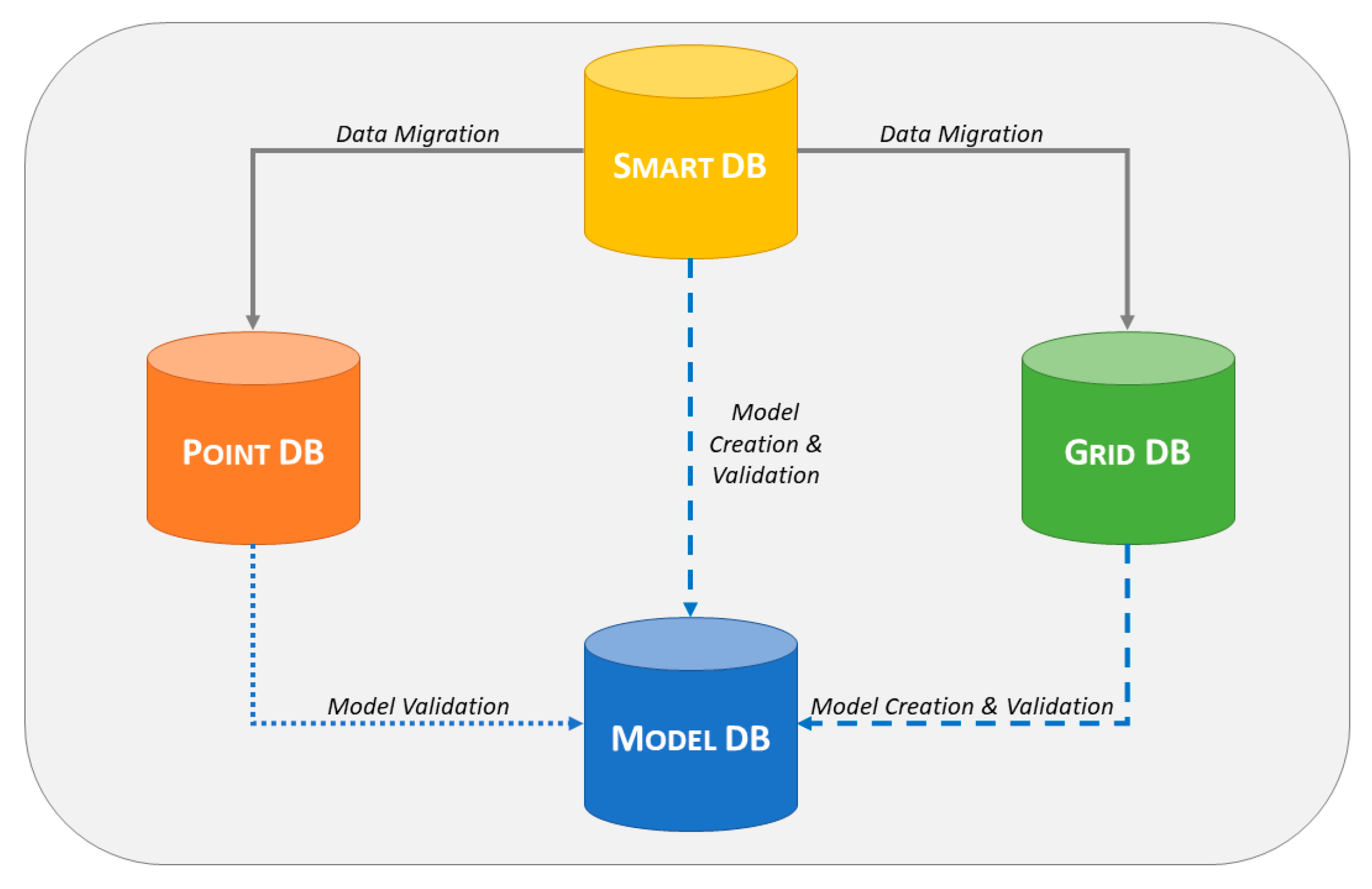
2.1. Management of Data Sources
- Smart DB: The Survey Metadata and Raw data Tracker (Smart) database is used to manage an extensive collection of survey metadata, as well as for storing information used to track the integrity of the acquired raw data.
- Point DB: The Point database primarily contains the point cloud of cleaned soundings collected during the survey. When available in the data input, the soundings removed during the cleaning process are also stored, thus, replicating the original bathymetric content of the acquired raw data.
- Grid DB: Specially designed for dense datasets such as the ones collected by modern MBES, the Grid database contains a subset of the cleaned soundings stored in the Point database, at a spatial resolution tailored for nautical chart production.
- Model DB: Intermediate products and final DBMs are stored in the Model database.
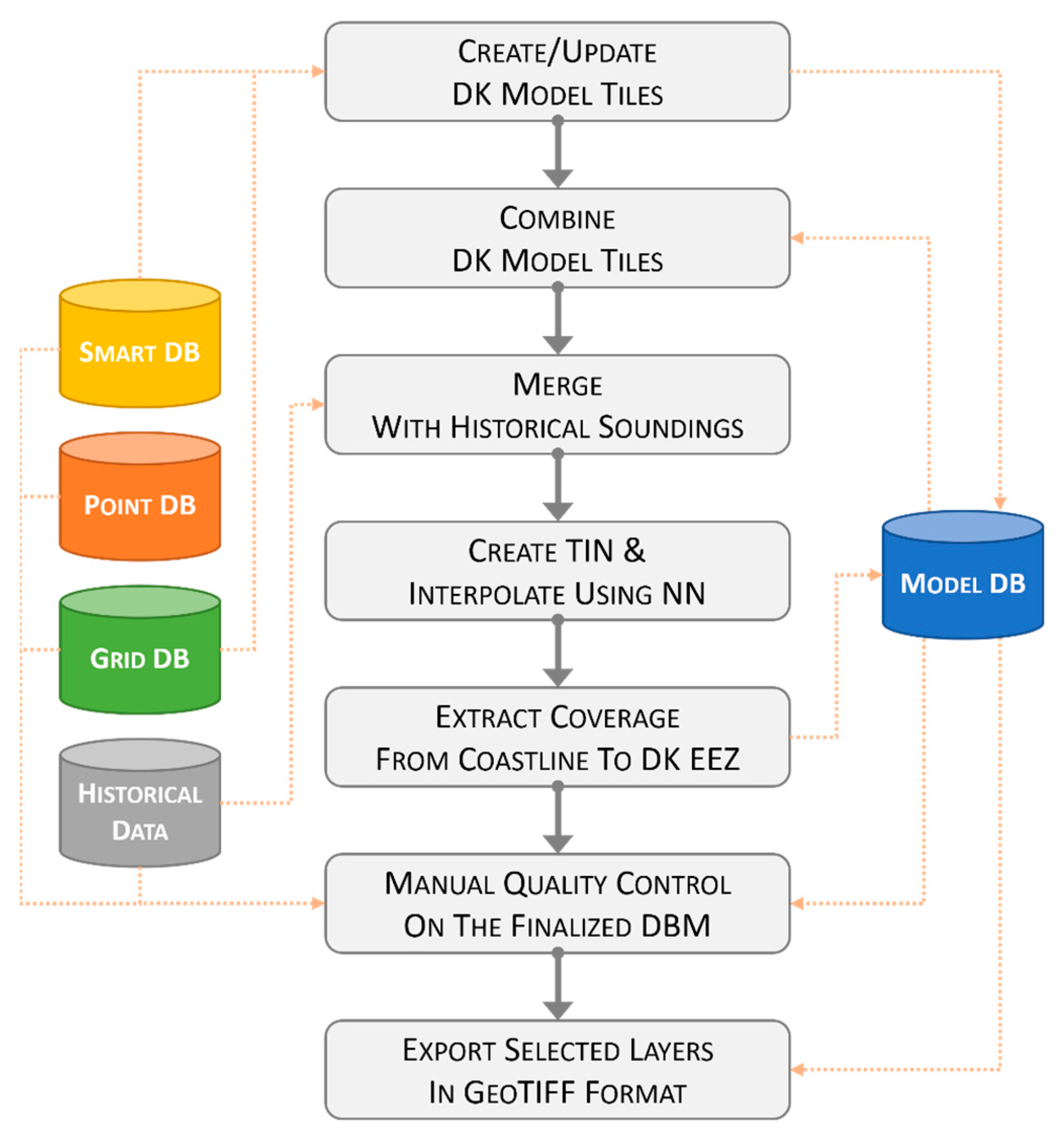
2.2. Compilation Approach
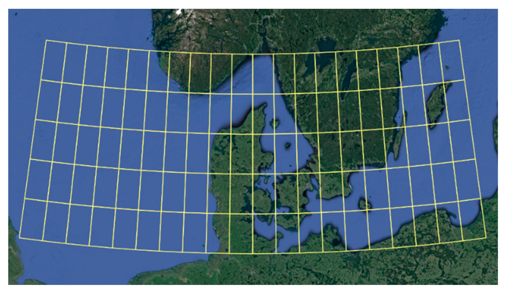
- Creation/update of the model tiles for datasets in Danish waters. The source datasets are retrieved from the Grid DB and related metadata from the Smart DB using the Survey ID. The sources are gridded by adopting a grid resolution of 50 m and a tiling scheme with a tile area of 1° of latitude by 1° of longitude (Figure 3). The tiles covered by at least one dataset are generated and stored in the Model DB. The bathymetric values are calculated as representative average depth, that is, an average of all water depths allocated from the relevant input source to a given grid cell. When multiple datasets overlap, the relevant input source is selected primarily based on the time of data collection. This step is periodically executed to update the tiles in the case of new datasets.
- Combination of the model tiles into a continuous DBM. All the populated DDM tiles stored in Model DB are combined into a continuous DYBDB-sources-only DBM.
- Extension of the continuous DBM with historical soundings. The DBM calculated in the previous step is extended by combining it with historical soundings available on published nautical products.
- Interpolation using a Triangulated Irregular Network (TIN) and natural neighbors. To fill areas with sparse soundings, an interpolated DBM is generated by first creating a Triangulated Irregular Network (TIN) from the extended DBM (generated in the previous step), then using the TIN to interpolate based on the ‘natural neighbors’ algorithm [40,41].
- Coverage extraction based on Denmark’s EEZ. The interpolated DBM is updated to limit its coverage from the coastline (generalized at 1:100,000 scale) to the EEZ. The resulting DBM is uploaded to the Model DB.
- Quality control. The quality of the DBM resulting from the previous steps is extensively assessed by a team of reviewers. During this iterative process, the reviewers have access to all the direct and indirect DBM sources through Smart DB, Point DB, Grid DB, and historical data. In case of issues, adjustments to the model may require the (partial or total) re-execution of the previous steps. Only when the outcomes of the quality control are satisfactory is the DBM finalized.
2.3. Model Products
3. Results
4. Discussion
5. Conclusions
Author Contributions
Funding
Institutional Review Board Statement
Informed Consent Statement
Data Availability Statement
Acknowledgments
Conflicts of Interest
References
- Weatherall, P.; Marks, K.M.; Jakobsson, M.; Schmitt, T.; Tani, S.; Arndt, J.E.; Rovere, M.; Chayes, D.; Ferrini, V.; Wigley, R. A new digital bathymetric model of the world’s oceans. Earth Space Sci. 2015, 2, 331–345. [Google Scholar] [CrossRef]
- Jakobsson, M.; Stranne, C.; O’Regan, M.; Greenwood, S.L.; Gustafsson, B.; Humborg, C.; Weidner, E. Bathymetric properties of the Baltic Sea. Ocean Sci. 2019, 15, 905–924. [Google Scholar] [CrossRef]
- Mayer, L.; Jakobsson, M.; Allen, G.; Dorschel, B.; Falconer, R.; Ferrini, V.; Lamarche, G.; Snaith, H.; Weatherall, P. The Nippon Foundation—GEBCO Seabed 2030 Project: The quest to see the world’s oceans completely mapped by 2030. Geosciences 2018, 8, 63. [Google Scholar] [CrossRef]
- Ryan, W.B.F.; Carbotte, S.M.; Coplan, J.O.; O’Hara, S.; Melkonian, A.; Arko, R.; Weissel, R.A.; Ferrini, V.; Goodwillie, A.; Nitsche, F.; et al. Global Multi-resolution topography synthesis. Geochem. Geophys. Geosystems 2009, 10, 2008GC002332. [Google Scholar] [CrossRef]
- Jakobsson, M.; Mayer, L.A.; Bringensparr, C.; Castro, C.F.; Mohammad, R.; Johnson, P.; Ketter, T.; Accettella, D.; Amblas, D.; An, L.; et al. The international bathymetric chart of the Arctic Ocean version 4.0. Sci. Data 2020, 7, 176. [Google Scholar] [CrossRef]
- Schaap, D.M.A.; Schmitt, T. EMODnet Bathymetry—Further developing a high resolution digital bathymetry for European seas. In Proceedings of the EGU General Assembly 2020, Online, 4–8 May 2020; p. 10296. [Google Scholar] [CrossRef]
- Sandwell, D.T.; Gille, S.T.; Orcutt, J.; Smith, W.H.F. Bathymetry from space is now possible. EOS Trans. Am. Geophys. Union 2003, 84, 37–44. [Google Scholar] [CrossRef]
- Andersen, O.B.; Knudsen, P.; Berry, P.A.M. The DNSC08GRA global marine gravity field from double retracked satellite altimetry. J. Geod. 2010, 84, 191–199. [Google Scholar] [CrossRef]
- Legeais, J.F.; Ablain, M.; Zawadzki, L.; Zuo, H.; Johannessen, J.A.; Scharffenberg, M.G.; Fenoglio-Marc, L.; Fernandes, M.J.; Andersen, O.B.; Rudenko, S.; et al. An improved and homogeneous altimeter sea level record from the ESA Climate Change Initiative. Earth Syst. Sci. Data 2018, 10, 281–301. [Google Scholar] [CrossRef]
- Mayer, L.; Roach, J.A.; Nordquist, M.H.; Long, R. Marine Biodiversity of Areas beyond National Jurisdiction. In The Quest to Completely Map the World’s Oceans in Support of Understanding Marine Biodiversity and the Regulatory Barriers WE Have Created; Brill: Leiden, The Netherlands, 2021; pp. 149–166. [Google Scholar]
- Dierssen, H.M.; Theberge, A.E. Bathymetry: Assessment. In Coastal and Marine Environments; CRC Press: Boca Raton, FL, USA, 2020; pp. 175–184. [Google Scholar]
- de Giosa, F.; Scardino, G.; Vacchi, M.; Piscitelli, A.; Milella, M.; Ciccolella, A.; Mastronuzzi, G. Geomorphological Signature of Late Pleistocene Sea Level Oscillations in Torre Guaceto Marine Protected Area (Adriatic Sea, SE Italy). Water 2019, 11, 2409. [Google Scholar] [CrossRef]
- Westfeld, P.; Maas, H.-G.; Richter, K.; Weiß, R. Analysis and correction of ocean wave pattern induced systematic coordinate errors in airborne LiDAR bathymetry. ISPRS J. Photogramm. Remote Sens. 2017, 128, 314–325. [Google Scholar] [CrossRef]
- Parrish, C.E.; Magruder, L.A.; Neuenschwander, A.L.; Forfinski-Sarkozi, N.; Alonzo, M.; Jasinski, M. Validation of ICESat-2 ATLAS bathymetry and analysis of ATLAS’s bathymetric mapping performance. Remote Sens. 2019, 11, 1634. [Google Scholar] [CrossRef]
- Lurton, X. An Introduction to Underwater Acoustics: Principles and Applications, 2nd ed.; Springer, Published in Association with Praxis Publishing: Chichester, UK; Heidelberg, Germany; New York, NY, USA, 2010. [Google Scholar]
- Hughes Clarke, J.E. Multibeam echosounders. In Submarine Geomorphology; Micallef, A., Krastel, S., Savini, A., Eds.; Springer International Publishing: Cham, Switzerland, 2018; pp. 25–41. [Google Scholar]
- Hughes Clarke, J.E. The impact of acoustic imaging geometry on the fidelity of seabed bathymetric models. Geosciences 2018, 8, 109. [Google Scholar] [CrossRef]
- Masetti, G.; Kelley, J.G.W.; Johnson, P.; Beaudoin, J. A ray-tracing uncertainty estimation tool for ocean mapping. IEEE Access 2018, 6, 2136–2144. [Google Scholar] [CrossRef]
- Lucieer, V.; Lecours, V.; Dolan, M.F.J. Charting the course for future developments in marine geomorphometry: An introduction to the special issue. Geosciences 2018, 8, 477. [Google Scholar] [CrossRef]
- Kjeldsen, K.K.; Weinrebe, R.W.; Bendtsen, J.; Bjørk, A.A.; Kjær, K.H. Multibeam bathymetry and CTD measurements in two fjord systems in southeastern Greenland. Earth Syst. Sci. Data 2017, 9, 589–600. [Google Scholar] [CrossRef]
- Lebrec, U.; Paumard, V.; O’Leary, M.J.; Lang, S.C. Towards a regional high-resolution bathymetry of the North West Shelf of Australia based on Sentinel-2 satellite images, 3D seismic surveys, and historical datasets. Earth Syst. Sci. Data 2021, 13, 5191–5212. [Google Scholar] [CrossRef]
- Thierry, S.; Dick, S.; George, S.; Benoit, L.; Cyrille, P. EMODnet bathymetry a compilation of bathymetric data in the European waters. In Proceedings of the OCEANS 2019, Marseille, France, 17–20 June 2019; pp. 1–7. [Google Scholar] [CrossRef]
- Palmiotto, C.; Loreto, M.F. Regional scale morphological pattern of the Tyrrhenian Sea: New insights from EMODnet bathymetry. Geomorphology 2019, 332, 88–99. [Google Scholar] [CrossRef]
- Sowers, D.C.; Masetti, G.; Mayer, L.A.; Johnson, P.; Gardner, J.V.; Armstrong, A.A. Standardized geomorphic classification of seafloor within the United States Atlantic canyons and continental margin. Front. Mar. Sci. 2020, 7, 9. [Google Scholar] [CrossRef]
- Masetti, G.; Mayer, L.; Ward, L. A Bathymetry- and reflectivity-based approach for seafloor segmentation. Geosciences 2018, 8, 14. [Google Scholar] [CrossRef]
- Koop, L.; Snellen, M.; Simons, D.G. An Object-based image analysis approach using bathymetry and bathymetric derivatives to classify the seafloor. Geosciences 2021, 11, 45. [Google Scholar] [CrossRef]
- Lubczonek, J.; Wlodarczyk-Sielicka, M.; Lacka, M.; Zaniewicz, G. Methodology for developing a combined bathymetric and topographic surface model using interpolation and geodata reduction techniques. Remote Sens. 2021, 13, 4427. [Google Scholar] [CrossRef]
- Włodarczyk-Sielicka, M.; Bodus-Olkowska, I.; Łącka, M. The process of modelling the elevation surface of a coastal area using the fusion of spatial data from different sensors. Oceanologia 2022, 64, 22–34. [Google Scholar] [CrossRef]
- Morlighem, M.; Williams, C.N.; Rignot, E.; An, L.; Arndt, J.E.; Bamber, J.L.; Catania, G.; Chauché, N.; Dowdeswell, J.A.; Dorschel, B.; et al. BedMachine v3: Complete bed topography and ocean bathymetry mapping of Greenland from multibeam echo sounding combined with mass conservation. Geophys. Res. Lett. 2017, 44, 11051–11061. [Google Scholar] [CrossRef] [PubMed]
- Harris, P.T.; Macmillan-Lawler, M.; Rupp, J.; Baker, E.K. Geomorphology of the oceans. Mar. Geol. 2014, 352, 4–24. [Google Scholar] [CrossRef]
- Lecours, V.; Dolan, M.F.J.; Micallef, A.; Lucieer, V.L. A review of marine geomorphometry, the quantitative study of the seafloor. Hydrol. Earth Syst. Sci. 2016, 20, 3207–3244. [Google Scholar] [CrossRef]
- Jakobsson, M.; Mayer, L.A. Polar region bathymetry: Critical knowledge for the prediction of global sea level rise. Front. Mar. Sci. 2022, 8, 788724. [Google Scholar] [CrossRef]
- Hvid Ribergaard, M.; Anker Pedersen, S.; Ådlandsvik, B.; Kliem, N. Modelling the ocean circulation on the West Greenland shelf with special emphasis on northern shrimp recruitment. Cont. Shelf Res. 2004, 24, 1505–1519. [Google Scholar] [CrossRef]
- Moses, C.A.; Vallius, H. Mapping the geology and topography of the European Seas (European Marine Observation and Data Network, EMODnet). Q. J. Eng. Geol. Hydrogeol. 2021, 54, qjegh2020-131. [Google Scholar] [CrossRef]
- Fonseca, L.; Lurton, X.; Fezzani, R.; Augustin, J.-M.; Berger, L. A statistical approach for analyzing and modeling multibeam echosounder backscatter, including the influence of high-amplitude scatterers. J. Acoust. Soc. Am. 2021, 149, 215–228. [Google Scholar] [CrossRef]
- Lebrec, U.; Riera, R.; Paumard, V.; O’Leary, M.J.; Lang, S.C. Automatic mapping and characterisation of linear depositional bedforms: Theory and application using bathymetry from the North West Shelf of Australia. Remote Sens. 2022, 14, 280. [Google Scholar] [CrossRef]
- Vrdoljak, L. Comparison and analysis of publicly available bathymetry models in the East Adriatic Sea. NAŠE MORE Znan. Časopis Za More I Pomor. 2021, 68, 110–119. [Google Scholar] [CrossRef]
- Danish Geodata Agency. National Report of Denmark; IHO Baltic Sea Hydrographic Commission: Monte Carlo, Monaco, 2021. [Google Scholar]
- EMODnet Bathymetry Consortium. EMODnet Digital Bathymetry (DTM); EMODnet Bathymetry Consortium: Brussels, Belgium, 2020. [Google Scholar] [CrossRef]
- Watson, D. The natural neighbor series manuals and source codes. Comput. Geosci. 1999, 25, 463–466. [Google Scholar] [CrossRef]
- Lee, J.A.Y. Comparison of existing methods for building triangular irregular network, models of terrain from grid digital elevation models. Int. J. Geogr. Inf. Syst. 1991, 5, 267–285. [Google Scholar] [CrossRef]
- Ritter, N.; Ruth, M. The GeoTiff data interchange standard for raster geographic images. Int. J. Remote Sens. 1997, 18, 1637–1647. [Google Scholar] [CrossRef]
- Smith, S.M. The Navigation Surface: A Multipurpose Bathymetric Database. Master’s Thesis, University of New Hampshire, Durham, NH, USA, 2003. [Google Scholar]
- Masetti, G.; Rondeau, M.; Baron, B.J.; Wills, P.; Petersen, Y.M.; Salmia, J. Trusted Crowd-Sourced Bathymetry: From the Trusted Crowd to the Chart; Danish Geodata Agency & Canadian Hydrographic Service: Nørresundby, Denmark, 2020. [Google Scholar]
- Desmet, P.J.J. Effects of interpolation errors on the analysis of DEMs. Earth Surf. Process. Landf. 1997, 22, 563–580. [Google Scholar] [CrossRef]
- Florinsky, I. Digital Terrain Analysis in Soil Science and Geology; Academic Press: Washington, DC, USA, 2016. [Google Scholar]
- Masetti, G.; Faulkes, T.; Wilson, M.; Wallace, J. Effective automated procedures for hydrographic data review. Geomatics 2022, 2, 338–354. [Google Scholar] [CrossRef]
- Lecours, V.; Devillers, R.; Schneider, D.C.; Lucieer, V.L.; Brown, C.J.; Edinger, E.N. Spatial scale and geographic context in benthic habitat mapping: Review and future directions. Mar. Ecol. Prog. Ser. 2015, 535, 259–284. [Google Scholar] [CrossRef]
- Lecours, V.; Devillers, R.; Edinger, E.N.; Brown, C.J.; Lucieer, V.L. Influence of artefacts in marine digital terrain models on habitat maps and species distribution models: A multiscale assessment. Remote Sens. Ecol. Conserv. 2017, 3, 232–246. [Google Scholar] [CrossRef]
- Wölfl, A.-C.; Snaith, H.; Amirebrahimi, S.; Devey, C.W.; Dorschel, B.; Ferrini, V.; Huvenne, V.A.I.; Jakobsson, M.; Jencks, J.; Johnston, G.; et al. Seafloor mapping—The challenge of a truly global ocean bathymetry. Front. Mar. Sci. 2019, 6, 283. [Google Scholar] [CrossRef]


| Layer (in Danish) | Description |
|---|---|
| ddm_50m.dybde | The primary layer containing the depth values (in meters). |
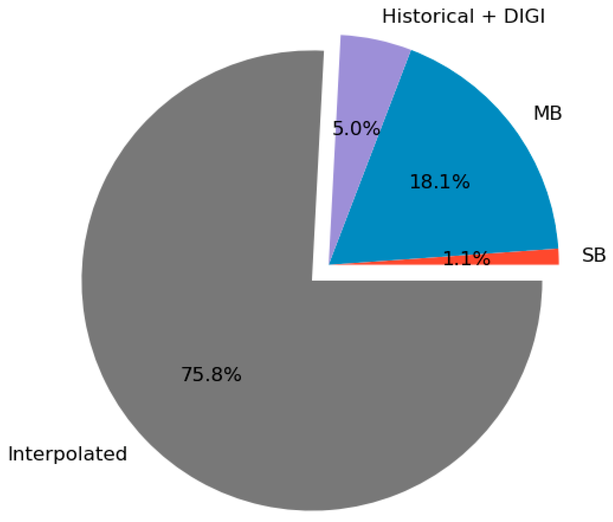
| ddm_50m.kilde | An auxiliary layer providing the source of the depth data for each grid cell. The layer uses the following convention:
|
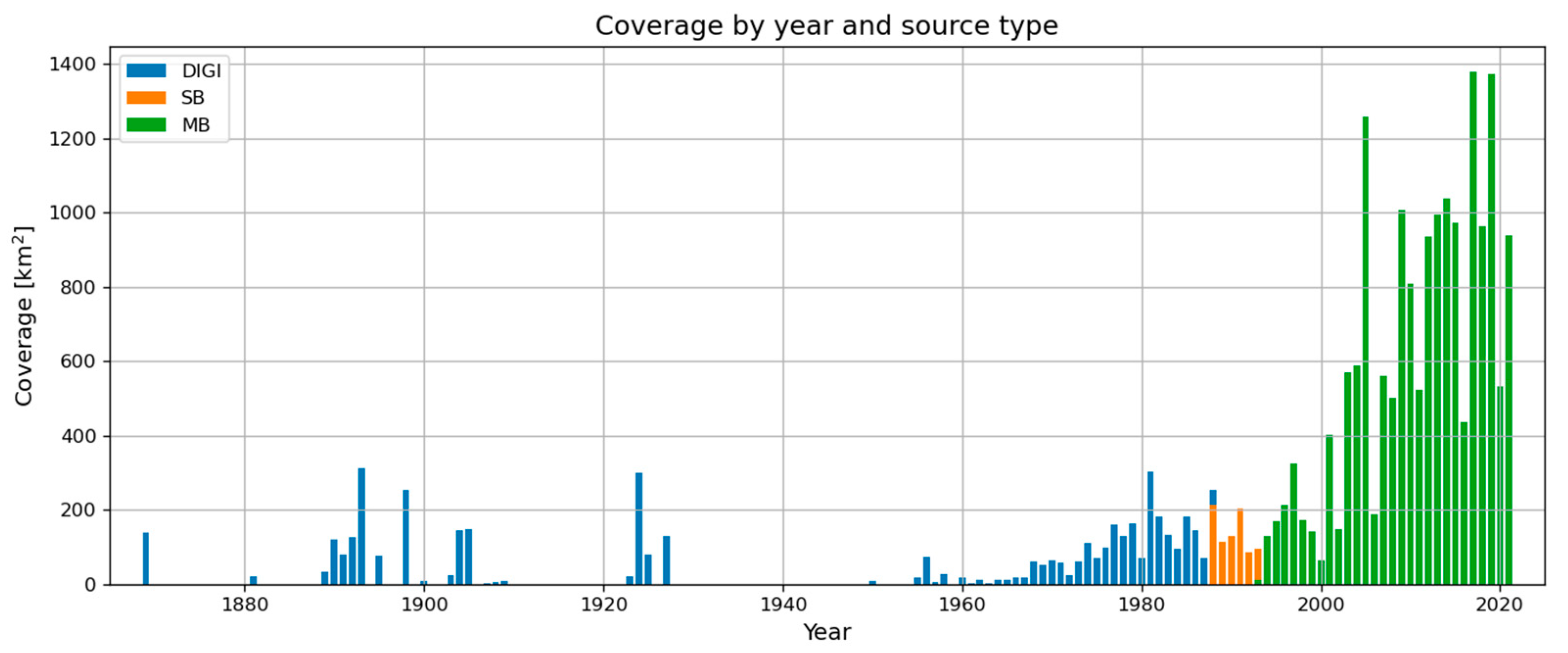
| ddm_50m.aar | An auxiliary layer providing the year at which the data collection has ended (only for DIGI, SB and MB dataset types). |
Publisher’s Note: MDPI stays neutral with regard to jurisdictional claims in published maps and institutional affiliations. |
© 2022 by the authors. Licensee MDPI, Basel, Switzerland. This article is an open access article distributed under the terms and conditions of the Creative Commons Attribution (CC BY) license (https://creativecommons.org/licenses/by/4.0/).
Share and Cite
Masetti, G.; Andersen, O.; Andreasen, N.R.; Christiansen, P.S.; Cole, M.A.; Harris, J.P.; Langdahl, K.; Schwenger, L.M.; Sonne, I.B. Denmark’s Depth Model: Compilation of Bathymetric Data within the Danish Waters. Geomatics 2022, 2, 486-498. https://doi.org/10.3390/geomatics2040026
Masetti G, Andersen O, Andreasen NR, Christiansen PS, Cole MA, Harris JP, Langdahl K, Schwenger LM, Sonne IB. Denmark’s Depth Model: Compilation of Bathymetric Data within the Danish Waters. Geomatics. 2022; 2(4):486-498. https://doi.org/10.3390/geomatics2040026
Chicago/Turabian StyleMasetti, Giuseppe, Ove Andersen, Nicki R. Andreasen, Philip S. Christiansen, Marcus A. Cole, James P. Harris, Kasper Langdahl, Lasse M. Schwenger, and Ian B. Sonne. 2022. "Denmark’s Depth Model: Compilation of Bathymetric Data within the Danish Waters" Geomatics 2, no. 4: 486-498. https://doi.org/10.3390/geomatics2040026
APA StyleMasetti, G., Andersen, O., Andreasen, N. R., Christiansen, P. S., Cole, M. A., Harris, J. P., Langdahl, K., Schwenger, L. M., & Sonne, I. B. (2022). Denmark’s Depth Model: Compilation of Bathymetric Data within the Danish Waters. Geomatics, 2(4), 486-498. https://doi.org/10.3390/geomatics2040026