Article

Comprehensive Analysis of Ocean Current and Sea Surface Temperature Trend under Global Warming Hiatus of Kuroshio Extent Delineated Using a Combination of Spatial Domain Filters

by
Mohammed Abdul Athick AS
1,2,3 and
Shih-Yu Lee
3,*
1
Taiwan International Graduate Program (TIGP), Earth System Science Program (ESS), Academia Sinica, Taipei 11529, Taiwan
2
College of Earth Sciences, National Central University, Taoyuan 32001, Taiwan
3
Research Center for Environmental Changes, Academia Sinica, Taipei 11529, Taiwan
*
Author to whom correspondence should be addressed.
Geomatics 2022, 2(4), 415-434; https://doi.org/10.3390/geomatics2040023
Submission received: 10 August 2022 / Revised: 21 September 2022 / Accepted: 22 September 2022 / Published: 25 September 2022

Abstract

:
The effect of climate prevails on a diverse time scale from days to seasons and decades. Between 1993 and 2013, global warming appeared to have paused even though there was an increase in atmospheric greenhouse gases. The variations in oceanographic variables, like current speed and sea surface temperature (SST), under the influence of the global warming hiatus (1993–2013), have drawn the attention of the global research community. However, the magnitude of ocean current and SST characteristics oscillates and varies with their geographic locations. Consequently, investigating the spatio-temporal changing aspects of oceanographic parameters in the backdrop of climate change is essential, specifically in coastal regions along Kuroshio current (KC), where fisheries are predominant. This study analyzes the trend of ocean current and SST induced mainly during the global warming hiatus, before and till the recent time based on the daily ocean current data from 1993 to 2020 and SST between 1982 and 2020. The Kuroshio extent is delineated from its surrounding water masses using an aggregation of raster classification, stretching, equalization, and spatial filters such as edge detection, convolution, and Laplacian. Finally, on the extracted Kuroshio extent, analyses such as time series decomposition (additive) and statistical trend computation methods (Yue and Wang trend test and Theil–Sen’s slope estimator) were applied to dissect and investigate the situations. An interesting downward trend is observed in the KC between the East coast of Taiwan and Tokara Strait (Tau = −0.05, S = −2430, Sen’s slope = −5.19 × 10⁻⁵, and Z = −2.61), whereas an upward trend from Tokara Strait to Nagoya (Tau = 0.89, S = 4344, Sen’s slope = 8.4 × 10⁻⁵, and Z = 2.56). In contrast, a consistent increasing SST in trend is visualized in the southern and mid-KC sections but with varying magnitude.

Graphical Abstract

1. Introduction

The ocean and atmosphere are crucial elements of the Earth system. Therefore, the thermo-physical properties of the oceans and their current speed are essential components in oceanographic and climate studies. Sea surface temperature (SST), land surface temperature, precipitation, wind pattern, ocean current, relative humidity, and their interactions lead to the statistical mean variability of average weather from days to months or seasons and thousands of decades [1,2]. As the solar radiation constantly heats the ocean surface between 23.5° N and 23.5° S. Kuroshio, a western boundary current, is vitally essential to transport and modulate the surplus thermal content of the ocean from the tropics to poleward (north).
The heat and transport by Kuroshio extension (Kuroshio between 30° to 40° N and 140° to 180° E) appeared to have been enhanced by global warming during the past 100 years. Moreover, the analysis of multiyear SST and volume transport by the Kuroshio current (KC) was a vital challenge. However, diverse resources, for instance, cruise vessels, models, satellite, and Argo providing high resolution multiple datasets for in-depth data examination, revealed a shift in the path of Kuroshio extension [3]. Because of SST’s connection to global warming, the rising sea temperature has received a lot of attention [4,5]. Since 1971, there has been a linear trend of 10.1 °C/decade in the global mean temperature at a depth of 75 m [5,6]. Given that the surface ocean reacts immediately to atmospheric warming, SST is one of the crucial elements in determining how warming occurs. Long-term remote sensing data on SST are also accessible. However, SST warming is not regionally uniform, which is significant. Previous research has found that the western boundary currents are particularly quickly warming [3,7]. Understanding the causes behind this rapid warming is crucial to comprehending climate change [8,9]. The atmosphere is significantly impacted by SST fluctuation in the East China Sea [10,11,12,13]. The SST pattern of the East China Sea is the subject of several research [3,14,15,16].
The East Asian monsoons influence KC’s kinetic energy (magnitude of current) on a seasonal scale. On the other hand, the impact of extreme weather events (El Nino and La Nina) lasts on an inter-annual scale [17]. These seasonal and inter-annual climatic variations direct to regional scale modifications of surface winds at 10 m over the North Pacific. This further influences KC water masses’ southward and northward transportation in the deep ocean and western boundary, respectively [17]. Likewise, a decadal scale rise in eastward transport of the KC in the south of Japan was also documented [18]. Miller et al. [19] diagnosed and verified these decadal scale deviations of KC. Most of the research on Kuroshio intensity used hydrography data collected from cruise ships, KC transport, ocean circulation models, or sea surface height differences to quantify the strength of KC [3,17,18,19]. An increasing KC trend would benefit us more in a perfect scenario by moving more heat poleward. At the same time, the decreasing trend in KC would impact the regional scale weather of Taiwan, the Philippines, and Japan. In addition, global analysis to understand past and co-occurring climate change has attracted significant attention [20]. Despite the fact that the levels of greenhouse gases in the atmosphere have risen, the global warming rate has slowed down or paused, or hiatus since the late 1990s [21,22].
The downshift in global warming resembles the renowned Pacific Decadal oscillation’s negative phase in many ways [23]. However, it may not be a perfect match because the former may also be influenced by feeble solar activity [24], reduced stratospheric moisture [25], enhanced volcanic outbursts [26], surged stratospheric aerosols [27], increased ocean thermal storage capacity [28], and cooling of the central-eastern tropical Pacific [22,29,30]. The negative Pacific Decadal oscillation and the simultaneous strengthening of prevailing winds (trades) in or around the end of the 1990s are primarily cited as significant dual contributors to these advancements, despite their diversity. In actuality, the Kuroshio strength was more influenced by the wind stress curl, and Pacific Decadal oscillation, than by the net thermal intake made things more difficult. The Kuroshio modifies the climate by transferring extra heat from the tropics to the poles. Additionally, it impacts typhoons’ growth, the fishing industry’s profitability, and ocean circulation in nearby marginal areas like the East and the South China Sea. As a result, the Kuroshio had higher incursion occurrences when it weakened and had a more significant influence [31,32,33,34,35,36].
The Kuroshio front was generally identified by researchers in the conventional rectangular or square domain. The two-dimensional histogram, in conjunction with the SST and chlorophyll-a ranges, was used by Takahashi and Kawamura to analyze the seasonal fluctuation of Kuroshio [37,38]. However, the objective technique [39] is capable of spatially detecting ocean fronts. The abrupt gradient regions, also known as edges, originated due to the diverse physical processes such as open ocean mixing, upwelling, and convergence are detected during spatial mapping using an objective spatial filter approach. However, due to homogeneous surface heating, the traditional technique employing isotherms outlined above did not function effectively during the summer.
Similarly, extracting features by just specifying an array of values refrains from defining the precise border of Kuroshio [38]. Boundary identification, cluster shadow method, and entropic approach are the most efficient and functional techniques for separating a feature from its surroundings. In addition to objective gradient filters, image classification algorithms, especially the standard deviation and Jenks procedure, are repeatedly employed in remote sensing. These image processing approaches to spatially identify a feature precisely in remote sensing satellite data are incomprehensible to recognize. In a similar vein, the histogram equalization and gradient detection filter are two extensively used techniques because of their robustness, sufficient global validation, simplicity, and ease of use [38].
Evaluating SST and ocean current trends across time and space is crucial for planning marine resources and regional decisions [40,41]. In considerable studies, numerous investigations followed through to find the geographical and time-dependent variations [42,43,44].
Many statistical techniques, such as the Mann–Kendall (MK) test, Hamed and Rao modified MK test, and Yue and Wang Modified MK Test, have been devised and used by several studies to analyze the trend [45]. A swift research of these methods has shown that parametric and non-parametric approaches frequently remain available to identify meaningful patterns from multiyear data [46,47]. Only a few time-series change detection/trend analysis techniques have been developed for remote sensing data despite the fact that the importance of satellite multiyear and seasonal images to identify the changes in land-use classes has been well-recognized [48].
Two significant obstacles while examining satellite data are discovering variations within the entire multiyear time-series data and simultaneously considering seasonal shifts into account; therefore, suitable methodologies must first be developed. Since time series contains seasonal, steady, and sudden shifts, in addition to residuals originating through relic geometric/dimensional errors, air dispersion, and cloud coverage/effects, quantifying the change from remotely sensed data are not straightforward [49]. The long-term series decomposition analysis techniques separate the signal from the noise based on temporal features. Still, they also entail some adjustments intended to focus on the primary sources of fluctuation in the multi-temporal spectral space over years of imaging [50]. The MK test is considerably employed without relying on preconceptions for spotting strong unmodulated patterns in time series. The hypothesis for this test signifies an increasing or a decreasing tendency based on a one/two-sided test, but the null hypothesis indicates no trend [51].
In contrast, a study investigating the practicality of MK’s approach to identifying the declination of software performance. Using the computer metrics indicated the MK as an insignificant test; on the other hand, the experimental findings pointed out that using the MK trend analysis to notice the aging of software is favorably revealed, initiating false positives [52]. Nevertheless, other research has utilized the MK’s approach to evaluate temporal and regional trends, such as those conducted in Iran, Kansas, the United States, and is employed in non-parametric tests globally to identify unmodulated patterns in a series of climate data [53,54]. These non-parametric techniques have many advantages in processing time series with missing data, but with few hypotheses and the freedom of data dispersal [55,56,57].
However, the main drawback is the influence of auto-correlation on the test significance of the data. Several researchers have proposed modifying these tests to eliminate auto-correlation using diverse methodologies. One of the most popular assessments is to adjust bias before pre-whitening [58,59,60]. Thus, the MK test is mainly preferred to examine the time series of climatic data considering that its statistical analysis refrains from following the normal distribution.
Ideally, the MK statistical test is a standard method for determining the significance of a trend in time series datasets. However, sample data must be serially independent in order to pass the test. The capacity of the MK test to accurately determine the significance of the trend will be affected by the existence of serial correlation in time series and when sample data are serially correlated. Serial correlation often has an impact while analyzing trends on time series data. Therefore, modified MK tests should be used for trend detection in circumstances when the time series is not random and has been influenced by auto-correlation. Yue and Wang suggested a procedure to correct variance during trend analysis of serially correlated data. First, adequate specimen length is specified using the coefficients of significant serial correlation after eliminating the trend from multiyear time series [61].
Another non-parametric technique frequently employed to specify the amplitude of a trend is the Theil–Sen slope estimator approach. However, characterizing a notable trend in a time series is crucial in trend identification and investigations. Consequently, Sen’s slope estimates the intercept and the gradient [62]. These tests are favored over other tests due to their effectiveness in processing multiyear data, disobeying the statistical dispersion. They are well-reported in the numerous results of time-series studies as an applicable trend test for efficacious investigation of periodic and year-long trends in climate data. Several applications for the time series patterns have been identified using the MK trend analysis, demonstrating inter/intra-annual variability [63]. However, few studies examined extreme temperature, precipitation trends, and their statistical significance using both MK and Sen’s slope estimator over the land as well as the Mediterranean and Black Sea [64,65,66,67,68,69,70,71].
The primary objective of this study is to analyze the trend of SST and ocean currents of Kuroshio extent under global warming hiatus. Based on the data availability, the investigation was extended till 2020. As the SST data are available from 1982, we investigated the trend before, during hiatus, and until recently. On the other hand, the ocean current provided by the Copernicus-GlobCurrent database is from 1993, so the trend analysis was done from 1993 to 2020. Foremost, we employ SST and Ocean current multi-sensor satellite-driven datasets and image processing spatial filters to demarcate the Kuroshio from its surrounding water masses. Then, regarding the Kuroshio extent, the time series decomposition was employed, followed by investigating the trend of SST and Ocean current incorporates comprehension of temperature and magnitude tendencies. Next, the variability was examined using the Yue and Wang Modified MK Test to investigate the unmodulated patterns and, finally, the Sen’s slope estimator to quantify their magnitude. Apprehending the unpredictability corresponding with SST and current patterns will provide an understanding of Kuroshio’s strength and associated wind patterns.

2. Data and Methods

2.1. Study Area

The Kuroshio regulates climate by carrying surplus heat from the tropic to the pole. By advecting a significant quantity of heat from the tropics to the northern mid-latitudes, KC plays a crucial role in the north Pacific circulation, moving seawater with a volume equal to 6000 big rivers. The study area is between 18° to 35° N and 115° to 138° E, where KC streams alongside the eastern Taiwan nearshore towards the continental shelf. Then, Kuroshio transits the Tokara Strait, advancing along Nagoya contouring at a depth of 200 m to 2000 m, transporting 16–26 °C skin SST range by 0.22 and 1.05 m/s ocean current time series data. Therefore, any change in KC’s trajectory or its velocity can have an impact on large- or small-scale climatic changes (Figure 1).

2.2. Data

The input comes from the daily data collected by several satellite missions. Again, however, only data spanning the research region have been used; all datasets given have a global geographic resolution.

2.2.1. Ocean Currents

Copernicus-GlobCurrent Level-4 three hourly, daily, and monthly mean geostrophic and the Ekman current products are used to generate the regional and global surface currents products, which are delivered on 0.25° × 0.25° and produced over the 1993 to 2020 (https://resources.marine.copernicus.eu/, accessed on 2 May 2022).
The geostrophic, Ekman, tidal, and Stokes drift currents are shown in the global perspective at 0 and 15 m of depth. The sum of the geostrophic and Ekman currents equals the total current at 15 m of depth given by:
U c o m b i n e d ( z = 15   m ) = E a s t w a r d g e o s t r o p h i c + E a s t w a r d E k m a n ( z = 15   m ) V c o m b i n e d ( z = 15   m ) = N o r t h w a r d g e o s t s r t o p i c + N o r t h w a r d E k m a n ( z = 15   m )
The resultant ( U 2 + V 2 ) of zonal ( U = E a s t w a r d c o m b i n e d ) and meridional ( V = N o r t h w a r d c o m b i n e d ) current components of ocean currents products at 15 m depth are employed in the present analysis, even though the mere addition of geostrophic and Ekman current does not yield the surface current [72,73,74].

2.2.2. SST

This research employed high-resolution skin SST of the sea surface water from 1982 to 2020 daily averaged version 2.1 of Optimum Interpolation SST (OISST) data with a spatial resolution of 0.25° latitude by 0.25° longitude grids (https://www.ncei.noaa.gov/, accessed on 2 May 2022). It combines in-situ (buoy, Argo float, and ship) with Advanced Very High-Resolution Radiometer (AVHRR) SST. In order to obtain worldwide coverage, the optimum interpolation method fills gaps in geographical data [75,76,77,78].

2.2.3. Ocean Vector Winds
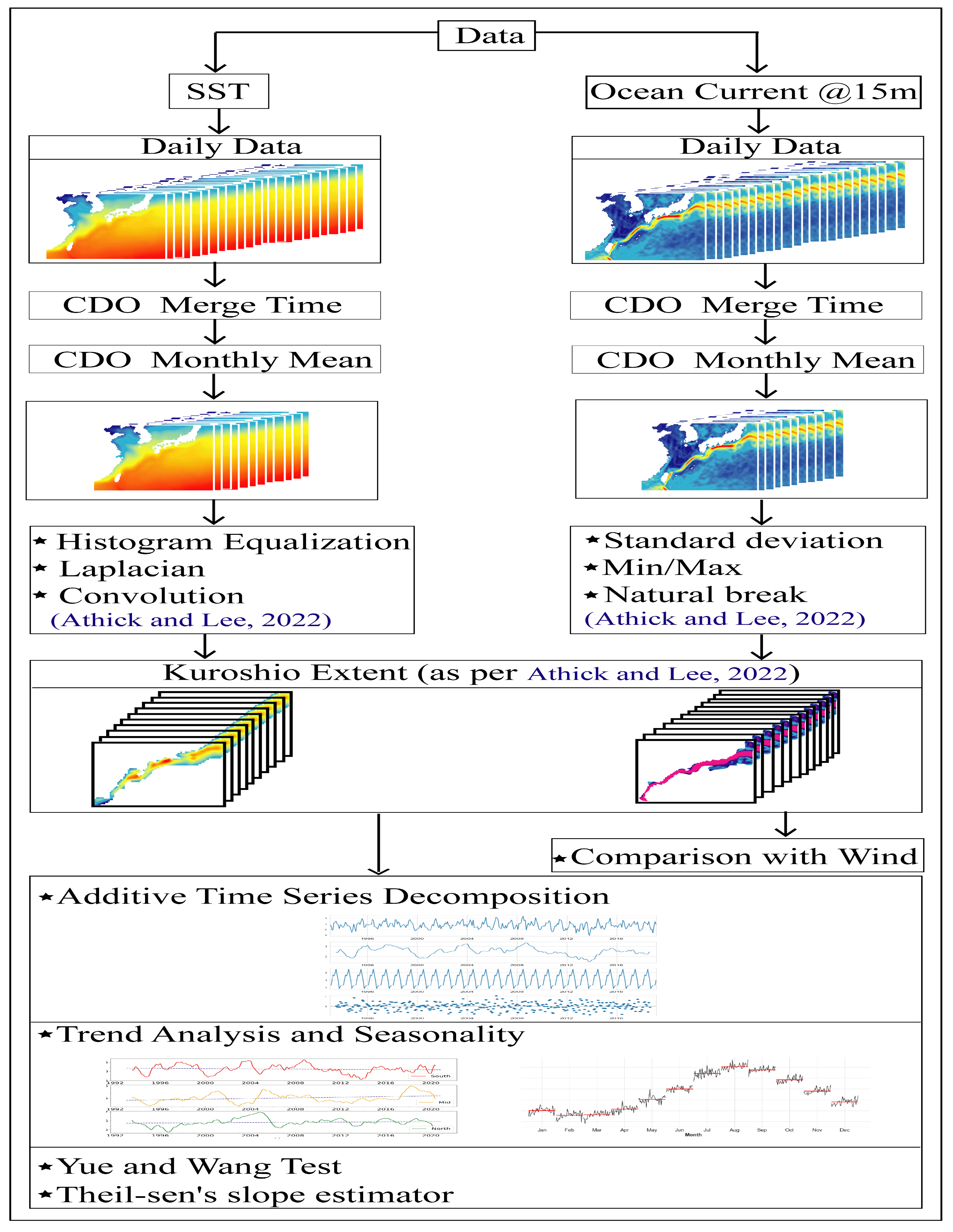
Data from QuikSCAT, ASCAT scatterometer, moored buoy, radiometer, model Variational Analysis Method (VAM), and ERA-Interim winds are merged as Level-3 cross-calibrated multi-platform (CCMP) ocean vector wind of daily resolution with 0.25 degree gridded vector winds between 1993 to 2020 are used in this study (https://www.remss.com/, accessed on 2 May 2022).
Investigating the physical phenomenon between large-scale air and sea moreover their influence on the atmosphere and the ocean requires high-quality ocean surface wind data without gaps with finer temporal and geographical resolution. In addition, ocean vector wind data must be collected for a sufficient amount of time to resolve wind-induced patterns like the El Nino-Southern Oscillation (ENSO) and the Madden-Julian Oscillation (MJO). Ocean winds are dynamic and frequently vary over concise time intervals. Therefore, it is challenging to produce global, gridded, gap-free wind fields due to this property, specifically at temporal and spatial scales lower than common wind characteristics [79,80,81].

2.3. Methods

Figure 2 represents the across-the-board method using an assorted spatial filter and the raster classification method used in this research to delineate Kuroshio from its surrounding water masses. Moreover, this section explains the convoluted methodology with substantial raster pre-processing [82,83], followed by the trend analysis in this research.
Daily mean is utilized to map the relationship of the aforementioned data sets across KC in the research region and was used to calculate the monthly climatologies. We used a multi-variate proposal to detect Kuroshio. First, the augmentation of spatial signatures at fronts connected to the feature is disclosed by employing contextual filters and data classification techniques for remote sensing images. Next, edge detection is used to delineate the KC from remote sensing images. Then, all the images must have been digitally examined and combined with filters to minimize noise while maintaining the features and finally analyzing the trend, followed by exploring the wind pattern over the Kuroshio; Figure 2 shows the hierarchy of data processing methods.

2.3.1. Delineation of Kuroshio

We initially chose the datasets on the first day they were made available. The remainder is filtered to exclude those that do not begin in January and terminate in December. Thus, all datasets have been completed in 12 months while computing monthly climatology.
A convolution and Laplacian filters are fit to process the SST climatological datasets in assortments to extract the KC. These operations execute filtering on a pixel ground to sharpen the feature and detect the edges within a satellite image. Our filters’ primary ingenious technique is that they evaluate a 3 × 3 pixel kernel at a time within a larger, more thorough pixel window. The edges of the features are preserved and enhanced while erroneous data are removed using the overlapping kernel of the convolution filter with 3 × 3 window [84].
By predicting the weighted pixels in their neighborhood, convolution filters work. In oceanography, the foremost contextual approach of filtering was applied to validate large-scale climatological records gathered from the North Pacific Ocean and categorize vertical profiles [85,86]. Without respect to edge direction, a second derivative of the Laplacian filter is further used to improve the detection of KC.
The climatological pixels (I) on the (x) and (y) axes were filtered through the Laplacian filter (L) [87] given by:
L ( X , Y ) = 2 I X 2 + 2 I Y 2
Using a pixel window with a high center value that is often surrounded by zeros at the corners and negative odd pixel window weights in the north–south and east–west pixel directions:
= 0 1 0 1 4 1 0 1 0
Similar to contrast stretching, histogram equalization uses additional repetitive values to portray more contrast. As a result, it describes the regions with the highest frequency of pixel values. As a consequence, the SST spectral signature of pixels in KC, where values occur less often, is improved more than those in the original histogram.
Depending on the data type, a different categorization technique is employed; min-max stretch and Jenks classification (natural break) are used to process sea surface current data. Additionally, we chose the clusters to ensure the dispersion properties of the raw input images are preserved and can be accurately stated using Osaragi’s approaches [88].
The Natural Breaks categorization separates the breakpoints by looking for groupings and patterns in the data. This is the most well-known technique for reducing variance within the data class in spatial analysis. Finally, in order to radiometrically enhance the satellite images and make Kuroshio visible to the human eye, attributes including brightness, contrast, and gamma are adjusted using the minimum-maximum and histogram equalized stretches’ functions. The initial lower and upper limits of the original data are allocated to 0 and 255 on display in the min-max, which is a linear contrast stretch. In some datasets, the vast majority of pixels lie between upper and lower bounds. Thus, we eliminated the extreme values.

2.3.2. Trend Analysis

The term “trend” refers to the long-term shift in the dependent variable over a significant amount of time or the overall movement of a series over a substantial amount of time [89]. For the importance of the trend of SST and ocean current, statistical techniques like regression analysis and the coefficient of determination are applied. In addition, Jan et al. suggested an additive time series decomposition method to suit models of linear and seasonal trends to apply to climate data [50].
T i m e S e r i e s D a t a t = T r e n d t + S e a s o n a l i t y t + R e m a i n d e r t t = 1 , . . . . . . . . , n
The remaining data deviation outside of seasonality and trend makes up the remainder component [90]. The intercept and slope of successive linear representatives, α j and β j , can emanate the extent and direction of the sudden change and the gradient of the step-by-step transition between perceived breakpoints, where the T r e n d t is:
T r e n d t = α j + β j t
and the magnitude is represented as:
M a g n i t u d e o f a b r u p t c h a n g e = ( α j 1 α j ) + ( β j 1 β j ) t
In addition, β j 1 and β j are the gradients of the progressive shift, respectively [91].

2.3.3. Yue and Wang Modified MK Test

The MK test maintains the fundamental condition that the data must be independent despite being reasonably practical and resilient. In other words, serial correlation, which might be statistically influential in some hydrological and climatic time series data, is not robustly noticed by the MK test.
On the other hand, the data’s positive serial correlation will cause the null hypothesis—that there is no trend to be overly rejected, including long-been debated and well-documented. Involving pretreatment of the data and modifying the MK test to report for serial correlation are the two primary strategies that have been recommended to reduce the effect of serial correlation.
Yue and Wang proposed an effective variance correction method for evaluating the data, such as ocean current and SST, with the nature of serial autocorrelation employed in this research. Hence, this research employs a correction method for evaluating the data with the nature of serial autocorrelation [61].

2.3.4. Theil–Sen’s Slope Estimator

Sen’s slope estimator is a technique for simple linear regression in non-parametric statistics by picking the median of all line gradients across tandems of points. Several publications have used the Sen slope to specify trends’ extent and movement (upward/downward).
The main benefit of the Thiel–Sen slope is that it can be computed quickly and is not affected by deviation. Compared to weak basic least squares, it can be a lot more precise for skewed and heteroskedastic data; moreover, it can rival least squares even for properly dispersed data in terms of statistical power [92,93]. This determines the slope of lines using:
S l o p e = m e d i a n { y i y j x i x j } f o r a l l i j

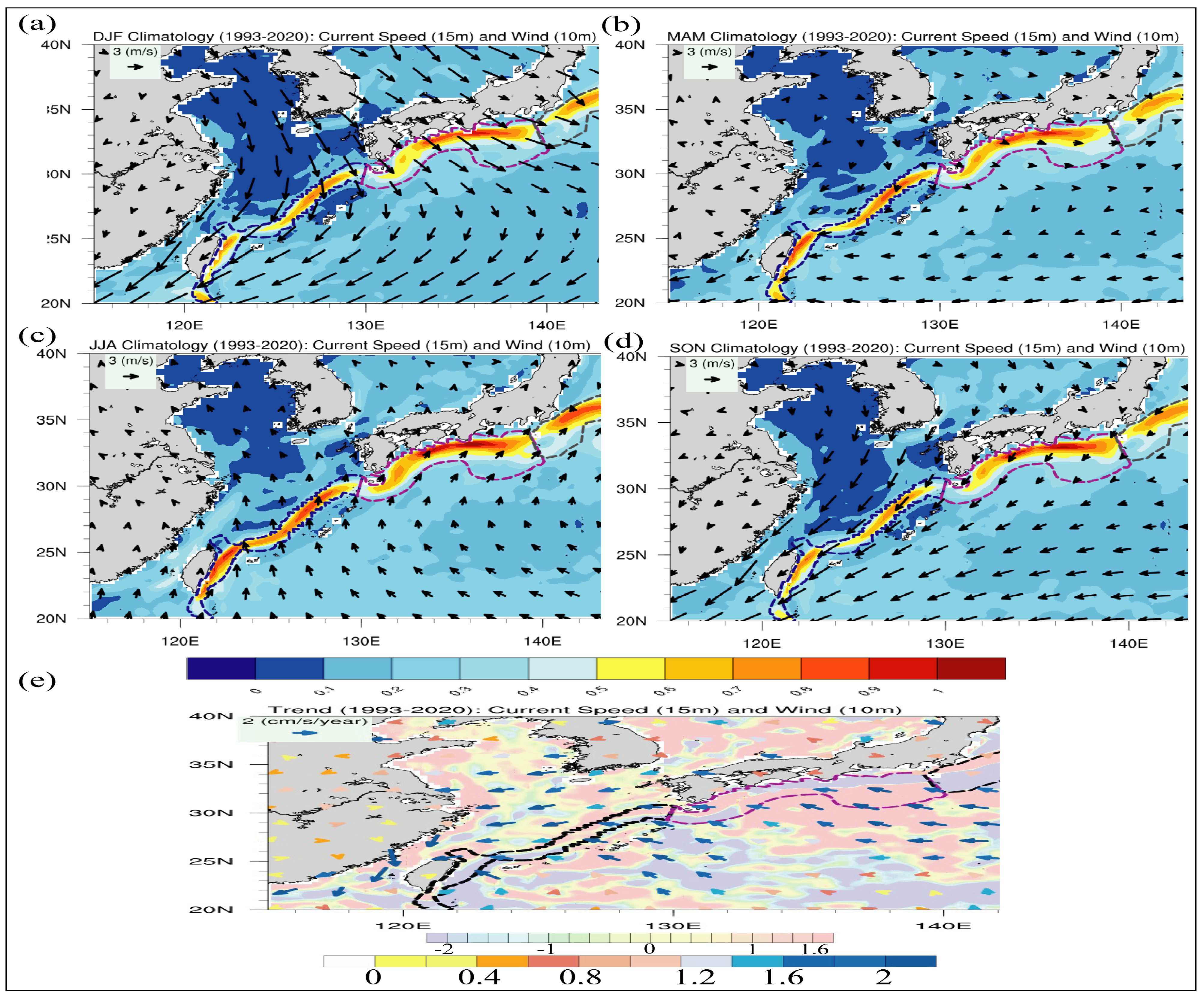
2.3.5. Wind Climatology

Finally, this research used monthly climatological CCMP winds from 1993 to 2020. First, the long-term trend of ocean surface winds presents the synoptic perspective of wind magnitude and velocity over the KC on regional and seasonal peculiarities. Then, the relationship between wind speed and KC’s path and velocity is presented with connections for the investigation of global climate change. The surface-relative wind speeds from the satellite and combined datasets were neutral, comparable, and calibrated to a recommended 10 m level. However, the approximation of wind speed might differ more than was essential for precise aiming, relying on the equilibrium of the atmosphere and the ocean currents [94].

3. Results

3.1. Detection of KC Front

The chosen datasets from the very first day that they were made available were filtered to exclude those that do not begin in January and terminate in December. As a result, all datasets included in the climatology (monthly) computation have a full year of data. Last but not least, we evaluated the algorithms in the range of 18° to 35° N and 120° to 140° E.
Initially, we employed the methodology of using a combination of spatial domain filters [38] to delineate Kuroshio current from its neighboring water masses as the method recommended by Wang [95]. Liu and Hou [96] did not effectively unveil Kuroshio in both x- and y-directions and as well as in summer due to uniform heating. Still, they can be used in detecting the tongue of KC. From each delineated Kuroshio extent for ocean current and SST, the study area is subdivided into two (i.e., from the East coast of Taiwan to Tokara Strait and from Tokara Strait to Nagoya, Japan) (Figure 3).
The KC extent from daily data converted to monthly climatology of ocean current at 15 m between 1993 and 2020 (Figure 3a,b) and skin SST from 1982 to 2020 is illustrated in (Figure 3c,d) using close to 9855 and 13,870 NetCDF images, respectively. The mean climatological skin SST is around 23.6 °C, and the 27 years’ mean climatological current velocity at 15 m depth in the KC extent is between 0.1 to 1.05 ms−1.
The combination of spatial filters, raster algorithms for classification, queries, delineation strategies, and digital image analysis methods can effectively map seasonal and climatology SST and ocean currents of 38 and 27 years, respectively.

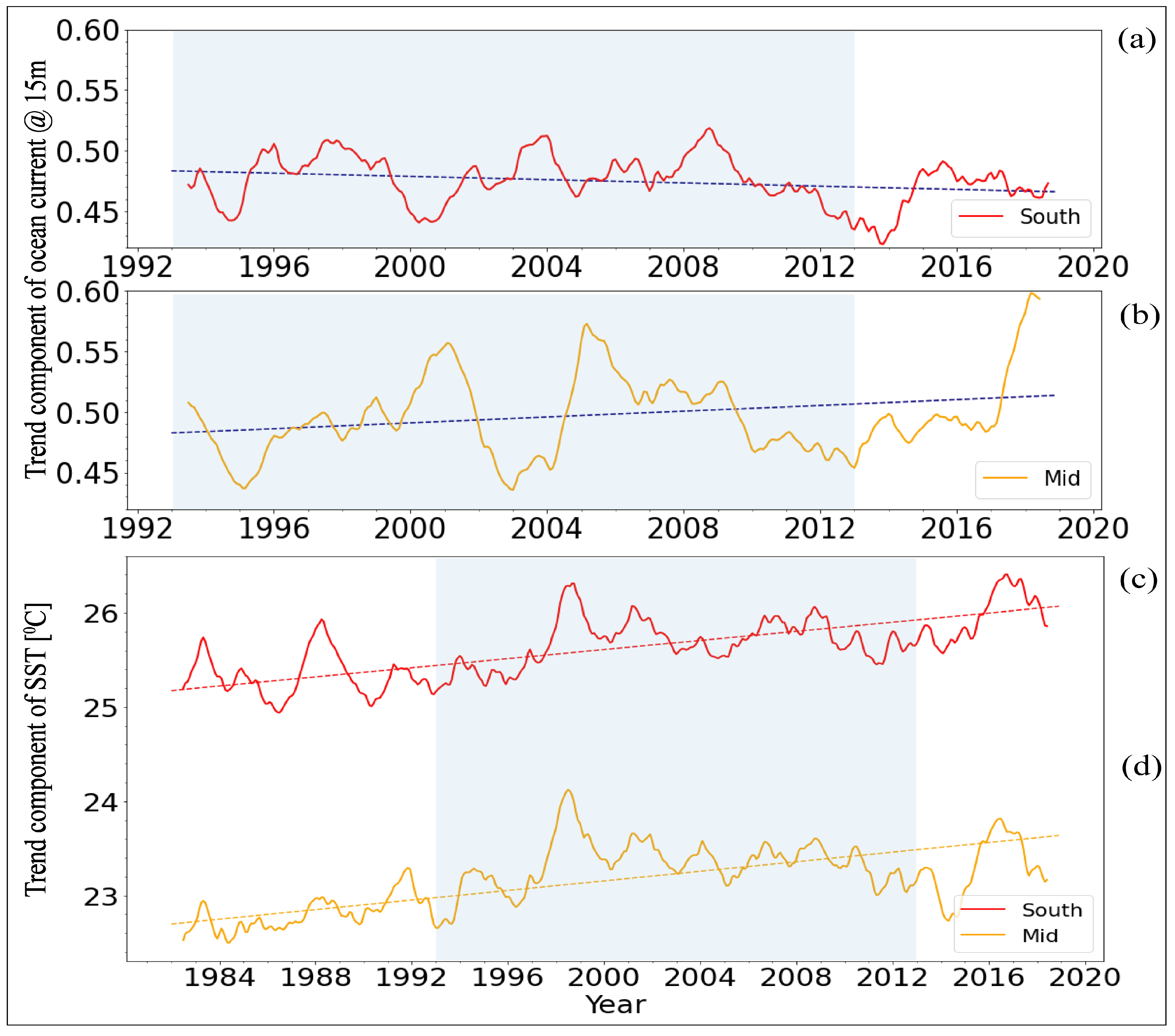
3.2. Time Series Decomposition

We employed an additive time series decomposition model to the NetCDF datasets of SST and ocean current provided in combination with remote sensing, buoy, ships, and as well by algorithms to yield time series to analogize and glimpsed modification with a spatial validation. Table 1 depicts the statistical dispersion of SST and ocean current in the different segments of KC.
The decomposition model yields information on the numeral, temporal stamps, seasonality, extent, and direction of changes in the trend component. Our primary emphasis is on the significant changes occurring within the trend. Last but not least, the residual component can be utilized for prediction and forecasting using machine learning algorithms. The decomposition model fits different time series of SST and ocean current components to precisely estimate the magnitude and trend. The seasonality is decomposed from the raw data using the asymmetric Gaussian function [97].
From Table 1, it can be inferred that, for the auto-correlated datasets, the observed values of mean and 50% of percentile are pretty close. (Figure 4a,b) Moreover, Figure 4c,d illustrate the additive time series decomposition of ocean current and SST between the east coast of Taiwan to Tokara Strait and Tokara Strait to Nagoya, respectively.
The model decomposed the time series data in seasonality, trend, and residual, as the primary focus of this research is to examine the trend. The trend component is statistically analyzed further.

3.3. Trend Computation Using Yue and Wang Modified MK Test and Theil–Sen’s Slope Estimator

The trend component of SST is examined using 38 years of skin SST data from between Taiwan to Tokara Strait and Tokara Strait to Nagoya (1982–2020), along with 27 years of ocean current at 15 m depth of similar spatial extent (1993–2020). In addition, Yue and Wang’s approach and Theil–Sen’s estimator have been employed to confine the SST and current trends. Figure 5a,b illustrates the comparison of the trend component of ocean current between the two sections of KC.
On the other hand, Figure 5c,d show the trend of SST for the same geographic extent. The positive ‘Z’ value of ocean current between Tokara Strait to Nagoya indicates an increasing and upward trend over time. This also suggests a considerable increase in the direction at a 5% significance (Table 2). The ‘Z’ value of the Taiwan to Tokara Strait for ocean currents reveals a decreasing trend. However, the SST in both sections displays a positive trend.

4. Discussion

This research aims to unveil the Kuroshio by using a combination of spatial domain filters, testing the additive time series decomposition approach on the simulated time series data of the ocean current at 15 m depth and skin SST. Table 2 depicts the properties of the trend line. For example, Tau represents the presence and significance of a trend, and whether the trend is increasing or decreasing is represented by the ’S’ value. The increasing trend is indicated by ‘+’ve S and vice versa. Figure 4 illustrates the iterative disintegration of time series data into components such as seasonality and trend.
Furthermore, altering the seasonality in time series simplifies the detection of a shift in the trend. From Figure 6, minor seasonal breaks are observed in the ocean current time series data and could be described by the attribute that seasonality influences SST significantly.
Interestingly, it is also inferred that these components are not affected by the amplitude of seasonality and by more minor residuals. Thus, it made it possible to accurately detect both sudden and step-by-step changes in the trend component Figure 5. As a result, the whole multiyear series can be evaluated beyond the need to just choose data from certain seasons or without normalizing reflectance values for individual types of land classes to reduce seasonal fluctuation. Time series with daily data for a prolonged period could improve the precision of detecting seasonal influence. Moreover, the residuals could be used in machine learning approaches for forecasting and prediction.
The model is adequate for long-time data and yields the slope and intercept. Table 2 depicts that a significantly increased positive ‘S’ indicates a positive upward trend in SST and ocean current (Tokara Strait to Nagoya), and a predominantly negative value implies a negative downward trend in the KC between Taiwan to Tokara Strait. The existence of a statistically influential pattern is assessed using the ‘Z’ value in both SST and ocean current.
The global warming hiatus can be well explained in the circumstance of the Pacific Decadal Oscillation. The global warming pause has seen several prominent oscillations in atmospheric circulation and surface winds. Therefore, one might anticipate weaker and stronger westerlies and easterlies, accompanied by a warmer and a cooler KC and the equatorial Pacific Ocean, during the Pacific Decadal Oscillation, which has been surfacing roughly in a weakening trend from increasing to decreasing since the mid 1990s [3,98].
A weakened KC is not stopping warmth from moving northward. Figure 4 and Figure 5 show this somewhat unexpected outcome in which the weakening of Kuroshio is illustrated in blueish-grey Figure 7e on the East coast of Taiwan. A similar weakening pattern is observed in the south of Japan but only in the coastal region, whereas most oceanic KC illustrates an increasing trend. Wu et al. also reported the decreased trend of KC using KC transport data collected during the cruise [3,98].
During a negative Pacific Decadal Oscillation, the westerlies weakened, and the easterlies strengthened Figure 7e, suggesting that the Pacific Decadal Oscillation and the hiatus may have been closely tied. In addition, the western equatorial Pacific is displaying a strengthening of the trade winds, which can be ascribed to the hiatus in global warming. According to a research, the rise in SST is causing KC to transport the under global warming on a more significant time scale [99]. Therefore, the vertical cross-sectional profile of KC indicates a substantial baroclinic evolution, which leads to strengthening in the surface and decline in the sub-surface. The KC strengthens as global warming dominates; the acceleration of the surface carried on by SST warming on the surface is more significant than the slowing down of KC conveyed by modifications in wind stress.

5. Conclusions

Our results confirm that the path of KC is uniformly warming, and it further warms the pacific warm pool upstream from the Tokara strait to Nagoya. Even during the global warming hiatus period from 1993 to 2013, more heat was injected into the KC, which can be clearly seen from the S = 9681, 7740 and Z = 14.22, 7.89 from Table 2, and the trend of SST is also higher in the Taiwan to Tokara Strait. The southern portion of the Kuroshio from the east coast of Taiwan to the Tokara Strait is losing strength even while the rising trend in SST brings more heat into the region. While variations in seasonality reflect phenological changes, shifts in the trend imply both gradual and rapid change. Regardless of the current velocity, temperature, and wind parameters, it plays a vital role in modeling Taiwan’s weather and climate.
The weakening of westerlies (Figure 7e) and cyclonic tendencies of wind stress curl on the basin scale are to blame for the declining trend of KC despite rising SST. Figure 7 illustrates the long-time seasonal variation of wind between 1993 to 2020. For example, Figure 7b depicts the magnitude of slighter wind during spring from Taiwan to Tokara Strait. We employed a generic time series decomposition model and trend analysis techniques in this study. However, employing advanced methodologies such as Empirical Mode Decomposition (EMD), Innovative Trend Analysis (ITA), and Breaks For Additive Seasonal and Trend (BFAST) could give more detailed insight into the nature of data. Moreover, we divided our area of interest into two sections, but slicing it into more sections can help us better understand the time series variations. It was uncovered that our method is unsusceptible to noise and is unruffled by shifts in the amplitude of the seasonality by decomposing time series with diverse levels of seasonal components and residuals, and adding sudden shifts at various time stamps and magnitudes demonstrated that the approach could involve various time series, contemplating various datasets with varying residual levels and seasonal amplitudes.

Author Contributions

Conceptualization: M.A.A.A. and S.-Y.L.; methodology: M.A.A.A. and S.-Y.L.; validation: M.A.A.A. and S.-Y.L.; formal analysis: M.A.A.A.; investigation: M.A.A.A.; resources: S.-Y.L.; writing—original draft preparation: M.A.A.A.; writing—review and editing: M.A.A.A. and S.-Y.L.; visualization: M.A.A.A.; supervision: M.A.A.A. and S.-Y.L.; project administration: S.-Y.L.; funding acquisition: S.-Y.L. All authors have read and agreed to the published version of the manuscript.

Funding

This research was funded by two projects: 1. Climate variability from monsoon Asia to future projection under Grant No. 110-2116-M-001-006 and 2. Anthropogenic climate change–model development and CMIP6 participation under Grant No. 110-2123-M-001-003. A.S. Mohammed Abdul Athick is thankful to Academia Sinica, Taiwan for providing the graduate fellowship under Taiwan International Graduate Program (TIGP) in the Earth System Science Program (ESS).

Institutional Review Board Statement

Not applicable.

Informed Consent Statement

Not applicable.

Data Availability Statement

All processed data, methodology, and filters presented in this research are available on request from the corresponding author for research purposes.

Acknowledgments

We would like to thank the Anthropogenic Climate Change Center, AC3 staff of RCEC, Academia Sinica for facilitating this research. The authors also thank the anonymous referees for their helpful comments on this paper.

Conflicts of Interest

The authors declare no conflict of interest.

References

  1. Abdul Athick, A.M.; Shankar, K.; Naqvi, H.R. Data on time series analysis of land surface temperature variation in response to vegetation indices in twelve Wereda of Ethiopia using mono window, split window algorithm and spectral radiance model. Data Brief 2019, 27, 104773. [Google Scholar] [CrossRef] [PubMed]
  2. Solomon, S. IPCC (2007): Climate change the physical science basis. Agu Fall Meet. Abstr. 2007, 2007, U43D-01. [Google Scholar]
  3. Wu, L.; Cai, W.; Zhang, L.; Nakamura, H.; Timmermann, A.; Joyce, T.; McPhaden, M.J.; Alexander, M.; Qiu, B.; Visbeck, M.; et al. Enhanced warming over the global subtropical western boundary currents. Nat. Clim. Chang. 2012, 2, 161–166. [Google Scholar] [CrossRef]
  4. Trenberth, K.E.; Jones, P.D.; Ambenje, P.; Bojariu, R.; Easterling, D.; Tank, A.K.; Parker, D.; Rahimzadeh, F.; Renwick, J.A.; Rusticucci, M.; et al. Observations: Surface and atmospheric climate change. In Climate Change 2007: The Physical Science Basis. Contribution of Working Group 1 to the 4th Assessment Report of the Intergovernmental Panel on Climate Change; Cambridge University Press: Cambridge, MA, USA, 2007. [Google Scholar]
  5. Rhein, M.; Aoki, S.; Aoyama, M. Observations: Ocean 2. Notes 2011, 19, 1–70. [Google Scholar]
  6. Levitus, S.; Antonov, J.I.; Boyer, T.P.; Locarnini, R.A.; Garcia, H.E.; Mishonov, A.V. Global ocean heat content 1955–2008 in light of recently revealed instrumentation problems. Geophys. Res. Lett. 2009, 36, L07608. [Google Scholar] [CrossRef]
  7. Yang, H.; Lohmann, G.; Wei, W.; Dima, M.; Ionita, M.; Liu, J. Intensification and poleward shift of subtropical western boundary currents in a warming climate. J. Geophys. Res. Ocean. 2016, 121, 4928–4945. [Google Scholar] [CrossRef]
  8. Small, R.D.; deSzoeke, S.P.; Xie, S.; O’neill, L.; Seo, H.; Song, Q.; Cornillon, P.; Spall, M.; Minobe, S. Air–sea interaction over ocean fronts and eddies. Dyn. Atmos. Ocean. 2008, 45, 274–319. [Google Scholar] [CrossRef]
  9. Kelly, K.A.; Small, R.J.; Samelson, R.; Qiu, B.; Joyce, T.M.; Kwon, Y.O.; Cronin, M.F. Western boundary currents and frontal air–sea interaction: Gulf Stream and Kuroshio Extension. J. Clim. 2010, 23, 5644–5667. [Google Scholar] [CrossRef]
  10. Xie, S.P.; Hafner, J.; Tanimoto, Y.; Liu, W.T.; Tokinaga, H.; Xu, H. Bathymetric effect on the winter sea surface temperature and climate of the Yellow and East China Seas. Geophys. Res. Lett. 2002, 29, 81-1–81-4. [Google Scholar] [CrossRef]
  11. Xu, H.; Xu, M.; Xie, S.P.; Wang, Y. Deep atmospheric response to the spring Kuroshio over the East China Sea. J. Clim. 2011, 24, 4959–4972. [Google Scholar] [CrossRef]
  12. Sasaki, Y.N.; Schneider, N. Interannual to decadal Gulf Stream variability in an eddy-resolving ocean model. Ocean. Model. 2011, 39, 209–219. [Google Scholar] [CrossRef]
  13. Miyama, T.; Nonaka, M.; Nakamura, H.; Kuwano-Yoshida, A. A striking early-summer event of a convective rainband persistent along the warm Kuroshio in the East China Sea. Tellus Dyn. Meteorol. Oceanogr. 2012, 64, 18962. [Google Scholar] [CrossRef]
  14. Belkin, I.M. Rapid warming of Large Marine Ecosystems. Prog. Oceanogr. 2009, 81, 207–213. [Google Scholar] [CrossRef]
  15. Tang, X.; Wang, F.; Chen, Y.; Li, M. Warming trend in northern East China Sea in recent four decades. Chin. J. Oceanol. Limnol. 2009, 27, 185–191. [Google Scholar] [CrossRef]
  16. Bao, B.; Ren, G. Climatological characteristics and long-term change of SST over the marginal seas of China. Cont. Shelf Res. 2014, 77, 96–106. [Google Scholar] [CrossRef]
  17. Hu, D.; Wu, L.; Cai, W.; Gupta, A.S.; Ganachaud, A.; Qiu, B.; Gordon, A.L.; Lin, X.; Chen, Z.; Hu, S.; et al. Pacific western boundary currents and their roles in climate. Nature 2015, 522, 299–308. [Google Scholar] [CrossRef]
  18. Qiu, B.; Joyce, T.M. Interannual variability in the mid-and low-latitude western North Pacific. J. Phys. Oceanogr. 1992, 22, 1062–1079. [Google Scholar] [CrossRef]
  19. Miller, A.J.; Cayan, D.R.; Barnett, T.P.; Graham, N.E.; Oberhuber, J.M. Interdecadal variability of the Pacific Ocean: Model response to observed heat flux and wind stress anomalies. Clim. Dyn. 1994, 9, 287–302. [Google Scholar] [CrossRef]
  20. Panda, A.; Sahu, N. Trend analysis of seasonal rainfall and temperature pattern in Kalahandi, Bolangir and Koraput districts of Odisha, India. Atmos. Sci. Lett. 2019, 20, e932. [Google Scholar] [CrossRef]
  21. Easterling, D.R.; Wehner, M.F. Is the climate warming or cooling? Geophys. Res. Lett. 2009, 36, L08706. [Google Scholar] [CrossRef]
  22. England, M.H.; McGregor, S.; Spence, P.; Meehl, G.A.; Timmermann, A.; Cai, W.; Gupta, A.S.; McPhaden, M.J.; Purich, A.; Santoso, A. Recent intensification of wind-driven circulation in the Pacific and the ongoing warming hiatus. Nat. Clim. Chang. 2014, 4, 222–227. [Google Scholar] [CrossRef]
  23. Mantua, N.J.; Hare, S.R. The Pacific decadal oscillation. J. Oceanogr. 2002, 58, 35–44. [Google Scholar] [CrossRef]
  24. Hansen, J.; Sato, M.; Kharecha, P.; Von Schuckmann, K. Earth’s energy imbalance and implications. Atmos. Chem. Phys. 2011, 11, 13421–13449. [Google Scholar] [CrossRef]
  25. Solomon, S.; Rosenlof, K.H.; Portmann, R.W.; Daniel, J.S.; Davis, S.M.; Sanford, T.J.; Plattner, G.K. Contributions of stratospheric water vapor to decadal changes in the rate of global warming. Science 2010, 327, 1219–1223. [Google Scholar] [CrossRef]
  26. Santer, B.D.; Bonfils, C.; Painter, J.F.; Zelinka, M.D.; Mears, C.; Solomon, S.; Schmidt, G.A.; Fyfe, J.C.; Cole, J.N.; Nazarenko, L.; et al. Volcanic contribution to decadal changes in tropospheric temperature. Nat. Geosci. 2014, 7, 185–189. [Google Scholar] [CrossRef]
  27. Solomon, S.; Daniel, J.S.; Neely, R.R., III; Vernier, J.P.; Dutton, E.G.; Thomason, L.W. The persistently variable “background” stratospheric aerosol layer and global climate change. Science 2011, 333, 866–870. [Google Scholar] [CrossRef]
  28. Chen, X.; Tung, K.K. Varying planetary heat sink led to global-warming slowdown and acceleration. Science 2014, 345, 897–903. [Google Scholar] [CrossRef]
  29. Kosaka, Y.; Xie, S.P. Recent global-warming hiatus tied to equatorial Pacific surface cooling. Nature 2013, 501, 403–407. [Google Scholar] [CrossRef]
  30. Trenberth, K.E.; Fasullo, J.T.; Branstator, G.; Phillips, A.S. Seasonal aspects of the recent pause in surface warming. Nat. Clim. Chang. 2014, 4, 911–916. [Google Scholar] [CrossRef]
  31. Nitani, H. Beginning of the Kuroshio. In Kuroshio, Physical Aspect of the Japan Current; University of Washington Press: Seattle, WA, USA, 1972. [Google Scholar]
  32. Kwon, Y.O.; Alexander, M.A.; Bond, N.A.; Frankignoul, C.; Nakamura, H.; Qiu, B.; Thompson, L.A. Role of the Gulf Stream and Kuroshio–Oyashio systems in large-scale atmosphere–ocean interaction: A review. J. Clim. 2010, 23, 3249–3281. [Google Scholar] [CrossRef]
  33. Wu, C.R.; Chang, Y.L.; Oey, L.Y.; Chang, C.W.J.; Hsin, Y.C. Air-sea interaction between tropical cyclone Nari and Kuroshio. Geophys. Res. Lett. 2008, 35, 12. [Google Scholar] [CrossRef]
  34. Katsumi, T. Oceanic biology: Spawning of eels near a seamount. Nature 2006, 439, 929. [Google Scholar]
  35. Hsin, Y.C.; Qiu, B.; Chiang, T.L.; Wu, C.R. Seasonal to interannual variations in the intensity and central position of the surface Kuroshio east of Taiwan. J. Geophys. Res. Ocean. 2013, 118, 4305–4316. [Google Scholar] [CrossRef]
  36. Wu, C.R. Interannual modulation of the Pacific Decadal Oscillation (PDO) on the low-latitude western North Pacific. Prog. Oceanogr. 2013, 110, 49–58. [Google Scholar] [CrossRef]
  37. Takahashi, W.; Kawamura, H. Detection method of the Kuroshio front using the satellite-derived chlorophyll-a images. Remote Sens. Environ. 2005, 97, 83–91. [Google Scholar] [CrossRef]
  38. AS, M.A.A.; Lee, S.Y. A Combination of Spatial Domain Filters to Detect Surface Ocean Current from Multi-Sensor Remote Sensing Data. Remote Sens. 2022, 14, 332. [Google Scholar] [CrossRef]
  39. Athick, A.M.A.; Naqvi, H.R. A method for compositing MODIS images to remove cloud cover over Himalayas for snow cover mapping. In Proceedings of the 2016 IEEE International Geoscience and Remote Sensing Symposium (IGARSS), Beijing, China, 10–15 July 2016; pp. 4901–4904. [Google Scholar] [CrossRef]
  40. Hughes, R.N.; Hughes, D.; Smith, I.P. Oceans and marine resources in a changing climate. Oceanogr. Mar. Biol. Annu. Rev. 2013, 51, 71–192. [Google Scholar]
  41. Dunstan, P.K.; Foster, S.D.; King, E.; Risbey, J.; O’Kane, T.J.; Monselesan, D.; Hobday, A.J.; Hartog, J.R.; Thompson, P.A. Global patterns of change and variation in sea surface temperature and chlorophyll a. Sci. Rep. 2018, 8, 14624. [Google Scholar] [CrossRef]
  42. Li, Y.; He, R. Spatial and temporal variability of SST and ocean color in the Gulf of Maine based on cloud-free SST and chlorophyll reconstructions in 2003–2012. Remote Sens. Environ. 2014, 144, 98–108. [Google Scholar] [CrossRef]
  43. Park, K.A.; Lee, E.Y.; Chang, E.; Hong, S. Spatial and temporal variability of sea surface temperature and warming trends in the Yellow Sea. J. Mar. Syst. 2015, 143, 24–38. [Google Scholar] [CrossRef]
  44. Stramska, M.; Białogrodzka, J. Spatial and temporal variability of sea surface temperature in the Baltic Sea based on 32-years (1982–2013) of satellite data. Oceanologia 2015, 57, 223–235. [Google Scholar] [CrossRef]
  45. Hamed, K.H.; Rao, A.R. A modified Mann–Kendall trend test for autocorrelated data. J. Hydrol. 1998, 204, 182–196. [Google Scholar] [CrossRef]
  46. Khaliq, M.N.; Ouarda, T.B.; Gachon, P.; Sushama, L.; St-Hilaire, A. Identification of hydrological trends in the presence of serial and cross correlations: A review of selected methods and their application to annual flow regimes of Canadian rivers. J. Hydrol. 2009, 368, 117–130. [Google Scholar] [CrossRef]
  47. Sonali, P.; Kumar, D.N. Review of trend detection methods and their application to detect temperature changes in India. J. Hydrol. 2013, 476, 212–227. [Google Scholar] [CrossRef]
  48. De Beurs, K.; Henebry, G. A statistical framework for the analysis of long image time series. Int. J. Remote Sens. 2005, 26, 1551–1573. [Google Scholar] [CrossRef]
  49. Roy, D.P.; Borak, J.S.; Devadiga, S.; Wolfe, R.E.; Zheng, M.; Descloitres, J. The MODIS land product quality assessment approach. Remote Sens. Environ. 2002, 83, 62–76. [Google Scholar] [CrossRef]
  50. Verbesselt, J.; Hyndman, R.; Newnham, G.; Culvenor, D. Detecting trend and seasonal changes in satellite image time series. Remote Sens. Environ. 2010, 114, 106–115. [Google Scholar] [CrossRef]
  51. Pohlert, T. Non-parametric trend tests and change-point detection. CC BY-ND 2016, 14, 4. [Google Scholar]
  52. Machida, F.; Andrzejak, A.; Matias, R.; Vicente, E. On the effectiveness of Mann–Kendall test for detection of software aging. In Proceedings of the 2013 IEEE International Symposium on Software Reliability Engineering Workshops (ISSREW), Pasadena, CA, USA, 4–7 November 2013; pp. 269–274. [Google Scholar] [CrossRef]
  53. Biazar, S.M.; Ferdosi, F.B. An investigation on spatial and temporal trends in frost indices in Northern Iran. Theor. Appl. Climatol. 2020, 141, 907–920. [Google Scholar] [CrossRef]
  54. Anandhi, A.; Perumal, S.; Gowda, P.H.; Knapp, M.; Hutchinson, S.; Harrington, J.; Murray, L.; Kirkham, M.B.; Rice, C.W. Long-term spatial and temporal trends in frost indices in Kansas, USA. Clim. Chang. 2013, 120, 169–181. [Google Scholar] [CrossRef]
  55. Öztopal, A.; Şen, Z. Innovative trend methodology applications to precipitation records in Turkey. Water Resour. Manag. 2017, 31, 727–737. [Google Scholar] [CrossRef]
  56. Şen, Z.; Şişman, E.; Dabanli, I. Innovative polygon trend analysis (IPTA) and applications. J. Hydrol. 2019, 575, 202–210. [Google Scholar] [CrossRef]
  57. Kisi, O. An innovative method for trend analysis of monthly pan evaporations. J. Hydrol. 2015, 527, 1123–1129. [Google Scholar] [CrossRef]
  58. Malik, A.; Kumar, A.; Guhathakurta, P.; Kisi, O. Spatial-temporal trend analysis of seasonal and annual rainfall (1966–2015) using innovative trend analysis method with significance test. Arab. J. Geosci. 2019, 12, 328. [Google Scholar] [CrossRef]
  59. Sanikhani, H.; Kisi, O.; Mirabbasi, R.; Meshram, S.G. Trend analysis of rainfall pattern over the Central India during 1901–2010. Arab. J. Geosci. 2018, 11, 437. [Google Scholar] [CrossRef]
  60. Su, B.; Jiang, T.; Jin, W. Recent trends in observed temperature and precipitation extremes in the Yangtze River basin, China. Theor. Appl. Climatol. 2006, 83, 139–151. [Google Scholar] [CrossRef]
  61. Yue, S.; Wang, C. The Mann–Kendall test modified by effective sample size to detect trend in serially correlated hydrological series. Water Resour. Manag. 2004, 18, 201–218. [Google Scholar] [CrossRef]
  62. Sen, P.K. Estimates of the regression coefficient based on Kendall’s tau. J. Am. Stat. Assoc. 1968, 63, 1379–1389. [Google Scholar] [CrossRef]
  63. Asfaw, A.; Simane, B.; Hassen, A.; Bantider, A. Variability and time series trend analysis of rainfall and temperature in northcentral Ethiopia: A case study in Woleka sub-basin. Weather. Clim. Extrem. 2018, 19, 29–41. [Google Scholar] [CrossRef]
  64. Berhane, A.; Hadgu, G.; Worku, W.; Abrha, B. Trends in extreme temperature and rainfall indices in the semi-arid areas of Western Tigray, Ethiopia. Environ. Syst. Res. 2020, 9, 3. [Google Scholar] [CrossRef]
  65. Yusuf, A.S.; Edet, C.O.; Oche, C.O.; Agbo, E. Trend analysis of temperature in Gombe state using Mann Kendall trend test. J. Sci. Res. Rep. 2018, 20, 1–9. [Google Scholar]
  66. Getachew, B. Trend analysis of temperature and rainfall in South Gonder zone, Anhara Ethiopia. J. Degrad. Min. Lands Manag. 2018, 5, 1111. [Google Scholar] [CrossRef]
  67. Kuriqi, A.; Ali, R.; Pham, Q.B.; Montenegro Gambini, J.; Gupta, V.; Malik, A.; Linh, N.T.T.; Joshi, Y.; Anh, D.T.; Nam, V.T.; et al. Seasonality shift and streamflow flow variability trends in central India. Acta Geophys. 2020, 68, 1461–1475. [Google Scholar] [CrossRef]
  68. Partal, T.; Kahya, E. Trend analysis in Turkish precipitation data. Hydrol. Process. Int. J. 2006, 20, 2011–2026. [Google Scholar] [CrossRef]
  69. Türkeş, M.; Koç, T.; Sariş, F. Spatiotemporal variability of precipitation total series over Turkey. Int. J. Climatol. J. R. Meteorol. Soc. 2009, 29, 1056–1074. [Google Scholar] [CrossRef]
  70. Acar, R.; Şenocak, S. Precipitation Trends for Western Turkey in associated with North Atlantic Oscillation (NAO) Index. 2004. Available online: https://iahs.info/uploads/Conferences/2010%20Prague/265.pdf (accessed on 8 August 2022).
  71. Ay, M.; Kisi, O. Investigation of trend analysis of monthly total precipitation by an innovative method. Theor. Appl. Climatol. 2015, 120, 617–629. [Google Scholar] [CrossRef]
  72. Rio, M.; Mulet, S.; Picot, N. New global Mean Dynamic Topography from a GOCE geoid model, altimeter measurements and oceanographic in-situ data. In Proceedings of the ESA Living Planet Symposium, Edinburgh, UK, 9–13 September 2013. [Google Scholar]
  73. Rio, M. GLOBCURRENT Product Data Handbook: The Combined Geostrophy+ Ekman Currents. 2015. Available online: ftp://ifremer.fr/ifremer/cersat/documentation/gridded/GLOBCURRENT/GLOBCURRENTD-280-Product_Handbook_L4_combined_mhr.pdf (accessed on 8 August 2022).
  74. Ubelmann, C.; Klein, P.; Fu, L.L. Dynamic interpolation of sea surface height and potential applications for future high-resolution altimetry mapping. J. Atmos. Ocean. Technol. 2015, 32, 177–184. [Google Scholar] [CrossRef]
  75. Reynolds, R.W.; Rayner, N.A.; Smith, T.M.; Stokes, D.C.; Wang, W. An improved in situ and satellite SST analysis for climate. J. Clim. 2002, 15, 1609–1625. [Google Scholar] [CrossRef]
  76. Reynolds, R.W.; Smith, T.M.; Liu, C.; Chelton, D.B.; Casey, K.S.; Schlax, M.G. Daily high-resolution-blended analyses for sea surface temperature. J. Clim. 2007, 20, 5473–5496. [Google Scholar] [CrossRef]
  77. Huang, B.; Banzon, V.F.; Freeman, E.; Lawrimore, J.; Liu, W.; Peterson, T.C.; Smith, T.M.; Thorne, P.W.; Woodruff, S.D.; Zhang, H.M. Extended reconstructed sea surface temperature version 4 (ERSST. v4). Part I: Upgrades and intercomparisons. J. Clim. 2015, 28, 911–930. [Google Scholar] [CrossRef]
  78. Huang, B.; L’Heureux, M.; Hu, Z.Z.; Zhang, H.M. Ranking the strongest ENSO events while incorporating SST uncertainty. Geophys. Res. Lett. 2016, 43, 9165–9172. [Google Scholar] [CrossRef]
  79. Wentz, F.; Scott, J.; Hoffman, R.; Leidner, M.; Atlas, R.; Ardizzone, J. Remote Sensing Systems Cross-Calibrated Multi-Platform (CCMP) 6-hourly ocean vector wind analysis product on 0.25 deg grid, Version 2.0. Remote Sens. Syst. 2015. Available online: www.remss.com/measurements/ccmp (accessed on 8 August 2022).
  80. Atlas, R.; Hoffman, R.N.; Ardizzone, J.; Leidner, S.M.; Jusem, J.C.; Smith, D.K.; Gombos, D. Supplement: A cross-calibrated, multiplatform ocean surface wind velocity product for meteorological and oceanographic applications. Bull. Am. Meteorol. Soc. 2011, 92, ES4–ES8. [Google Scholar] [CrossRef]
  81. Mears, C.A.; Scott, J.; Wentz, F.J.; Ricciardulli, L.; Leidner, S.M.; Hoffman, R.; Atlas, R. A near-real-time version of the cross-calibrated multiplatform (CCMP) ocean surface wind velocity data set. J. Geophys. Res. Ocean. 2019, 124, 6997–7010. [Google Scholar] [CrossRef]
  82. Athick, A.; Shankar, K. Data on land use and land cover changes in Adama Wereda, Ethiopia, on ETM+, TM and OLI-TIRS landsat sensor using PCC and CDM techniques. Data In Brief 2019, 24, 103880. [Google Scholar] [CrossRef]
  83. AS Mohammed, A.A.; Naqvi, H.R.; Firdouse, Z. An assessment and identification of avalanche hazard sites in Uri sector and its surroundings on Himalayan mountain. J. Mt. Sci. 2015, 12, 1499–1510. [Google Scholar] [CrossRef]
  84. Cayula, J.F.; Cornillon, P. Edge detection algorithm for SST images. J. Atmos. Ocean. Technol. 1992, 9, 67–80. [Google Scholar] [CrossRef]
  85. Belkin, I.; Mikhailichenko, Y.G. Thermohaline structure of the frontal zone of the northwest pacific-ocean at 160-degrees-e. Okeanologiya 1986, 26, 70–72. [Google Scholar]
  86. Belkin, I.; Shan, Z.; Cornillon, P. Global survey of oceanic fronts from Pathfinder SST and in-situ data. Eos Trans. AGU 1998, 79, 45. [Google Scholar]
  87. Paris, S.; Hasinoff, S.W.; Kautz, J. Local Laplacian filters: Edge-aware image processing with a Laplacian pyramid. Commun. ACM 2015, 58, 81–91. [Google Scholar] [CrossRef]
  88. Osaragi, T. Classification Methods for Spatial Data Representation; Working Paper 40; The Centre for Advanced Spatial Analysis, University College London: London, UK, 2002. [Google Scholar]
  89. Roberts, H.V. Applications in business and economic statistics: Some personal views. Stat. Sci. 1990, 5, 372–390. [Google Scholar] [CrossRef]
  90. Cleveland, R.B.; Cleveland, W.S.; McRae, J.E.; Terpenning, I. STL: A seasonal-trend decomposition. J. Off. Stat. 1990, 6, 3–73. [Google Scholar]
  91. Venables, W.N.; Ripley, B.D. Modern Applied Statistics with S-PLUS; Springer Science & Business Media: New York, NY, USA, 2013. [Google Scholar]
  92. Ahmed, S.M. Assessment of irrigation system sustainability using the Theil–Sen estimator of slope of time series. Sustain. Sci. 2014, 9, 293–302. [Google Scholar] [CrossRef]
  93. Clarke, R.T. How should trends in hydrological extremes be estimated? Water Resour. Res. 2013, 49, 6756–6764. [Google Scholar] [CrossRef]
  94. Zheng, C.W.; Pan, J.; Li, C.Y. Global oceanic wind speed trends. Ocean. Coast. Manag. 2016, 129, 15–24. [Google Scholar] [CrossRef]
  95. Wang, J.; Chen, A.; Yu, H. Sea Surface Temperature variations over Kuroshio in the East China Sea. E3S Web Conf. EDP Sci. 2019, 131, 01048. [Google Scholar] [CrossRef]
  96. Liu, Z.; Hou, Y. Kuroshio Front in the East China sea from satellite SST and remote sensing data. IEEE Geosci. Remote. Sens. Lett. 2011, 9, 517–520. [Google Scholar] [CrossRef]
  97. Jönsson, P.; Eklundh, L. Seasonality extraction by function fitting to time-series of satellite sensor data. IEEE Trans. Geosci. Remote Sens. 2002, 40, 1824–1832. [Google Scholar] [CrossRef]
  98. Wu, C.R.; Wang, Y.L.; Lin, Y.F.; Chiang, T.L.; Wu, C.C. Weakening of the Kuroshio Intrusion Into the South China Sea Under the Global Warming Hiatus. IEEE J. Sel. Top. Appl. Earth Obs. Remote. Sens. 2016, 9, 5064–5070. [Google Scholar] [CrossRef]
  99. Chen, C.; Wang, G.; Xie, S.P.; Liu, W. Why does global warming weaken the Gulf Stream but intensify the Kuroshio? J. Clim. 2019, 32, 7437–7451. [Google Scholar] [CrossRef]
Figure 1. Area of interest, mean KC velocity at 15 m depth overlaid on bathymetry map merged with SST contour (°C in red) illustrating KC’s course in the faded blue spectrum. The broken yellow streak distinguishes the location of Tokara strait, where KC streams in the ‘U’ pattern.
Geomatics 02 00023 g001
Figure 2. Overall methodology, employed in this study to delineate KC followed by Time series decomposition and Trend analysis [38].
Geomatics 02 00023 g002
Figure 3. Kuroshio extent, (a) KC and (c) SST, Taiwan to Tokara Strait; (b) KC and (d) SST, Tokara Strait to Nagoya.
Geomatics 02 00023 g003
Figure 4. Data, Trend, Seasonality and Residual, (a) KC and (c) SST: Taiwan to Tokara Strait; (b) KC and (d) SST: Tokara Strait to Nagoya.
Geomatics 02 00023 g004
Figure 5. Comparison of trend components, (a) KC and (c) SST: Taiwan to Tokara Strait; (b) KC and (d) SST: Tokara Strait to Nagoya. The blue shaded years represent the hiatus period.
Geomatics 02 00023 g005
Figure 6. Amplitude of Seasonal component, (a) KC and (c) SST: Taiwan to Tokara Strait; (b) KC and (d) SST: Tokara Strait to Nagoya.
Geomatics 02 00023 g006
Figure 7. Wind patter: 1993–2020, (a) Winter, (b) Spring, (c) Summer, (d) Fall, and (e) Trend of wind and ocean current. Black vectors represent the seasonal wind magnitude (ae) and the colored vectors showing the linear trend in wind magnitude (e). The bright shaded region except blue spectrum (ae) depicts Kuroshio extent and the faded colored spectrum; (e) illustrates the linear trend of ocean current.
Geomatics 02 00023 g007
Table 1. Overview of observed, seasonality, trend, and residual statistics of ocean current and SST for each segment of KC.
CandidatesMeanStandard DeviationMinimumMaximum50% Percentile
Observed: ocean current
(Taiwan to Tokara Strait)
0.470.050.290.630.47
Seasonal: ocean current
(Taiwan to Tokara Strait)
−2.22 × 10−204.08 × 10⁻²−5.8 × 10 2 7.5 × 10⁻²−1.5 × 10⁻³
Trend: ocean current
(Taiwan to Tokara Strait)
0.470.020.420.510.47
Residual: ocean current
(Taiwan to Tokara Strait)
0.00080.03−0.080.100.002
Observed: ocean current
(Tokara Strait to Nagoya )
0.490.050.380.650.49
Seasonal: ocean current
(Tokara Strait to Nagoya )
−2.7 × 10−202.3 × 10−2−2.9 × 10−24.9 × 10−2−9.42 × 10−4
Trend: ocean current
(Tokara Strait to Nagoya )
0.490.030.430.590.49
Residual: ocean current
(Tokara Strait to Nagoya )
−0.000070.03−0.110.080.001
Observed: SST
(Taiwan to Tokara Strait )
25.632.2921.4430.0225.66
Seasonal: SST
(Taiwan to Tokara Strait )
2.92 × 10−162.24−3.183.196.14 × 10−2
Trend: SST
(Taiwan to Tokara Strait )
25.630.3224.9426.4025.64
Residual: SST
(Taiwan to Tokara Strait )
0.0020.35−1.040.890.023
Observed: SST
(Tokara Strait to Nagoya )
23.173.1617.629.373.16
Seasonal: SST
(Tokara Strait to Nagoya )
2.7 × 10−183.11−3.994.87−0.34
Trend: SST
(Tokara Strait to Nagoya )
23.180.3422.52423.23
Residual: SST
(Tokara Strait to Nagoya )
−0.000280.38−1.371.11−0.017
Table 2. Statistical results of trend analysis using the Yue and Wang modified MK test and Theil–Sen’s estimator.
CandidatesTrendTauSSen’s SlopeZ
Ocean current (Taiwan to Tokara Strait)decreasing−0.05−2430−5.2 × 10−5−2.61
Ocean current (Tokara Strait to Nagoya)increasing0.8943448.4 × 10−52.56
SST (Taiwan to Tokara Strait)increasing0.08896810.00214.22
SST (Tokara Strait to Nagoya)increasing0.07077400.0027.89
Publisher’s Note: MDPI stays neutral with regard to jurisdictional claims in published maps and institutional affiliations.

