
Classification of Multispectral Airborne LiDAR Data Using Geometric and Radiometric Information


Abstract
:1. Introduction
2. Materials and Methods
2.1. Overall Classification Scheme
2.1.1. LiDAR Points Merging and Ground Filtering
2.1.2. NDFIs Computation and Histograms Construction
2.1.3. MVGD Application
- : the mean value
- : the standard deviation
- x: the bin value
- N: the number of components
- : the relative weight
- : the amplitude at bin xi
- n: the number of histogram’s bins
- m: number of variables (NDFIC2−C1, NDFIC2−C3, and NDFIC1−C3)
- X: variables matrix [NDFIC2−C1 NDFIC2−C3 NDFIC1−C3]
- M: means row vector
- Σ: covariance matrix
2.1.4. LiDAR Points Classification
2.1.5. Classification Results Evaluation
2.2. Study Area and Datasets
3. Results and Discussion
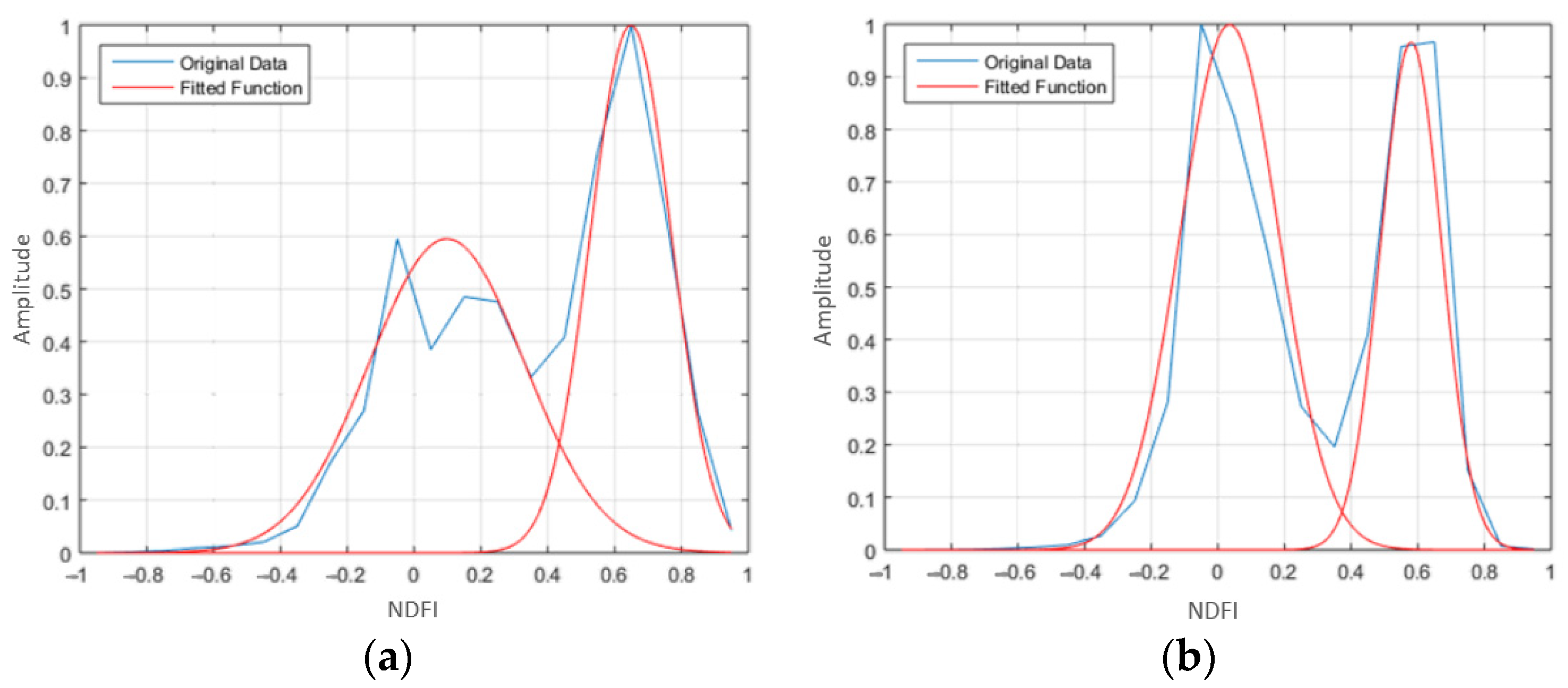
- If the output produced two clusters, the first cluster was buildings or roads class, and the second cluster was trees or grass class.
- If the output produced four clusters, the first two clusters were buildings or roads class, and the last two clusters were trees or grass class.
3.1. The Impact of Spatial Coherence
3.2. Comparison with Previous Studies
4. Conclusions
Author Contributions
Funding
Institutional Review Board Statement
Informed Consent Statement
Data Availability Statement
Acknowledgments
Conflicts of Interest
References
- Yan, W.Y.; Shaker, A.; El-Ashmawy, N. Urban land cover classification using airborne LiDAR data: A review. Remote Sens. Environ. 2015, 158, 295–310. [Google Scholar] [CrossRef]
- Wang, R. 3D building modeling using images and LiDAR: A review. Int. J. Image Data Fusion 2013, 4, 273–292. [Google Scholar] [CrossRef]
- Teo, T.A.; Shih, T.Y. LiDAR-based change detection and change-type determination in urban areas. Int. J. Remote Sens. 2013, 34, 968–981. [Google Scholar] [CrossRef]
- He, M.; Zhu, Q.; Du, Z.; Hu, H.; Ding, Y.; Chen, M. A 3D shape descriptor based on contour clusters for damaged roof detection using airborne LiDAR point clouds. Remote Sens. 2016, 8, 189. [Google Scholar] [CrossRef]
- Axel, C.; van Aardt, J.A. Building damage assessment using airborne LiDAR. J. Appl. Remote Sens. 2017, 11, 046024. [Google Scholar] [CrossRef]
- Matikainen, L.; Pandžić, M.; Li, F.; Karila, K.; Hyyppä, J.; Litkey, P.; Kukko, A.; Lehtomäki, M.; Karjalainen, M.; Puttonen, E. Toward utilizing multitemporal multispectral airborne laser scanning, Sentinel-2, and mobile laser scanning in map updating. J. Appl. Remote Sens. 2019, 13, 044504. [Google Scholar] [CrossRef]
- Chehata, N.; Guo, L.; Mallet, C. Airborne LiDAR feature selection for urban classification using random forests. ISPRS Arch. Photogramm. Remote Sens. Spat. Inf. Sci. 2009, 38, W8. [Google Scholar]
- Mallet, C.; Bretar, F.; Roux, M.; Soergel, U.; Heipke, C. Relevance assessment of full-waveform LiDAR data for urban area classification. ISPRS J. Photogramm. Remote Sens. 2011, 66, S71–S84. [Google Scholar] [CrossRef]
- Xu, S.; Vosselman, G.; Elberink, S.O. Multiple-entity based classification of airborne laser scanning data in urban areas. ISPRS J. Photogramm. Remote Sens. 2014, 88, 1–15. [Google Scholar] [CrossRef]
- Blomley, R.; Jutzi, B.; Weinmann, M. Classification of airborne laser scanning data using geometric multi-scale features and different neighbourhood types. ISPRS Ann. Photogramm. Remote Sens. Spat. Inf. Sci. 2016, 3, 169–176. [Google Scholar] [CrossRef]
- Vosselman, G.; Coenen, M.; Rottensteiner, F. Contextual segment-based classification of airborne laser scanner data. ISPRS J. Photogramm. Remote Sens. 2017, 128, 354–371. [Google Scholar] [CrossRef]
- Niemeyer, J.; Rottensteiner, F.; Soergel, U. Contextual classification of LiDAR data and building object detection in urban areas. ISPRS J. Photogramm. Remote Sens. 2014, 87, 152–165. [Google Scholar] [CrossRef]
- Kokaly, R.F.; Clark, R.N.; Swayze, G.A.; Livo, K.E.; Hoefen, T.M.; Pearson, N.C.; Wise, R.A.; Benzel, W.M.; Lowers, H.A.; Driscoll, R.L.; et al. USGS Spectral Library Version 7: US Geological Survey Data Release; U.S. Geological Survey Data Series; United States Geological Survey (USGS): Reston, VA, USA, 2017; Volume 1035, 61p.
- Fernandez-Diaz, J.C.; Carter, W.; Glennie, C.; Shrestha, R.; Pan, Z.; Ekhtari, N.; Singhania, A.; Hauser, D.; Sartori, M. Capability assessment and performance metrics for the Titan multispectral mapping LiDAR. Remote Sens. 2016, 8, 936. [Google Scholar] [CrossRef]
- Nabucet, J.; Hubert-Moy, L.; Corpetti, T.; Launeau, P.; Lague, D.; Michon, C.; Quénol, H. Evaluation of bispectral LiDAR data for urban vegetation mapping. In Proceedings of the SPIE Remote Sensing Technologies and Applications in Urban Environments, Edinburgh, UK, 26–29 September 2016. [Google Scholar]
- Karila, K.; Matikainen, L.; Puttonen, E.; Hyyppä, J. Feasibility of multispectral airborne laser scanning data for road mapping. IEEE Geosci. Remote Sens. Lett. 2017, 14, 294–298. [Google Scholar] [CrossRef]
- Morsy, S.; Shaker, A.; El-Rabbany, A. Clustering of multispectral airborne laser scanning data using Gaussian decomposition. ISPRS Arch. Photogramm. Remote Sens. Spat. Inf. Sci. 2017, XLII-2/W7, 269–276. [Google Scholar] [CrossRef]
- Morsy, S.; Shaker, A.; El-Rabbany, A. Evaluation of distinctive features for land/water classification from multispectral airborne LiDAR data at Lake Ontario. In Proceedings of the 10th International Conference on Mobile Mapping Technology (MMT), Cairo, Egypt, 6–8 May 2017; pp. 280–286. [Google Scholar]
- Bakuła, K.; Kupidura, P.; Jełowicki, Ł. Testing of land cover classification from multispectral airborne laser scanning data. ISPRS Arch. Photogramm. Remote Sens. Spat. Inf. Sci. 2016, XLI-B7, 161–169. [Google Scholar] [CrossRef]
- Morsy, S.; Shaker, A.; El-Rabbany, A. Potential use of multispectral airborne LiDAR data in land cover classification. In Proceedings of the 37th Asian Conference on Remote Sensing (ACRS), Colombo, Sri Lanka, 17–21 October 2016; p. 296. [Google Scholar]
- Zou, X.; Zhao, G.; Li, J.; Yang, Y.; Fang, Y. 3D land cover classification based on multispectral LiDAR point clouds. ISPRS Arch. Photogramm. Remote Sens. Spat. Inf. Sci. 2016, XLI-B1, 741–747. [Google Scholar] [CrossRef]
- Matikainen, L.; Karila, K.; Hyyppä, J.; Litkey, P.; Puttonen, E.; Ahokas, E. Object-based analysis of multispectral airborne laser scanner data for land cover classification and map updating. ISPRS J. Photogramm. Remote Sens. 2017, 128, 298–313. [Google Scholar] [CrossRef]
- Wichmann, V.; Bremer, M.; Lindenberger, J.; Rutzinger, M.; Georges, C.; Petrini-Monteferri, F. Evaluating the potential of multispectral airborne LiDAR for topographic mapping and land cover classification. ISPRS Ann. Photogramm. Remote Sens. Spat. Inf. Sci. 2015, II-3/W5, 113–119. [Google Scholar] [CrossRef]
- Morsy, S.; Shaker, A.; El-Rabbany, A. Multispectral LiDAR data for land cover classification of urban areas. Sensors 2017, 17, 958. [Google Scholar] [CrossRef]
- Jing, Z.; Guan, H.; Zhao, P.; Li, D.; Yu, Y.; Zang, Y.; Wang, H.; Li, J. Multispectral LiDAR point cloud classification using SE-PointNet++. Remote Sens. 2021, 13, 2516. [Google Scholar] [CrossRef]
- Zhao, P.; Guan, H.; Li, D.; Yu, Y.; Wang, H.; Gao, K.; Junior, J.M.; Li, J. Airborne multispectral LiDAR point cloud classification with a feature Reasoning-based graph convolution network. Int. J. Appl. Earth Obs. Geoinf. 2021, 105, 102634. [Google Scholar] [CrossRef]
- Luo, B.; Yang, J.; Song, S.; Shi, S.; Gong, W.; Wang, A.; Du, L. Target Classification of Similar Spatial Characteristics in Complex Urban Areas by Using Multispectral LiDAR. Remote Sens. 2022, 14, 238. [Google Scholar] [CrossRef]
- Li, D.; Shen, X.; Guan, H.; Yu, Y.; Wang, H.; Zhang, G.; Li, J.; Li, D. AGFP-Net: Attentive geometric feature pyramid network for land cover classification using airborne multispectral LiDAR data. Int. J. Appl. Earth Obs. Geoinf. 2022, 108, 102723. [Google Scholar] [CrossRef]
- Sithole, G.; Vosselman, G. Experimental comparison of filter algorithms for bare-Earth extraction from airborne laser scanning point clouds. ISPRS J. Photogramm. Remote Sens. 2004, 59, 85–101. [Google Scholar] [CrossRef]
- Dehnad, K. Density Estimation for Statistics and Data Analysis. Technometrics 1987, 29, 495. [Google Scholar] [CrossRef]
- Wagner, W.; Ullrich, A.; Ducic, V.; Melzer, T.; Studnicka, N. Gaussian decomposition and calibration of a novel small-footprint full-waveform digitising airborne laser scanner. ISPRS J. Photogramm. Remote Sens. 2006, 60, 100–112. [Google Scholar] [CrossRef]
- Mallet, C.; Bretar, F. Full-waveform topographic LiDAR: State-of-the-art. ISPRS J. Photogramm. Remote Sens. 2009, 64, 1–16. [Google Scholar] [CrossRef]
- Hofton, M.A.; Minster, J.B.; Blair, J.B. Decomposition of laser altimeter waveforms. IEEE Trans. Geosci. Remote Sens. 2000, 38, 1989–1996. [Google Scholar] [CrossRef]
- Persson, Å.; Söderman, U.; Töpel, J.; Ahlberg, S. Visualization and analysis of full-waveform airborne laser scanner data. ISPRS Arch. Photogramm. Remote Sens. Spat. Inf. Sci. 2005, 36, 103–108. [Google Scholar]
- Charaniya, A.P.; Manduchi, R.; Lodha, S.K. Supervised parametric classification of aerial LiDAR data. In Proceedings of the IEEE Computer Society Conference on Computer Vision and Pattern Recognition Workshops, Washington, DC, USA, 27 June–2 July 2004. [Google Scholar]
- Lodha, S.K.; Fitzpatrick, D.M.; Helmbold, D.P. Aerial LiDAR data classification using expectation-maximization. In Proceedings of the SPIE Conference on Vision Geometry XV, San Jose, CA, USA, 28 January–1 February 2007; pp. 177–187. [Google Scholar]
- Jutzi, B.; Stilla, U. Range determination with waveform recording laser systems using a Wiener Filter. ISPRS J. Photogramm. Remote Sens. 2006, 61, 95–107. [Google Scholar] [CrossRef]
- Dempster, A.P.; Laird, N.M.; Rubin, D.B. Maximum likelihood from incomplete data via the EM algorithm. J. R. Stat. Soc. Ser. B 1977, 39, 1–22. [Google Scholar]
- Oliver, J.J.; Baxter, R.A.; Wallace, C.S. Unsupervised learning using MML. In Proceedings of the 13th International Conference on Machine Learning (ICML), Bari, Italy, 3–6 July 1996; pp. 364–372. [Google Scholar]
- Chauve, A.; Mallet, C.; Bretar, F.; Durrieu, S.; Deseilligny, M.P.; Puech, W. Processing full-waveform LiDAR data: Modelling raw signals. In Proceedings of the ISPRS Workshop Laser Scanning and SilviLaser (LS SL), Espoo, Finland, 12–14 September 2007; pp. 102–107. [Google Scholar]
- Chen, Y.; Su, W.; Li, J.; Sun, Z. Hierarchical object oriented classification using very high resolution imagery and LiDAR data over urban areas. Adv. Space Res. 2009, 43, 1101–1110. [Google Scholar] [CrossRef]
- Hartfield, K.A.; Landau, K.I.; Van Leeuwen, W.J. Fusion of high resolution aerial multispectral and LiDAR data: Land cover in the context of urban mosquito habitat. Remote Sens. 2011, 3, 2364–2383. [Google Scholar] [CrossRef]
- Singh, K.K.; Vogler, J.B.; Shoemaker, D.A.; Meentemeyer, R.K. LiDAR-Landsat data fusion for large-area assessment of urban land cover: Balancing spatial resolution, data volume and mapping accuracy. ISPRS J. Photogramm. Remote Sens. 2012, 74, 110–121. [Google Scholar] [CrossRef]


| Class | IC1 | IC2 | IC3 | NDFIC2−C1 | NDFIC2−C3 | NDFIC1−C3 |
|---|---|---|---|---|---|---|
| Red Trees | I | I | 0 | V | 1 | 1 |
| Power lines | I | 0 | 0 | −1 | NAN | 1 |
| Swimming pools | 0 | 0 | I | NAN | −1 | −1 |
| Parameter | Specification | |
|---|---|---|
| Area 1 | Area 2 | |
| Dimension (m × m) | 600 × 410 | 490 × 470 |
| Altitude (m) | ~1075 | |
| Scan Angle | ±20° | |
| Pulse Repetition Frequency (PRF) | 200 kHz/channel; 600 kHz total | |
| Scan Frequency | 40 Hz | |
| Number of Returns | Up to 4 returns | |
| Number of points: Channel 1 Channel 2 Channel 3 | 833,216 | 796,226 |
| 887,744 | 825,176 | |
| 723,102 | 742,158 | |
| Average Point Spacing (m) | 0.51/channel | |
| Class | Area 1 | Area 2 |
|---|---|---|
| Buildings | 10,398 | 10,234 |
| Green Trees | 7140 | 7453 |
| Red Trees | 2506 | 4472 |
| Roads | 4078 | 5734 |
| Grass | 8792 | 9013 |
| Swimming Pools | 538 | 1289 |
| Total | 33,452 | 38,195 |
| NDFIC2−C1 | NDFIC2−C3 | NDFIC1−C3 | MVGD | ||
|---|---|---|---|---|---|
| Area 1 | Aboveground | 0.051 | 0.048 | 0.042 | 4 |
| Ground | 0.033 | 0.040 | 0.082 | 4 | |
| Area 2 | Aboveground | 0.079 | 0.062 | 0.065 | 2 |
| Ground | 0.032 | 0.097 | 0.092 | 4 |
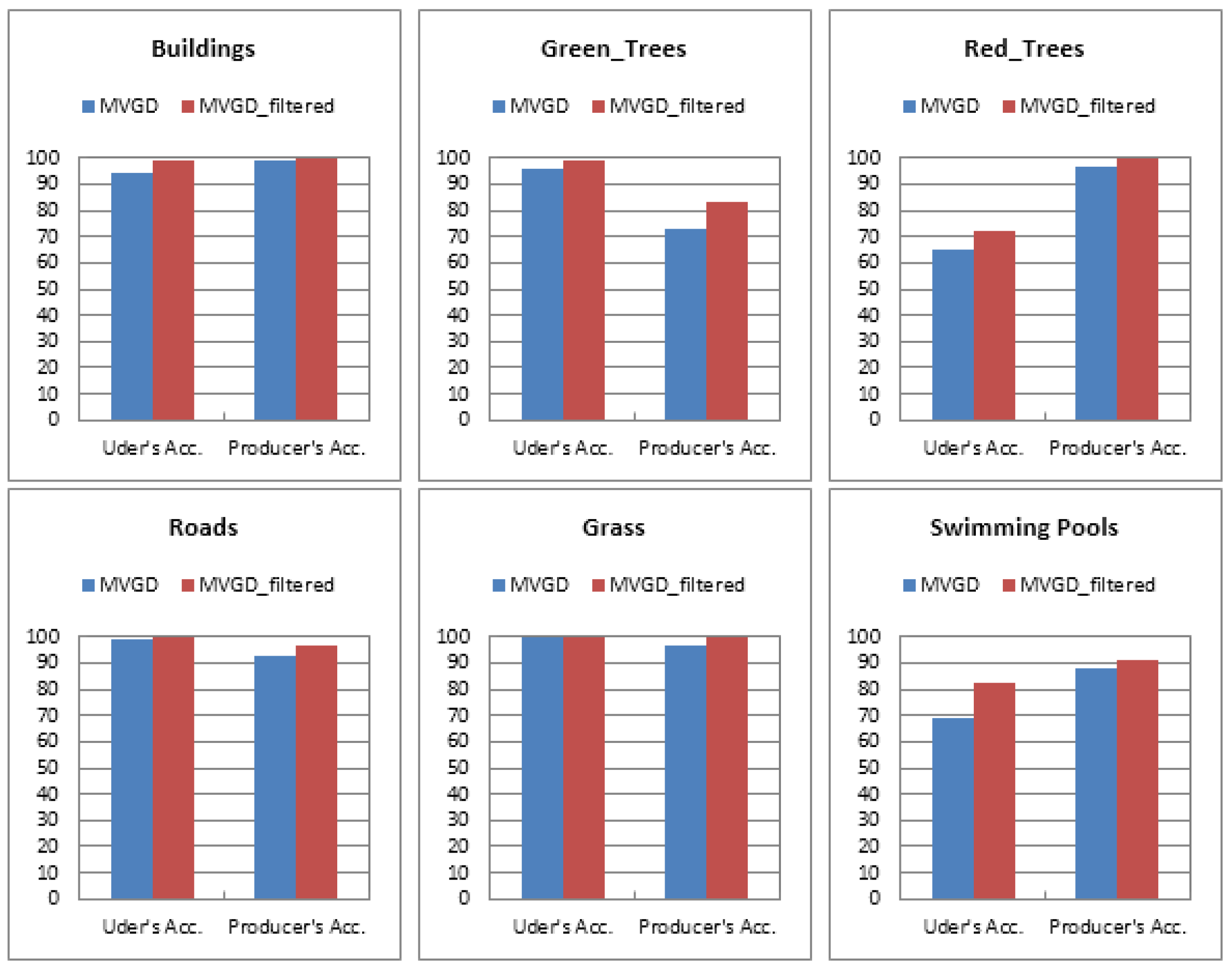
| Class | Producer’s Accuracy (%) | User’s Accuracy (%) |
|---|---|---|
| Buildings | 99.0 | 94.2 |
| Green Trees | 72.8 | 96.2 |
| Red Trees | 96.6 | 64.7 |
| Roads | 92.5 | 98.8 |
| Grass | 97.0 | 99.9 |
| Swimming Pools | 88.1 | 69.4 |
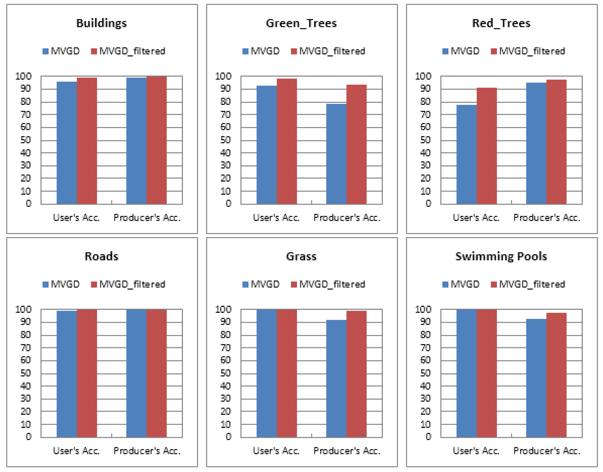
| Class | Producer’s Accuracy (%) | User’s Accuracy (%) |
|---|---|---|
| Buildings | 99.1 | 95.7 |
| Green Trees | 78.9 | 92.5 |
| Red Trees | 95.5 | 77.5 |
| Roads | 99.7 | 98.9 |
| Grass | 92.2 | 99.9 |
| Swimming Pools | 93.0 | 99.7 |
Publisher’s Note: MDPI stays neutral with regard to jurisdictional claims in published maps and institutional affiliations. |
© 2022 by the authors. Licensee MDPI, Basel, Switzerland. This article is an open access article distributed under the terms and conditions of the Creative Commons Attribution (CC BY) license (https://creativecommons.org/licenses/by/4.0/).
Share and Cite
Morsy, S.; Shaker, A.; El-Rabbany, A. Classification of Multispectral Airborne LiDAR Data Using Geometric and Radiometric Information. Geomatics 2022, 2, 370-389. https://doi.org/10.3390/geomatics2030021
Morsy S, Shaker A, El-Rabbany A. Classification of Multispectral Airborne LiDAR Data Using Geometric and Radiometric Information. Geomatics. 2022; 2(3):370-389. https://doi.org/10.3390/geomatics2030021
Chicago/Turabian StyleMorsy, Salem, Ahmed Shaker, and Ahmed El-Rabbany. 2022. "Classification of Multispectral Airborne LiDAR Data Using Geometric and Radiometric Information" Geomatics 2, no. 3: 370-389. https://doi.org/10.3390/geomatics2030021
APA StyleMorsy, S., Shaker, A., & El-Rabbany, A. (2022). Classification of Multispectral Airborne LiDAR Data Using Geometric and Radiometric Information. Geomatics, 2(3), 370-389. https://doi.org/10.3390/geomatics2030021