Article

Classification of Multispectral Airborne LiDAR Data Using Geometric and Radiometric Information

1
Public Works Department, Faculty of Engineering, Cairo University, 1 El Gamaa Street, Giza 12613, Egypt
2
Department of Civil Engineering, Toronto Metropolitan University, 350 Victoria Street, Toronto, ON M5B 2K3, Canada
*
Author to whom correspondence should be addressed.
Geomatics 2022, 2(3), 370-389; https://doi.org/10.3390/geomatics2030021
Submission received: 28 June 2022 / Revised: 5 September 2022 / Accepted: 6 September 2022 / Published: 9 September 2022

Abstract

:
Classification of airborne light detection and ranging (LiDAR) point cloud is still challenging due to the irregular point cloud distribution, relatively low point density, and the complex urban scenes being observed. The availability of multispectral LiDAR systems allows for acquiring data at different wavelengths with a variety of spectral information from land objects. In this research, a rule-based point classification method of three levels for multispectral airborne LiDAR data covering urban areas is presented. The first level includes ground filtering, which attempts to distinguish aboveground from ground points. The second level aims to divide the aboveground and ground points into buildings, trees, roads, or grass using three spectral indices, namely normalized difference feature indices (NDFIs). A multivariate Gaussian decomposition is then used to divide the NDFIs’ histograms into the aforementioned four classes. The third level aims to label more classes based on their spectral information such as power lines, types of trees, and swimming pools. Two data subsets were tested, which represent different complexity of urban scenes in Oshawa, Ontario, Canada. It is shown that the proposed method achieved an overall accuracy up to 93%, which is increased to over 98% by considering the spatial coherence of the point cloud.

1. Introduction

Over the past two decades, airborne light detection and ranging (LiDAR) data have been widely used in classification of urban scenes [1]. In 3D point cloud classification of airborne LiDAR data, multi-class labeling has become the norm for city modeling, land change detection, map updating, emergency purposes, and disaster evaluation [2,3,4,5,6]. Multispectral airborne LiDAR data are currently gaining interest due to their diversity of spectral information collected along with spatial attributes.
Previously, most studies focused on the geometric characteristics described by the LiDAR data [7,8,9,10,11]. Blomley et al. [10] extracted geometric features from the LiDAR point cloud based on multiple scales and different neighborhood types. Then, random forest (RF) classifier was applied to classify the terrain into ground, buildings, cars, trees, and low vegetation. A standard benchmark dataset was used for evaluations. The results of five classes, namely ground, building, cars, trees, and low vegetation, demonstrated an overall accuracy of 76.8% and 86.6% for two data subsets. Vosselman et al. [11] proposed a contextual segment-based classification using conditional random field (CRF) for LiDAR point cloud classification. A combination between different point cloud segmentation methods was used to avoid under- and over-segmentation. The results demonstrated that the overall accuracy of seven classes in a 30 points/m2 dataset was 91.2%, compared to 82.8% obtained from point-based classification using CRF. Other studies were reported on the use of LiDAR intensity data along with geometric features for the purpose of urban scenes classification. Niemeyer et al. [12] applied contextual classification on airborne full waveform LiDAR data by integrating an RF classifier with a CRF framework. A total of 36 features were extracted from the LiDAR data to accomplish this classification process. An overall accuracy of 83.4% was achieved when the LiDAR data were classified into grassland, road, buildings with gabled roofs, low vegetation, façades, buildings with flat roofs, and trees. Although the presented method was applied on points and no segmentation was performed, it is computationally expensive due to the huge number of features extracted. Moreover, reports were confirmed of confusion between a number of classes such as trees and façades as well as trees and gable roofs. The reason for this confusion is that the data were collected during leaf-on conditions, when trees partially cover roofs and façades. Moreover, confusion between low vegetation, trees and grassland was reported and this is attributed to the generation of reference data, which was very difficult for a human operator. That study showed the importance of using the LiDAR intensity in distinguishing grassland from road. Thus, intensity should not be eliminated by the feature importance selection and should be included for all cases. It is the goal of this research to present a classification method of urban areas from only airborne LiDAR data, which provide spectral information, without using image data.
The first commercial multispectral airborne LiDAR system, namely Optech Titan, was launched by Teledyne Optech in 2014. This system operates at three wavelengths of 1550 nm, 1064 nm, and 532 nm in three channels C1, C2, and C3 with looking angles of 3.5° forward, 0° nadir, and 7° forward, respectively. Multispectral information for 3D point cloud is simultaneously available for the first time from one system. Figure 1 shows the spectral reflectance curve of different objects at the three channels. These curves were drawn from the USGS Spectral Digital Library [13]. C3 wavelength penetrates water bodies and is reflected, while C1 and C2 wavelengths are completely absorbed by clear calm water. Using the green wavelength at C3 ensures high density point cloud for shallow water mapping. Vegetation (e.g., grass and trees) is strongly reflective at the near infrared (NIR) wavelength from C2, while soil (e.g., clay) is more reflective than vegetation at the C3 and C1 wavelengths. As such, combining multispectral LiDAR data collected with the aforementioned three wavelengths ensures a higher reliability and accuracy of information extraction compared to monochromatic wavelength LiDAR systems. In addition, this system can be used for topographic mapping, vegetation mapping, and 3D land cover classification.
Over the past six years, investigations have been conducted to analyze the Optech Titan’s multispectral information and to explore its capability for different applications such as land cover classification, measuring water depths in shallow water areas, and mapping forests [14]. Some of these investigations focused on one application such as vegetation mapping [15] and road mapping [16]. Other studies extracted more than one object such as separation of high and low vegetation from built-up areas [17] and land/water discrimination [18].
The multispectral LiDAR point cloud data, collected by the Titan system, have been used for land cover classification by converting those point cloud data into images [19,20,21,22]. Morsy et al. [20] showed that the accuracy of land cover classification can be significantly improved when multispectral LiDAR data are used, as opposed to single intensity data. They first created intensity images and digital surface model (DSM) from the collected point cloud at each wavelength. After that, they applied maximum likelihood algorithm as classification technique to each single intensity image, the fused intensity images (from C1, C2, and C3), and the fused intensity images with the DSM, in order to classify terrain into buildings, trees, roads, grass, soil, and wetland. The use of a single intensity LiDAR image, created from each of the C1, C2, and C3, led to overall classification accuracies of 34.0%, 48.5%, and 41.5%, respectively. The overall classification accuracy was improved to 65.5% using the fused three-intensity images. Moreover, the overall classification accuracy was increased to 72.5% by incorporating the height LiDAR data (i.e., DSM image). Matikainen et al. [22] presented an object-based analysis of multispectral LiDAR data, whereas intensity images from the three channels, maximum DSM, minimum DSM, and DTM were first generated. Subsequently, those images were segmented, and then 41 features based on intensity and height from the three channels were calculated for each segment. The segments were divided into high and low based on their mean height with a threshold value of 2.5 m. Training segments for high objects (i.e., buildings and trees) and low objects (i.e., asphalt, gravel, rocky areas and low vegetation) were selected from high and low segments, respectively. The training segments were used as input for RF classifier in order to investigate the importance of using the 41 features for classification. The classification results of a suburban area demonstrated an overall accuracy of 95.9%. The aforementioned studies focused on image data classification. These images vary according to the selected pixel size and the interpolation methods used to fill the gaps between pixels. In addition, the occurrence of mixed pixels is a fundamental problem in those studies. Moreover, supervised classification methods that require prior knowledge/training areas of the obtained classes were used.
With the focus on LiDAR point cloud classification, Wichmann et al. [23] used classification and mapping procedures in order to classify the multispectral LiDAR data. In addition, the spectral patterns of different classes were studied and showed that the multispectral data could potentially be used in land cover classification. Morsy et al. [24] developed a point-based classification method to label the 3D multispectral LiDAR points. A ground filtering method was first applied in order to separate ground from aboveground points. Three pseudo normalized difference vegetation indices (NDVIs) were then computed based on the three channels combination for aboveground and ground points. Subsequently, the Jenks natural break optimization method was used to classify aboveground and ground points into trees or buildings and grass or roads. This method demonstrated an overall accuracy of up to 92.7%. A combination utilization of the three NDVIs could maximize the usefulness of multispectral LiDAR data as well as increase the number of extracted classes.
Recently, many studies have been carried out using machine learning (ML) and deep learning (DL) classifiers. For instance, Jing et al. [25] applied a point-based classification architecture using an improved PointNet++ semantic segmentation considering Squeeze-and-Excitation (SE) block. The SE-PointNet++ architecture achieved an overall accuracy and Kappa coefficient of 91.2% and 0.86, respectively. Zhao et al. [26] applied a feature reasoning-based graph convolution network that achieved an overall accuracy of 93.6%. Similar to [20], Luo et al. [27] classified the multispectral LiDAR point cloud instead of images using a single-channel and three-channel data. A ground filtering was first applied, then a decision tree was conducted on the combination of spatial and spectral information. An improvement of the overall accuracy from 64.7% to 93.8% was achieved considering the three intensity channels. Li et al. [28] applied a DL-based method named attentive graph geometric moments convolution (AGGM Convolution). In that method, multi-scale geometric features were extracted and fused. The AGGM Convolution achieved an overall accuracy and Kappa coefficient of 96.9% and 0.95, respectively. Using either ML or DL classifiers achieve promising performance in multispectral airborne LiDAR point clouds classification. However, they require a massive training data to learn the classifier. In addition, DL classifiers are more computationally complex.
With the emerging of multispectral airborne LiDAR systems in the market, the point density has been increased with a variety of spectral information recorded from land covers. Assigning each 3D point to an object class is a basic step in LiDAR processing for land cover classification. The classification of airborne LiDAR point cloud in urban areas have become challenging due to (1) the availability of dense point cloud requiring automatic, efficient, and low computational costs processing algorithms; (2) objects that are hardly detectable in urban areas such as swimming pools and power lines due to the lack of data collected for such objects—this problem is caused either by occlusion or no points being recorded at certain wavelengths; and (3) complex urban scenes such as vegetation covering building roofs and power lines that can be confused from elevated objects (mostly vegetation).
To overcome these challenges, a rule-based classification method from multispectral airborne LiDAR data is presented in this research. The LiDAR point from the three channels are first merged, followed by the application of a ground filtering method. Two data subsets of an urban area with different characteristics are tested. The first is a clear separation between vegetation and built-up areas (e.g., buildings and roads). The second is a mixed scene of buildings, trees, roads, grass, swimming pools, and power lines. The contributions of this research include: (1) Multi-class labelling (i.e., seven classes) from 3D LiDAR point cloud directly; (2) the application of multivariate Gaussian decomposition (MVGD) combined with the interpretation of spectral information of the multispectral LiDAR data in the classification process; and (3) the consideration of spatial coherence of the point cloud in improving the classification results. In this research, we maximize the utilization of multispectral LiDAR data for urban scenes classification.

2. Materials and Methods

2.1. Overall Classification Scheme

The goal of this research is to assign each LiDAR point a unique label. The overall classification scheme is shown in Figure 2. The LiDAR point cloud acquired at the three channels were first combined in a pre-processing step, followed by a rule-based classification on three levels. The first level relied on ground filtering, whereas aboveground points were separated from ground points based on elevation. The second level was based on spectral information (i.e., intensity values), whereas the recorded intensity values were used to compute three spectral indices, namely normalized difference feature indices (NDFIs), followed by NDFIs’ histograms construction for ground and aboveground points. The multivariate Gaussian decomposition (MVGD) was then used to analyze the NDFIs’ histograms into different Gaussian components to classify the LiDAR points into buildings, trees, roads, or grass. The third level relied on the interpretation of the interaction between objects at the three wavelengths, whereas returns from a certain channel were recorded for an object, while no returns were recorded for the same object from a different channel such as swimming pools, power lines, and trees with red leaves. Consequently, the LiDAR data were eventually classified into eight classes, namely buildings, trees with green leaves (green trees), trees with red leaves (red trees), roads, grass, swimming pools, power lines and unclassified points. The classification results were finally evaluated using aerial images and accuracy measures were calculated.

2.1.1. LiDAR Points Merging and Ground Filtering

The multispectral sensor acquires LiDAR point cloud in three channels (C1, C2, and C3) at different wavelengths with different intensity values. However, merging those point cloud and estimating the intensity values for each single point at all wavelengths make the available data denser and more reliable. In order to estimate intensity values for each LiDAR point, a median value of a point was calculated from its neighboring points from another channel [24]. The median values were used to avoid any outliers in the dataset. Let pi, pj, and ph represent points in C1, C2, and C3, respectively; where i = 1, 2, 3,…, n1; j = 1, 2, 3,…, n2; h = 1, 2, 3,…, n3; and n1, n2 and n3 are the total number of LiDAR points collected in C1, C2, and C3, respectively. For any point pi in C1, the neighboring points from C2 and C3 were obtained within a sphere of predefined search radius r. Then, the median intensity values IC2 and IC3 were estimated using the neighboring points from C2 and C3, respectively. Similarly, for any point pj in C2, the neighboring points from C1 and C3 were obtained and the intensity values IC1 and IC3 were estimated. The same was applied for each point ph in C3, where the intensity values IC1 and IC2 were estimated using the neighboring points from C1 and C2, respectively. Finally, the total number of points N = n1 + n2 + n3 (with duplicated points removed), and each LiDAR point had attributes of x, y, z, IC1, IC2 and IC3; where IC1 is the intensity value from C1, IC2 is the intensity value from C2, and IC3 is the intensity value from C3. During the merging process, for a point in C1, if no neighboring points were found in C2 or C3, the intensity value of this point was set to zero. Thus, a LiDAR point could have zero intensity values from one or two channels. Although this is not a practical situation, it is useful for labeling certain classes (e.g., power lines) as detailed in Section 2.1.4.
The classification method started with distinguishing between aboveground and ground points. A slope-based ground filtering method was applied to achieve this task [29]. The slope of each point with respect to its neighboring points was calculated and a threshold value (S_thrd) was applied. If the slope of a LiDAR point was greater than S_thrd, this point was labeled as aboveground points. Moreover, a moving circle of radius r and relying on a height difference threshold value (H_thrd) was applied to ensure that all aboveground and ground were correctly labeled.

2.1.2. NDFIs Computation and Histograms Construction

For aboveground and ground points, the three intensity values IC1, IC2, and IC3 were employed to form three NDFIs, namely NDFIC2−C1, NDFIC2−C3, and NDFIC1−C3, which were defined in [17] as follows:
N D F I C 2 C 1 = I C 2 I C 1 I C 2 + I C 1
N D F I C 2 C 3 = I C 2 I C 3 I C 2 + I C 3
N D F I C 1 C 3 = I C 1 I C 3 I C 1 + I C 3
The NDFIs values, similar to spectral indices, range from −1 to 1. It should be noted that if a point was assigned with zero intensity value in two channels, the NDFI resulted in NaN. Consequently, the point was assigned to the unclassified class.
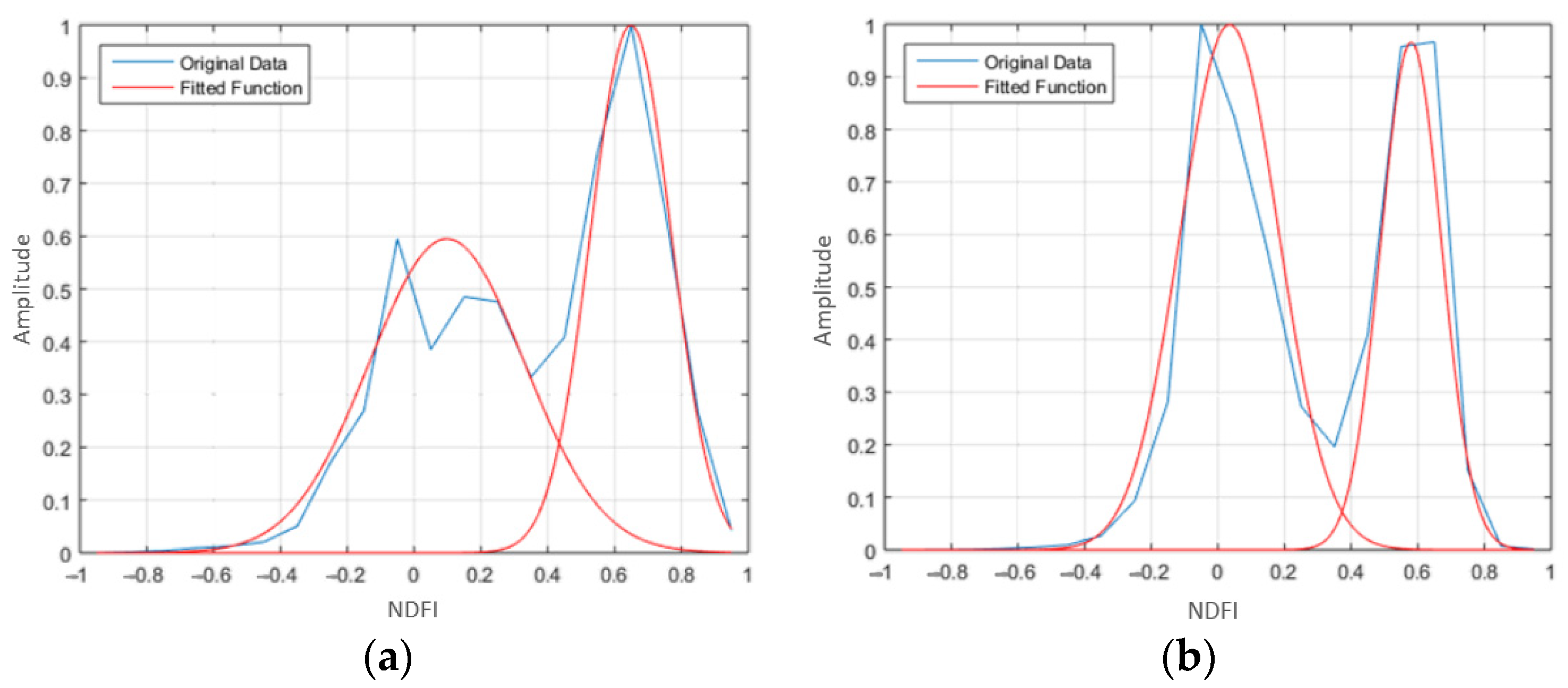
A histogram is the graphical representation of the distribution of any data. The histogram has been used to create intensity histograms by plotting the number of pixels for each digital number in an image [30]. Similarly, in this research, NDFI values were divided into bins (or intervals) and the number of points were counted (i.e., frequency) in each bin. The NDFIs’ histograms were then constructed. Figure 3 shows examples of NDFIs’ histograms and fitted functions.

2.1.3. MVGD Application

Multivariate Gaussian decomposition is based on the Gaussian function in Equation (4). It has been used for modeling LiDAR data, especially full-waveform LiDAR [31]. Gaussian decompression requires a fitting algorithm [32] such as non-linear least-squares approach [31,33] and maximum likelihood estimate using Levenberg–Marquardt optimization algorithm and expectation-maximization (EM) algorithm [34], respectively. Apart from the full waveform LiDAR data, Gaussian decomposition was used to model training samples for supervised classification of discrete returns LiDAR data [35,36]. In this research, we used the Gaussian function to model the NDFIs’ histograms. A sum of Gaussian functions G(x), described by [34], was applied to model each NDFI’s histogram as defined by:
f ( x ) = 1 2 π σ j 2 e x p ( ( x μ j ) 2 2 σ j 2 )
where,
  • μ j : the mean value
  • σ j : the standard deviation
G ( x ) = j = 1 N p j   .   f j ( x )
where,
  • x: the bin value
  • N: the number of components
  • p j : the relative weight
Two main challenges were identified related to the fitting of the modeling function (i.e., Gaussian). First, a prior knowledge of the number of Gaussian components was required. Second, the fitting was sensitive to initial values of Gaussian’s parameters. Therefore, we applied the peak detection algorithm to locate all peaks (K) in each histogram [37]. Usually, the Gaussian component has two inflection points. The positions of those inflection points can be estimated using the zero crossing of the second derivative. Based on those locations the Gaussian’s half width ( σ j ) was estimated [33].
To model the histograms, the number of Gaussian components was considered equal to the number of peaks (N = K). Then, the p j , μ j , and σ j parameters were fitted for each Gaussian component using the maximum likelihood estimate produced by EM algorithm [38], starting with two Gaussians that have equal relative weight ( p j ), as shown in Equation (6).
f w i j = p j     f j ( x i ) j = 1 N p j     f j ( x i )
where wij is the probability of xi belongs to Gaussian (j). The maximization (M) step computes the maximum likelihood estimates of the parameters (pj, µj, and σj) as follows:
p j = i = 1 n y i   w i j i = 1 n y i
μ j = i = 1 n y i   w i j p j   i = 1 n y i
σ j = i = 1 n y i   w i j   ( x i μ j ) 2 p j   i = 1 n y i
where
  • y i : the amplitude at bin xi
  • n: the number of histogram’s bins
The two steps were repeated until convergence or a maximum number of iterations was achieved. The process stopped when either (1) the difference between any iteration and the previous iteration was less than 0.001, or (2) the number of iterations was greater than 1000 [39]. The same procedures were repeated for all possible numbers of Gaussians, where N = K − 1, K − 2, …, 2. In addition, a non-linear least squares (NLS) adjustment was utilized to optimize each component’s parameters ( μ j and σ j ) [31,33], so that they could be compared with the fitted Gaussians from EM, as shown in Figure 3.
The quality of the fitted Gaussians has been tested for fitting the full waveform LiDAR data [33,40] using the following formula:
ξ = 1 n i = 1 n ( y i f ( x i ) ) 2
Similarly, the fitted Gaussians was tested using the quality Equation (10). According to [40], a good fitting is considered when ξ is less than a threshold value (i.e., 0.5). However, in this research, in each case from N = K, K − 1,, 1;  ξ was calculated. Then, the number of Gaussian components were considered with minimal ξ . A MVGD was finally used to classify the LiDAR point cloud as follows:
f M V G ( x ) = 1 2 π m / 2 | | 1 / 2 e x p ( 1 2 ( X M ) T 1   ( X M ) )
  • m: number of variables (NDFIC2−C1, NDFIC2−C3, and NDFIC1−C3)
  • X: variables matrix [NDFIC2−C1 NDFIC2−C3 NDFIC1−C3]
  • M: means row vector
  • Σ: covariance matrix

2.1.4. LiDAR Points Classification

Eight classes were labeled from the airborne multispectral LiDAR data, namely buildings, green trees, red trees, roads, grass, swimming pools, power lines, and unclassified points. Vegetation (i.e., trees or grass) exhibits different reflectance values in the three channels, whereas reflectance from C2 > C1 > C3 as shown in Figure 1. As a result, the calculated NDFIs of the vegetation points exhibited higher values than the built-up areas (i.e., buildings or roads). Thus, the output clusters from MVGD that have high NDFIs were labeled as “vegetation” and those with low NDFIs were labeled as “built-up areas”.
After the ground filtering was applied as described in Section 2.1.1, the application of MVGD clustered the aboveground points into trees and buildings, and the ground points into grass and roads. Moreover, for the aboveground points, the trees class was separated into two classes: green trees and red trees. The red trees had no reflectance in C3 (532 nm), as shown in Figure 4. As a result, for a point belonging to red trees, IC3 = 0 and hence the NDFIC2−C3 = NDFIC1−C3 = 1. In addition, power lines had reflectance mainly in C1 (1550 nm), which is sensitive to the high temperature emitted from the power lines, as shown in Figure 5. That means, for power lines points, IC2IC3 ≈ 0, and hence NDFIC2−C1 = −1 and NDFIC1−C3 = 1. Similarly, swimming pool points were labeled based on the fact that they had returns mainly in C3. Therefore, for swimming pool points, IC1IC2 ≈ 0, and hence NDFIC2−C3 = −1 and NDFIC1−C3 = −1. Table 1 summarizes the expected intensity values and the NDFIs values calculated from Equations (1)–(3) of points belonging to red trees, power lines, and swimming pools. As aforementioned, if a point had zero intensity value in any two channels, this point was labeled as an unclassified point unless it was a point belonging to power lines or swimming pools.
The proposed point-based classification approach labels each individual point according to its spectral characteristics and its position in the feature space. In general, the point-based classification methods are full of salt and pepper noises, as they do not account for spatial coherence of neighborhoods. As a result, the derived labeling was expected to be noisy. Therefore, a spatial coherence was considered with applied a max voting 3D filter similarly to the one presented by [35]. Each individual point was assigned to a class that occurs most frequently in its neighborhood within a circle of a 3 m radius. This filter provided smooth classification results as shown in Figure 6.

2.1.5. Classification Results Evaluation

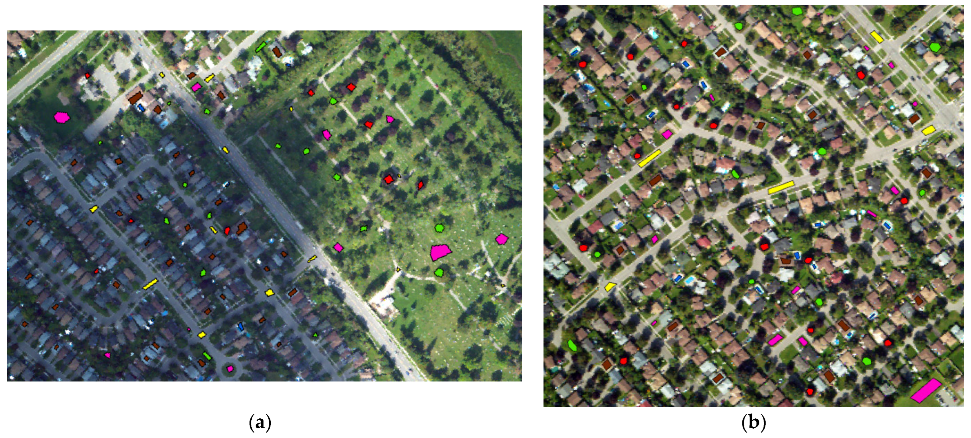
Previous studies used 3D-labeled LiDAR data benchmarks [10,11] or 2D-labeled LiDAR data benchmarks that were extended to 3D-labeled points [12], which are not available for the tested study area. This research presented an alternative method for generating 3D reference points based on polygons digitized from aerial images. First, a set of polygons for each class (e.g., buildings) were randomly selected for different classes and manually digitized from aerial images. Second, all 3D points within each polygon were labeled as reference points for their class. Third, the same polygons were intersected with the classified points, and all points within the polygons were used (classified points) in computing the confusion matrix (reference points vs classified points). This method is applicable for buildings, roads, grass, and swimming pools classes. For trees class, only the canopy points were labeled as reference points. This is because we can only see the canopy from aerial images, and we are not able to see what is underneath. In addition, other classes (e.g., power lines) could not be quantitatively assessed as they are vertically distributed in the LiDAR data and appeared as linear objects in the aerial images (see Figure 6); moreover, reference polygons cannot be digitized. The confusion matrix for each data subset was computed and the accuracy measures (overall, producer’s and user’s accuracies) were calculated.

2.2. Study Area and Datasets

The performance of our method was evaluated using LiDAR data acquired by the Optech Titan multispectral airborne LiDAR sensor for a strip over Oshawa, Ontario, Canada in September 2014. Two data subsets from the LiDAR strip were clipped for experimental testing. The two subsets are described as follows. Area 1 is divided into two parts: mixed built-up with vegetation and vegetation area. It also includes power lines and a number of swimming pools. Area 2 is a mixed area between built-up and vegetation consisting of residential and industrial buildings with different roof materials (colors), road surfaces, high and low vegetation, power lines and swimming pools. Table 2 summarizes the specifications the two data subsets.
Since the data acquisition was in summertime during leaf-on conditions, most points of the vertical distribution within trees describe the canopy only. The variation in the number of points recorded at different channels depends on the interaction of land objects with different wavelengths (e.g., reflection from the water surface and/or bottom, and greenness of the vegetation). The lowest number of points is in C3 because there are no recorded returns from the trees with red leaves in this channel. Figure 7 shows two aerial images of the tested areas. The aerial images were geo-referenced with the LiDAR data with 0.5 m pixel size. The reference points that were used for validating the land cover classification results as listed in Table 3.

3. Results and Discussion

The LiDAR data from the three Titan channels were first merged, and a ground filtering method was applied. The ground filtering method relied on points’ slopes with respect to surrounding points, whereas a threshold value (S_thrd = 10°) was applied to label an aboveground point. Moreover, the remaining points were filtered by a moving circle of (r = 10 m). The point was labeled as an aboveground point, if the height difference was greater than 1 m (H_thrd = 1 m).
The three NDFIs were then calculated, and NDFIs’ histograms were constructed with 0.1 bin size and normalized for aboveground and ground points. As aforementioned, Gaussian distributions with minimum ξ was utilized to fit the histograms. The ξ values are listed in Table 4.
As shown in Table 3, the max ξ is less than 0.1 which is lower than the prescribed error level (i.e., 0.5) by [40]. The fitted Gaussians with their parameters ( μ j and σ j ) were used as input for the multivariate Gaussian function, (Equation (11)), in order to cluster aboveground/ground points into four classes. For the three defined NDFIs of the aboveground or ground points, the lower values represent buildings or roads, and the higher values represent trees or grass as reported in [24]. Based on these facts and based on a visual interpretation of the output clusters, the following decisions were applied:
  • If the output produced two clusters, the first cluster was buildings or roads class, and the second cluster was trees or grass class.
  • If the output produced four clusters, the first two clusters were buildings or roads class, and the last two clusters were trees or grass class.
Consequently, the MVGD divided the multispectral airborne LiDAR data into four main classes: trees, buildings, grass, and roads. The number of classes could be increased, if we considered more Gaussian components and allowed a higher error level of ξ ; however, in this case the output classes might be noisy and not representative.
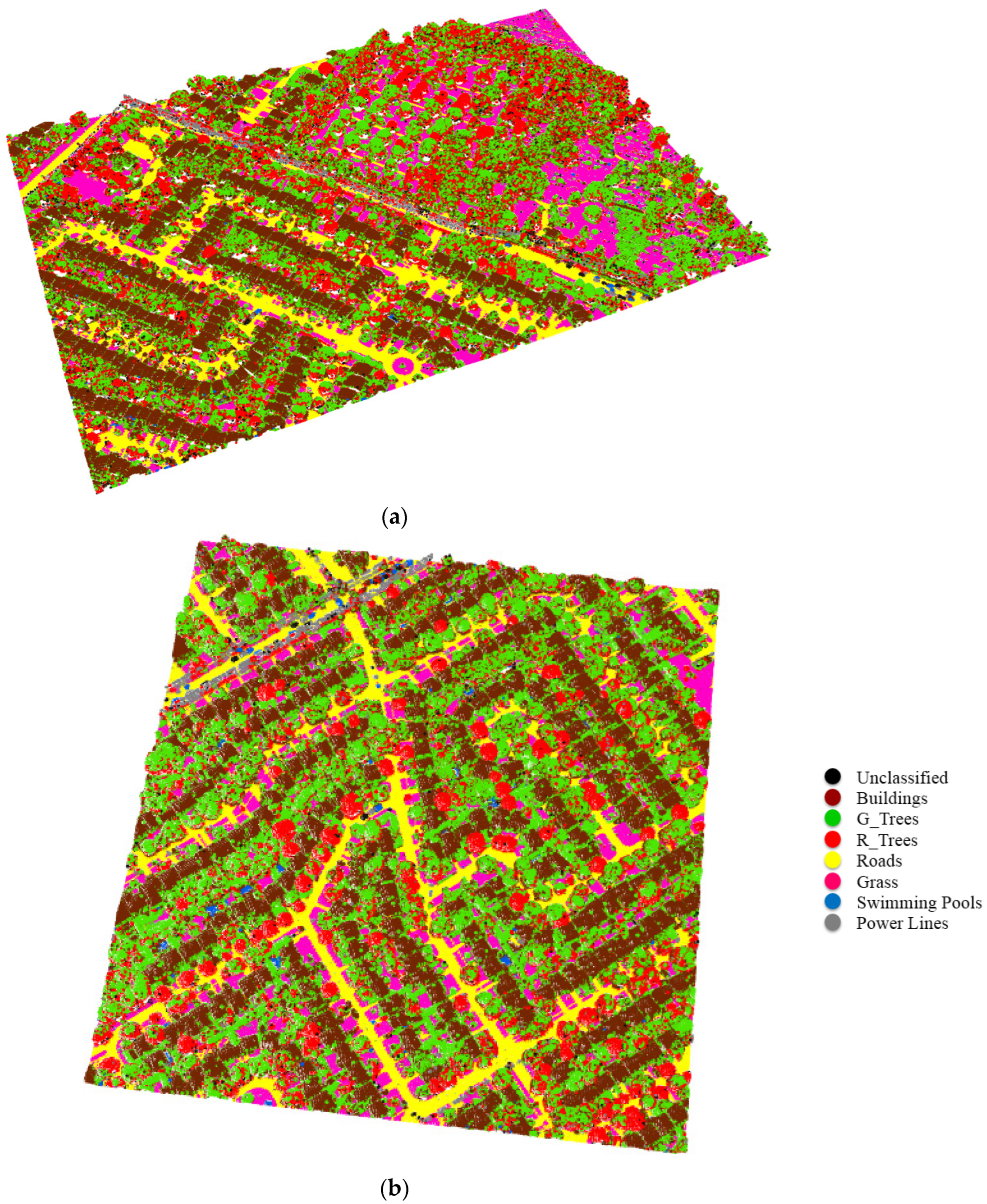
In addition, more classes were labeled based on the spectral information of land objects produced by the three different wavelengths. First, the trees class was separated into two classes: green trees and red trees. Moreover, power lines, swimming pools and unclassified points were labeled. As a result, a total of eight classes were labeled, including buildings, green trees, red trees, roads, grass, power lines swimming pools, and unclassified objects. Figure 8 shows the classified point cloud of Area 1 and Area 2. Table 5 and Table 6 provide the producer’s and user’s accuracies of Area 1 and Area 2, respectively.
Our method achieved an overall accuracy of 91.7% and 93.0% for Area 1 and Area 2, respectively. The main sources of the classification errors are the unclassified class and ground filtering. The error of unclassified class ranges from 1.1% to 1.7%. The classification errors due to the ground filtering ranged from 0.0% to 3.7%, whereas the ground points were misclassified as aboveground points or vice versa.
The confusion between green trees and red trees is another source of the classification errors. This is attributed to the fact that intensity values along the vertical distribution of the tree profile are not the same as they represent different returns. For example, in Area 2, about 21.1% of green trees points were omitted (78.9% producer’s accuracy), and those points were classified as red trees or buildings. This omission caused a classification error rate of red trees class of about 17.5% and of buildings of about 3.9%. As vegetation cover increased, the error rate increased. About 27.2% (72.8% producer accuracy) and 29.9% (71.1% producer accuracy) of green trees points were omitted in Area 1 and Area 2, respectively. In some cases, the tree points were wrongly classified as buildings or vice versa. This is primarily due to the various moisture content of the high vegetation (trees)/low vegetation (grass) and various roof materials that exhibit different intensity values as reported by the results in [24].
Swimming pools have a relatively low user accuracy of 69.4% in Area 1 due to a number of roads and grass points being incorrectly assigned to this class. This occurred because no returns were recorded in one or more channels for those points. Power line points were visually assessed and most of these points were correctly labeled in Area 2 but not in Area 1. The misclassified points were labeled as trees or unclassified objects. This is due to those points had returns from two/three channels (labeled as trees) or returns in one channel, either C2 or C3 (labeled as unclassified).

3.1. The Impact of Spatial Coherence

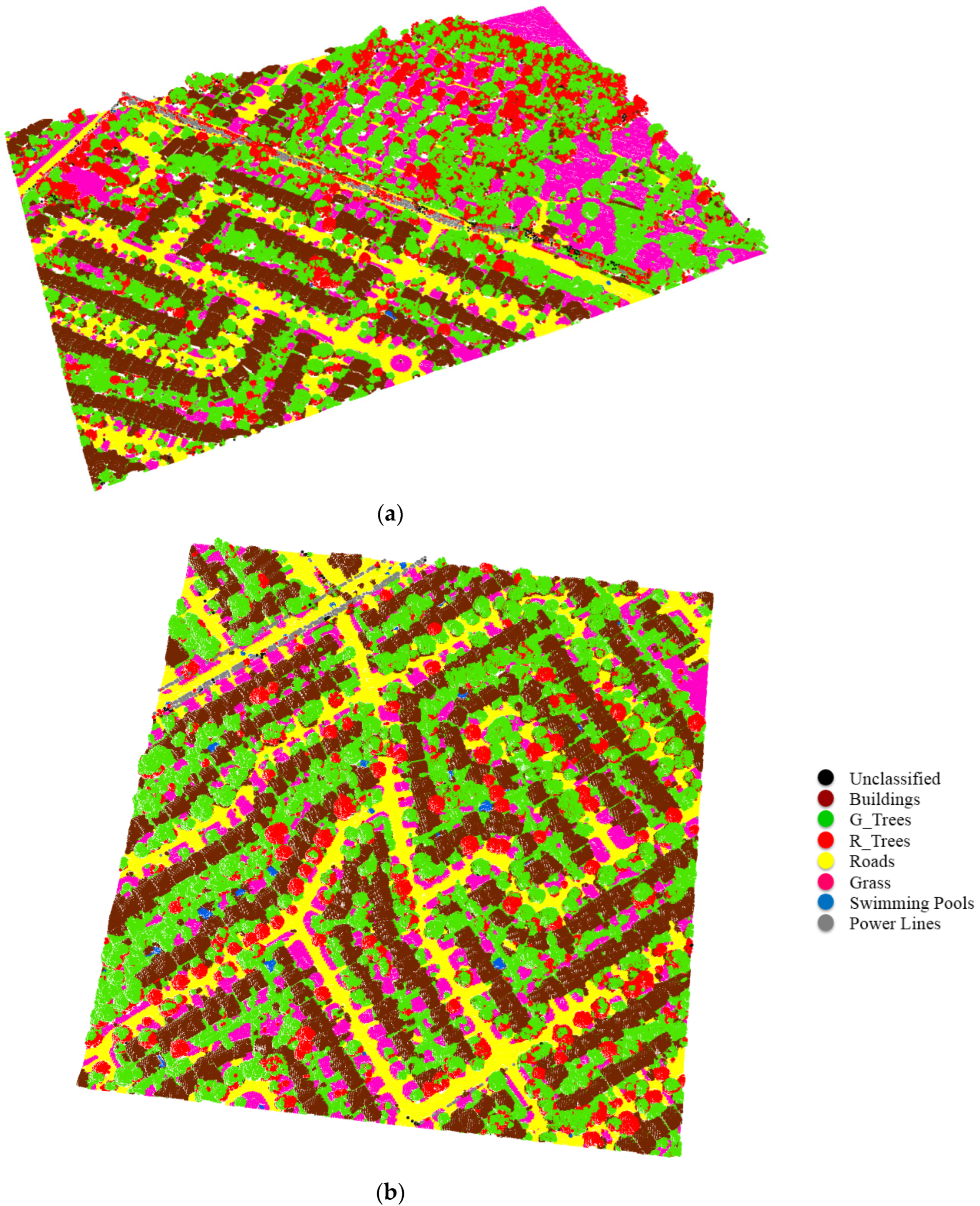
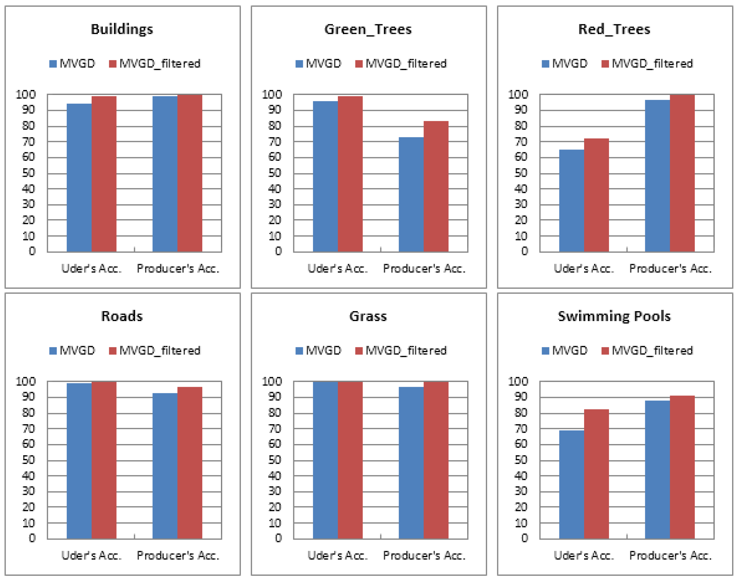
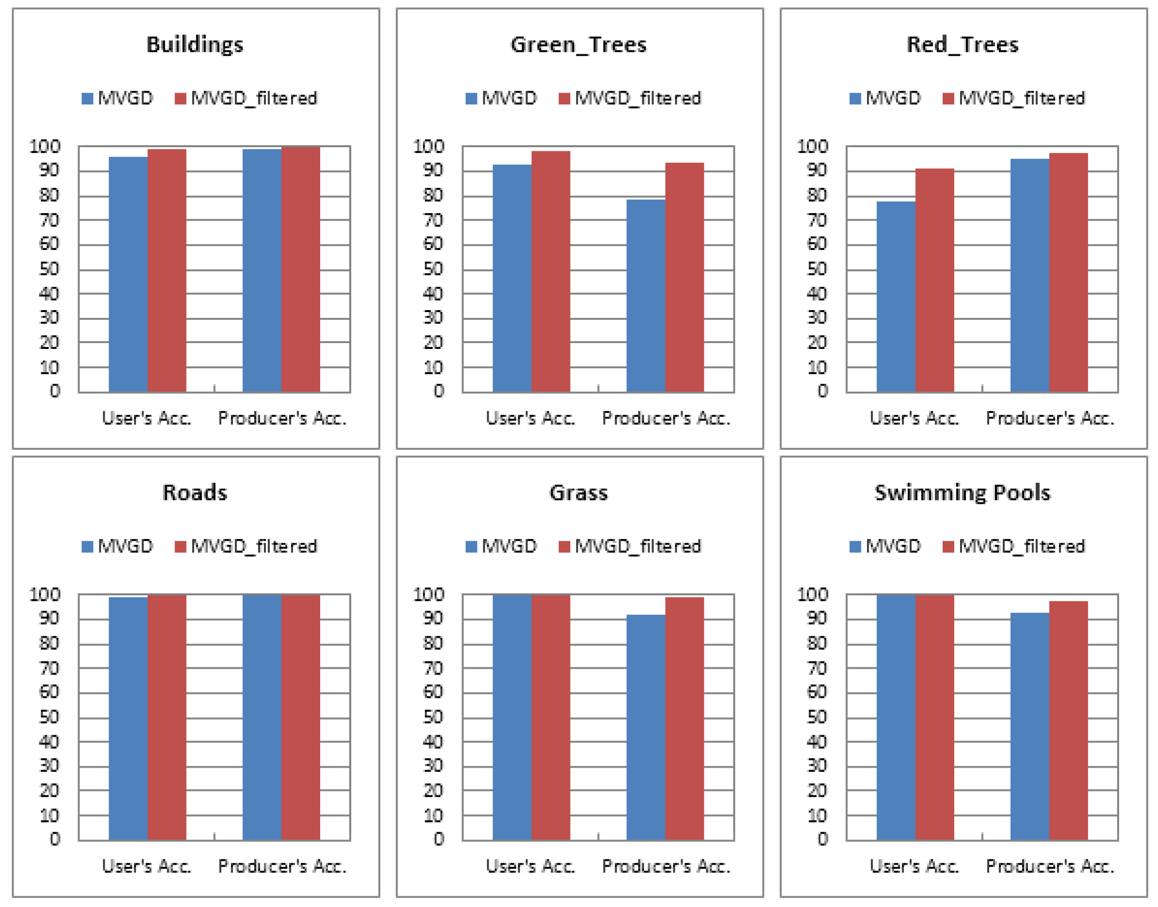
In order to improve the classification results, a 3D max voting (mode) filter with a circle of 3 m radius was applied to the classification output classes. The overall accuracies increased to 95.7% and 98.3% for Area 1 and Area 2, respectively. Figure 9 shows the classified point cloud of the two areas after the application of the 3D filter. Significant improvements of the accuracy measures were achieved after the application of the 3D filter (MVGD_filtered) as shown in Figure 10 and Figure 11. For instant, the user’s accuracy in classifying buildings, red trees, and swimming pools improved by up to 22.7%, 13.9%, and 13.3%, respectively. Moreover, the producer’s accuracy improved from 10.2–18.6% and from 4.5–13.3% for green trees and swimming pools, respectively.

3.2. Comparison with Previous Studies

The achieved classification results have proven the usefulness of multispectral LiDAR data for land cover classification. Previous studies combined multispectral aerial images and/or satellite imagery with either LiDAR height [41] or with both LiDAR height and intensity [42,43] in order to classify the terrain into multi-class. Those studies demonstrated classification accuracies between 85.4% and 89.9%, while our method achieved a higher score of 97.0% average overall accuracy. Thus, the availability of the multispectral LiDAR data reduces the need for multispectral aerial/satellite imagery for classification purposes. In contrast, by focusing on classifying LiDAR points into multi-class in urban areas, previous studies achieved overall classification accuracies of 89.1% [9], 83.4% [12], or 82.8% [11]. In addition, the results of recent that applied ML/DL classifiers demonstrated overall classification accuracies of 91.2% [25], 93.6% [26], 93.8% [27], or 96.9% [28]. The classification results in this research demonstrated higher overall accuracies compared to the aforementioned studies.
For a quantitative comparison, we applied the same clustering method presented in [24]. The Jenks natural breaks optimization method was used to cluster the three NDFIs (NDFIC2−C1, NDFIC2−C3, and NDFIC1−C3) histograms of the aboveground and ground points into buildings or trees and roads or grass, respectively. The same method was applied to the two datasets presented in this research. Figure 12 shows the overall accuracies achieved from the three NDFIs based on Jenks break optimization, MVGD, and MVGD after applying the 3D filter (MVD_filtered) for the four classes. The utilization of MVGD achieved overall accuracies similar to or higher than NDFIs based on Jenks breaks for the tested areas. In addition, the application of the 3D filter (MVGD_filtered) demonstrated the highest overall accuracies for the two tested areas.

4. Conclusions

In this research, a rule-based point classification method from multispectral airborne LiDAR point cloud covering an urban area was presented. The capability of using geometric and radiometric information of the LiDAR data in land cover classification was demonstrated. The airborne multispectral LiDAR sensor, Optech Titan, was used to acquire point cloud in three channels at different wavelengths (1550 nm, 1064 nm, and 532 nm). The LiDAR data were first merged and intensity values for each LiDAR point were estimated in a pre-processing step. A ground filtering method was applied to separate aboveground from ground points. Three NDFIs were then calculated and NDFIs’ histograms were constructed. The NDFIs’ histograms were fitted using a Gaussian decomposition with EM and NLS. The output Gaussian parameters were used as an input to MVGD, whereas four main classes (buildings, trees, roads, and grass) were automatically clustered from the multispectral LiDAR data. The data acquisition at different wavelengths from land objects allowed for labeling additional classes based on their spectral information. Thus, swimming pools, power lines and two types of trees were classified. Two data subsets collected from an urban area were used for evaluation. The data subsets represented different complexities of urban scenes. The presented approach revealed an average overall accuracy of 92.4%. Moreover, the spatial coherence of the LiDAR point cloud was considered by using a max voting 3D filter, where the average overall accuracy improved to 97.0%.
The ground filtering method showed high potential in separation, whereas the slope of aboveground LiDAR points was considered. The results revealed the usefulness of NDFIs in distinguishing between high and low vegetation and built-up areas with an overall accuracy of more than 95.0%. In addition, the spatial coherence consideration for the classified LiDAR points achieved a significant improvement in the obtained overall accuracies. However, we found that the trees with green leaves and trees with red leaves are most confusing and caused classification errors. Moreover, the different building roof materials caused misclassification with vegetation. Many points of the power lines were visually evaluated and many points were labeled as either trees or unclassified points.
Future work will focus on radiometric correction and normalization of the multispectral data that could improve the classification accuracy of misclassified objects. In addition, more land objects such as buildings with different roof materials, bare soil, and road markings will be considered in the classification process.

Author Contributions

Conceptualization, S.M., A.S. and A.E.-R.; methodology, S.M., A.S. and A.E.-R.; software, S.M.; validation, S.M.; formal analysis, S.M.; investigation, S.M.; resources, A.S.; data curation, S.M.; writing—original draft preparation, S.M.; writing—review and editing, A.S. and A.E.-R.; visualization, S.M.; supervision, A.S. and A.E.-R.; project administration, A.S. and A.E.-R.; funding acquisition, S.M., A.S. and A.E.-R. All authors have read and agreed to the published version of the manuscript.

Funding

This research work was funded by Discovery Grant from the Natural Sciences and Engineering Research Council of Canada (NSERC) and the Ontario Trillium Scholarship (OTS).

Institutional Review Board Statement

Not applicable.

Informed Consent Statement

Not applicable.

Data Availability Statement

Not applicable.

Acknowledgments

The authors would like to thank Paul E. LaRocque from Teledyne Optech for providing the LiDAR data from the world’s first commercial multispectral airborne LiDAR system, Optech Titan.

Conflicts of Interest

The authors declare no conflict of interest.

References

  1. Yan, W.Y.; Shaker, A.; El-Ashmawy, N. Urban land cover classification using airborne LiDAR data: A review. Remote Sens. Environ. 2015, 158, 295–310. [Google Scholar] [CrossRef]
  2. Wang, R. 3D building modeling using images and LiDAR: A review. Int. J. Image Data Fusion 2013, 4, 273–292. [Google Scholar] [CrossRef]
  3. Teo, T.A.; Shih, T.Y. LiDAR-based change detection and change-type determination in urban areas. Int. J. Remote Sens. 2013, 34, 968–981. [Google Scholar] [CrossRef]
  4. He, M.; Zhu, Q.; Du, Z.; Hu, H.; Ding, Y.; Chen, M. A 3D shape descriptor based on contour clusters for damaged roof detection using airborne LiDAR point clouds. Remote Sens. 2016, 8, 189. [Google Scholar] [CrossRef]
  5. Axel, C.; van Aardt, J.A. Building damage assessment using airborne LiDAR. J. Appl. Remote Sens. 2017, 11, 046024. [Google Scholar] [CrossRef]
  6. Matikainen, L.; Pandžić, M.; Li, F.; Karila, K.; Hyyppä, J.; Litkey, P.; Kukko, A.; Lehtomäki, M.; Karjalainen, M.; Puttonen, E. Toward utilizing multitemporal multispectral airborne laser scanning, Sentinel-2, and mobile laser scanning in map updating. J. Appl. Remote Sens. 2019, 13, 044504. [Google Scholar] [CrossRef]
  7. Chehata, N.; Guo, L.; Mallet, C. Airborne LiDAR feature selection for urban classification using random forests. ISPRS Arch. Photogramm. Remote Sens. Spat. Inf. Sci. 2009, 38, W8. [Google Scholar]
  8. Mallet, C.; Bretar, F.; Roux, M.; Soergel, U.; Heipke, C. Relevance assessment of full-waveform LiDAR data for urban area classification. ISPRS J. Photogramm. Remote Sens. 2011, 66, S71–S84. [Google Scholar] [CrossRef]
  9. Xu, S.; Vosselman, G.; Elberink, S.O. Multiple-entity based classification of airborne laser scanning data in urban areas. ISPRS J. Photogramm. Remote Sens. 2014, 88, 1–15. [Google Scholar] [CrossRef]
  10. Blomley, R.; Jutzi, B.; Weinmann, M. Classification of airborne laser scanning data using geometric multi-scale features and different neighbourhood types. ISPRS Ann. Photogramm. Remote Sens. Spat. Inf. Sci. 2016, 3, 169–176. [Google Scholar] [CrossRef]
  11. Vosselman, G.; Coenen, M.; Rottensteiner, F. Contextual segment-based classification of airborne laser scanner data. ISPRS J. Photogramm. Remote Sens. 2017, 128, 354–371. [Google Scholar] [CrossRef]
  12. Niemeyer, J.; Rottensteiner, F.; Soergel, U. Contextual classification of LiDAR data and building object detection in urban areas. ISPRS J. Photogramm. Remote Sens. 2014, 87, 152–165. [Google Scholar] [CrossRef]
  13. Kokaly, R.F.; Clark, R.N.; Swayze, G.A.; Livo, K.E.; Hoefen, T.M.; Pearson, N.C.; Wise, R.A.; Benzel, W.M.; Lowers, H.A.; Driscoll, R.L.; et al. USGS Spectral Library Version 7: US Geological Survey Data Release; U.S. Geological Survey Data Series; United States Geological Survey (USGS): Reston, VA, USA, 2017; Volume 1035, 61p.
  14. Fernandez-Diaz, J.C.; Carter, W.; Glennie, C.; Shrestha, R.; Pan, Z.; Ekhtari, N.; Singhania, A.; Hauser, D.; Sartori, M. Capability assessment and performance metrics for the Titan multispectral mapping LiDAR. Remote Sens. 2016, 8, 936. [Google Scholar] [CrossRef]
  15. Nabucet, J.; Hubert-Moy, L.; Corpetti, T.; Launeau, P.; Lague, D.; Michon, C.; Quénol, H. Evaluation of bispectral LiDAR data for urban vegetation mapping. In Proceedings of the SPIE Remote Sensing Technologies and Applications in Urban Environments, Edinburgh, UK, 26–29 September 2016. [Google Scholar]
  16. Karila, K.; Matikainen, L.; Puttonen, E.; Hyyppä, J. Feasibility of multispectral airborne laser scanning data for road mapping. IEEE Geosci. Remote Sens. Lett. 2017, 14, 294–298. [Google Scholar] [CrossRef]
  17. Morsy, S.; Shaker, A.; El-Rabbany, A. Clustering of multispectral airborne laser scanning data using Gaussian decomposition. ISPRS Arch. Photogramm. Remote Sens. Spat. Inf. Sci. 2017, XLII-2/W7, 269–276. [Google Scholar] [CrossRef]
  18. Morsy, S.; Shaker, A.; El-Rabbany, A. Evaluation of distinctive features for land/water classification from multispectral airborne LiDAR data at Lake Ontario. In Proceedings of the 10th International Conference on Mobile Mapping Technology (MMT), Cairo, Egypt, 6–8 May 2017; pp. 280–286. [Google Scholar]
  19. Bakuła, K.; Kupidura, P.; Jełowicki, Ł. Testing of land cover classification from multispectral airborne laser scanning data. ISPRS Arch. Photogramm. Remote Sens. Spat. Inf. Sci. 2016, XLI-B7, 161–169. [Google Scholar] [CrossRef]
  20. Morsy, S.; Shaker, A.; El-Rabbany, A. Potential use of multispectral airborne LiDAR data in land cover classification. In Proceedings of the 37th Asian Conference on Remote Sensing (ACRS), Colombo, Sri Lanka, 17–21 October 2016; p. 296. [Google Scholar]
  21. Zou, X.; Zhao, G.; Li, J.; Yang, Y.; Fang, Y. 3D land cover classification based on multispectral LiDAR point clouds. ISPRS Arch. Photogramm. Remote Sens. Spat. Inf. Sci. 2016, XLI-B1, 741–747. [Google Scholar] [CrossRef]
  22. Matikainen, L.; Karila, K.; Hyyppä, J.; Litkey, P.; Puttonen, E.; Ahokas, E. Object-based analysis of multispectral airborne laser scanner data for land cover classification and map updating. ISPRS J. Photogramm. Remote Sens. 2017, 128, 298–313. [Google Scholar] [CrossRef]
  23. Wichmann, V.; Bremer, M.; Lindenberger, J.; Rutzinger, M.; Georges, C.; Petrini-Monteferri, F. Evaluating the potential of multispectral airborne LiDAR for topographic mapping and land cover classification. ISPRS Ann. Photogramm. Remote Sens. Spat. Inf. Sci. 2015, II-3/W5, 113–119. [Google Scholar] [CrossRef]
  24. Morsy, S.; Shaker, A.; El-Rabbany, A. Multispectral LiDAR data for land cover classification of urban areas. Sensors 2017, 17, 958. [Google Scholar] [CrossRef]
  25. Jing, Z.; Guan, H.; Zhao, P.; Li, D.; Yu, Y.; Zang, Y.; Wang, H.; Li, J. Multispectral LiDAR point cloud classification using SE-PointNet++. Remote Sens. 2021, 13, 2516. [Google Scholar] [CrossRef]
  26. Zhao, P.; Guan, H.; Li, D.; Yu, Y.; Wang, H.; Gao, K.; Junior, J.M.; Li, J. Airborne multispectral LiDAR point cloud classification with a feature Reasoning-based graph convolution network. Int. J. Appl. Earth Obs. Geoinf. 2021, 105, 102634. [Google Scholar] [CrossRef]
  27. Luo, B.; Yang, J.; Song, S.; Shi, S.; Gong, W.; Wang, A.; Du, L. Target Classification of Similar Spatial Characteristics in Complex Urban Areas by Using Multispectral LiDAR. Remote Sens. 2022, 14, 238. [Google Scholar] [CrossRef]
  28. Li, D.; Shen, X.; Guan, H.; Yu, Y.; Wang, H.; Zhang, G.; Li, J.; Li, D. AGFP-Net: Attentive geometric feature pyramid network for land cover classification using airborne multispectral LiDAR data. Int. J. Appl. Earth Obs. Geoinf. 2022, 108, 102723. [Google Scholar] [CrossRef]
  29. Sithole, G.; Vosselman, G. Experimental comparison of filter algorithms for bare-Earth extraction from airborne laser scanning point clouds. ISPRS J. Photogramm. Remote Sens. 2004, 59, 85–101. [Google Scholar] [CrossRef]
  30. Dehnad, K. Density Estimation for Statistics and Data Analysis. Technometrics 1987, 29, 495. [Google Scholar] [CrossRef]
  31. Wagner, W.; Ullrich, A.; Ducic, V.; Melzer, T.; Studnicka, N. Gaussian decomposition and calibration of a novel small-footprint full-waveform digitising airborne laser scanner. ISPRS J. Photogramm. Remote Sens. 2006, 60, 100–112. [Google Scholar] [CrossRef]
  32. Mallet, C.; Bretar, F. Full-waveform topographic LiDAR: State-of-the-art. ISPRS J. Photogramm. Remote Sens. 2009, 64, 1–16. [Google Scholar] [CrossRef]
  33. Hofton, M.A.; Minster, J.B.; Blair, J.B. Decomposition of laser altimeter waveforms. IEEE Trans. Geosci. Remote Sens. 2000, 38, 1989–1996. [Google Scholar] [CrossRef]
  34. Persson, Å.; Söderman, U.; Töpel, J.; Ahlberg, S. Visualization and analysis of full-waveform airborne laser scanner data. ISPRS Arch. Photogramm. Remote Sens. Spat. Inf. Sci. 2005, 36, 103–108. [Google Scholar]
  35. Charaniya, A.P.; Manduchi, R.; Lodha, S.K. Supervised parametric classification of aerial LiDAR data. In Proceedings of the IEEE Computer Society Conference on Computer Vision and Pattern Recognition Workshops, Washington, DC, USA, 27 June–2 July 2004. [Google Scholar]
  36. Lodha, S.K.; Fitzpatrick, D.M.; Helmbold, D.P. Aerial LiDAR data classification using expectation-maximization. In Proceedings of the SPIE Conference on Vision Geometry XV, San Jose, CA, USA, 28 January–1 February 2007; pp. 177–187. [Google Scholar]
  37. Jutzi, B.; Stilla, U. Range determination with waveform recording laser systems using a Wiener Filter. ISPRS J. Photogramm. Remote Sens. 2006, 61, 95–107. [Google Scholar] [CrossRef]
  38. Dempster, A.P.; Laird, N.M.; Rubin, D.B. Maximum likelihood from incomplete data via the EM algorithm. J. R. Stat. Soc. Ser. B 1977, 39, 1–22. [Google Scholar]
  39. Oliver, J.J.; Baxter, R.A.; Wallace, C.S. Unsupervised learning using MML. In Proceedings of the 13th International Conference on Machine Learning (ICML), Bari, Italy, 3–6 July 1996; pp. 364–372. [Google Scholar]
  40. Chauve, A.; Mallet, C.; Bretar, F.; Durrieu, S.; Deseilligny, M.P.; Puech, W. Processing full-waveform LiDAR data: Modelling raw signals. In Proceedings of the ISPRS Workshop Laser Scanning and SilviLaser (LS SL), Espoo, Finland, 12–14 September 2007; pp. 102–107. [Google Scholar]
  41. Chen, Y.; Su, W.; Li, J.; Sun, Z. Hierarchical object oriented classification using very high resolution imagery and LiDAR data over urban areas. Adv. Space Res. 2009, 43, 1101–1110. [Google Scholar] [CrossRef]
  42. Hartfield, K.A.; Landau, K.I.; Van Leeuwen, W.J. Fusion of high resolution aerial multispectral and LiDAR data: Land cover in the context of urban mosquito habitat. Remote Sens. 2011, 3, 2364–2383. [Google Scholar] [CrossRef]
  43. Singh, K.K.; Vogler, J.B.; Shoemaker, D.A.; Meentemeyer, R.K. LiDAR-Landsat data fusion for large-area assessment of urban land cover: Balancing spatial resolution, data volume and mapping accuracy. ISPRS J. Photogramm. Remote Sens. 2012, 74, 110–121. [Google Scholar] [CrossRef]
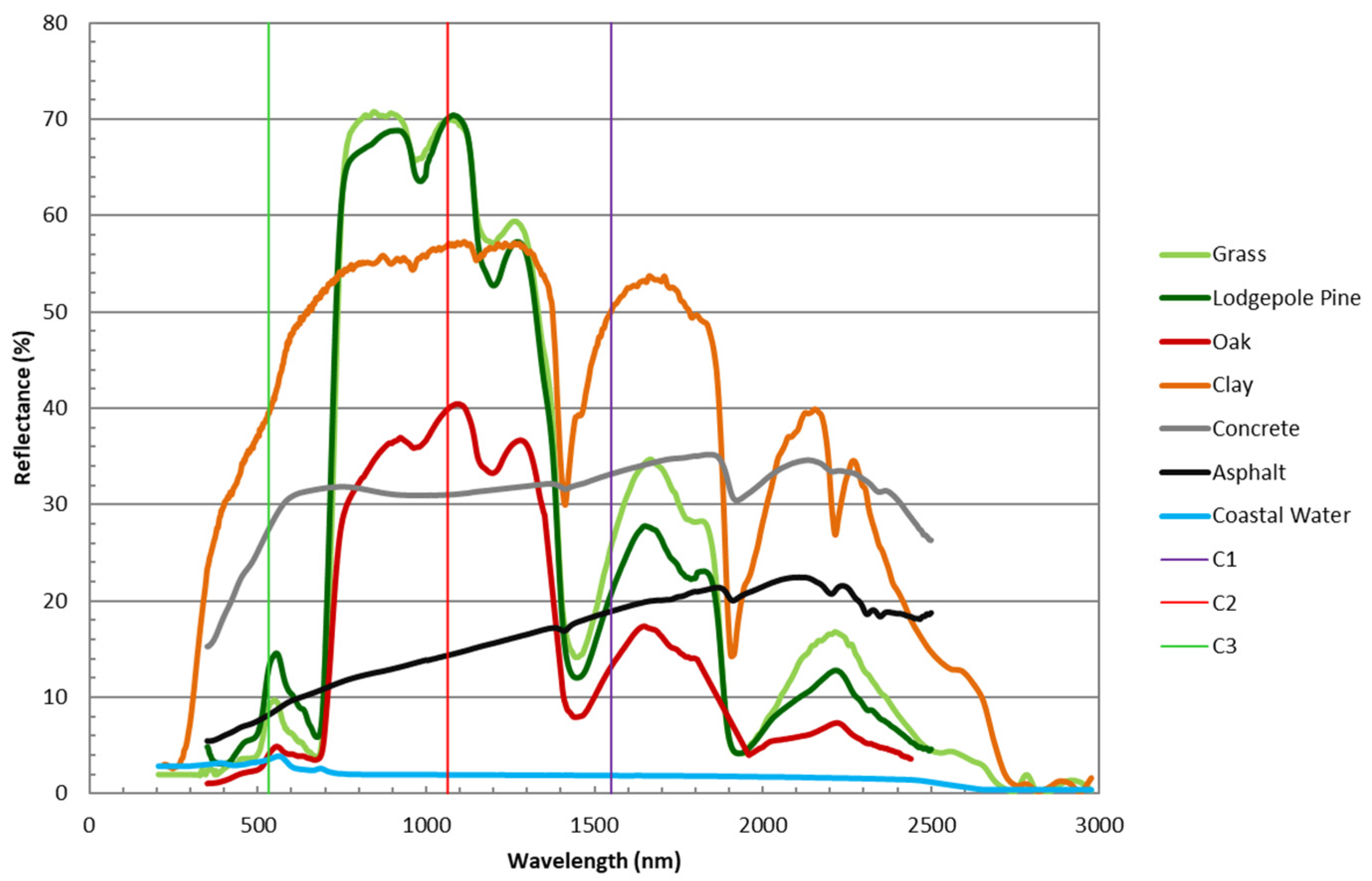
Figure 1. Spectral reflectance curve of different land covers at different wavelengths, including C1 (1550 nm), C2 (1064 nm), and C3 (532 nm).
Geomatics 02 00021 g001
Figure 2. Classification workflow.
Geomatics 02 00021 g002
Figure 3. Examples of NDFIs’ histograms of: (a) aboveground points; (b) ground points.
Geomatics 02 00021 g003
Figure 4. Display of LiDAR point cloud of two types of trees colored by elevation showing that the trees with red leaves do not have returns in C3, but have returns in C1 and C2: (a) aerial image; (b) LiDAR point cloud in C1; (c) LiDAR point cloud in C2; (d) LiDAR point cloud in C3. Trees with red leaves are marked by red in (a) and black in (bd).
Geomatics 02 00021 g004
Figure 5. Display of LiDAR point cloud of power lines colored by elevation showing that the power lines have more returns in C3 than in C2 and C1: (a) street view of the power lines; (b) LiDAR point cloud in C1; (c) LiDAR point cloud in C2; (d) LiDAR point cloud in C3.
Geomatics 02 00021 g005
Figure 6. Classified point cloud showing the improvement of using the 3D filter: (a) aerial image; (b) classified point cloud before the application of the 3D filter; (c) classified point cloud after the application of the 3D filter.
Geomatics 02 00021 g006
Figure 7. Aerial images of the tested datasets with reference polygons: (a) Area 1; (b) Area 2. Buildings (brown), trees with green leaves (green), trees with red leaves (red), roads (yellow), grass (pink), and swimming pools (blue).
Geomatics 02 00021 g007
Figure 8. Classified LiDAR point cloud of: (a) Area 1; (b) Area 2. Corresponding RGB images are shown in Figure 7.
Geomatics 02 00021 g008
Figure 9. Classified LiDAR points after the application of the 3D filter of: (a) Area 1; (b) Area 2. Corresponding RGB images are shown in Figure 7.
Geomatics 02 00021 g009
Figure 10. Producer’s and user’s accuracy for MVGD and MVGD_filtered of Area 1.
Geomatics 02 00021 g010
Figure 11. Producer’s and user’s accuracy for MVGD and MVGD_filtered of Area 2.
Geomatics 02 00021 g011
Figure 12. Overall accuracy comparison of proposed method with the method in [24].
Geomatics 02 00021 g012
Table 1. Expected intensity values and calculated NDFIs values of points belonging to red trees, power lines, and swimming pools.
ClassIC1IC2IC3NDFIC2−C1NDFIC2−C3NDFIC1−C3
Red TreesII0V11
Power linesI00−1NAN1
Swimming pools00INAN−1−1
where “I” ranges from 1 to 4096, “V” ranges from −1 to 1, and “NAN” is not a number.
Table 2. Data specifications for Area 1 and Area 2.
ParameterSpecification
Area 1Area 2
Dimension (m × m)600 × 410490 × 470
Altitude (m)~1075
Scan Angle±20°
Pulse Repetition Frequency (PRF)200 kHz/channel;
600 kHz total
Scan Frequency40 Hz
Number of ReturnsUp to 4 returns
Number of points: Channel 1
           Channel 2
           Channel 3
833,216796,226
887,744825,176
723,102742,158
Average Point Spacing (m)0.51/channel
Table 3. Number of reference points for Area 1 and Area 2.
ClassArea 1Area 2
Buildings10,39810,234
Green Trees71407453
Red Trees25064472
Roads40785734
Grass87929013
Swimming Pools5381289
Total33,45238,195
Table 4. ξ of the fitted Gaussians and number of clusters obtained from MVGD for the two areas.
NDFIC2−C1NDFIC2−C3NDFIC1−C3MVGD
Area 1Aboveground0.0510.0480.0424
Ground0.0330.0400.0824
Area 2Aboveground0.0790.0620.0652
Ground0.0320.0970.0924
Table 5. Accuracy metrics of Area 1.
ClassProducer’s Accuracy (%)User’s Accuracy (%)
Buildings99.094.2
Green Trees72.896.2
Red Trees96.664.7
Roads92.598.8
Grass97.099.9
Swimming Pools88.169.4
Table 6. Accuracy metrics of Area 2.
ClassProducer’s Accuracy (%)User’s Accuracy (%)
Buildings99.195.7
Green Trees78.992.5
Red Trees95.577.5
Roads99.798.9
Grass92.299.9
Swimming Pools93.099.7
Publisher’s Note: MDPI stays neutral with regard to jurisdictional claims in published maps and institutional affiliations.