Effective Automated Procedures for Hydrographic Data Review

Abstract

Reviewing hydrographic data for nautical charting is still a predominately manual process, performed by experienced analysts and based on directives developed over the years by the hydrographic office of interest. With the primary intent to increase the effectiveness of the review process, a set of automated procedures has been developed over the past few years, translating a significant portion of the NOAA Office of Coast Survey’s specifications for hydrographic data review into code (i.e., the HydrOffice applications called QC Tools and CA Tools). When applied to a large number of hydrographic surveys, it has been confirmed that such procedures improve both the quality and timeliness of the review process. Increased confidence in the reviewed data, especially by personnel in training, has also been observed. As such, the combined effect of applying these procedures is a novel holistic approach to hydrographic data review. Given the similarities of review procedures among hydrographic offices, the described approach has generated interest in the ocean mapping community.

1. Introduction

The review of hydrographic data for nautical charting is still a predominately manual process, consisting of tedious and monotonous tasks [1,2]. These tasks typically arise from the application of directives developed over the years—and in continuous evolution—by the hydrographic office in charge of nautical charting products for specific regions. The practical interpretation of such directives requires the intervention of experienced analysts applying monotonous data evaluations, which is, by nature, conducive to inconsistencies and human error [3,4,5].

However, a portion of these directives can be—or have the potential to become—interpreted algorithmically by providing a quantitative translation (e.g., matching thresholds) of what was the original intention of a given rule [6]. Quite often, the algorithmic translation represents an occasion to clarify and improve the text of the initial directives. By focusing on the automation of the most monotonous actions performed, the review process can become significantly faster and more effective, with more efforts dedicated to handling special cases and less common situations. These changes also have the benefit of increasing reproducibility due to the reduction in human subjectivity.

Bathymetric grids are commonly affected by both fliers—anomalous depth values resulting from spurious soundings—and holidays—empty grid cells due to insufficient bathymetric information [7,8,9]. In particular, the detection of fliers of different types (e.g., isolated versus clustered) and the effective distinguishing of them from real bathymetric features is a quite challenging task [10,11,12]. Survey specifications often require that bathymetric grids be free of fliers and large holidays, fulfill statistical metrics, and meet format and metadata requirements.

With the primary intent to reduce the time between the data collection (i.e., sonar pinging) and the publication of the derived products (the ping-to-public interval), this work describes a set of automated procedures derived over the past few years, translating a significant portion of the NOAA Office of Coast Survey’s Hydrographic Survey Specifications and Deliverables (HSSD) [13] (which are based on the guidelines published by the International Hydrographic Organization) into code. The mentioned code is made accessible through two free and open applications, called QC Tools and CA Tools, respectively [6,14,15].

This work starts by describing the rationale and the design principles of the procedures for quality control of bathymetric grids, validation of significant features, and evaluation of the survey against the nautical chart to assess chart adequacy. Then, the software implementation of these procedures is described, and several meaningful results of their application are highlighted. Finally, conclusions are presented, along with ideas for future work to improve the user interaction with the algorithms.

2. Rationale and Design Principles

A ping-to-public workflow for hydrographic survey data consists of several steps, each of them requiring some level of human intervention. A new paradigm has been adopted which allows the analyst to focus on parts of the data that require remediation, rather than spreading the effort across the entire dataset equally. Specifically, the tools for quality control of survey products have been incrementally developed in the past decade [16], while the tools to assess chart adequacy are based on the seminal work described in [15].

The automated procedures have been developed through stand-alone tools that are agnostic of the software solution adopted in processing the survey data. This approach was chosen to achieve the significant advantage of having the tools act like independent agents, inspecting survey products, evaluating their quality, and thus, increasing the confidence in the original survey submission. The algorithms have been focused on two typical final products of a hydrographic survey—bathymetric grids and feature files—and identify issues common to these data products based on survey specifications. A key requirement for success has been that the resulting tools are easily customizable to meet new and modified agency-specific requirements.

To ease their adoptability, the tools access the survey data through two open formats popular in the ocean mapping field: the International Hydrographic Organization’s S-57 format [17] for vector features, and the Open Navigation Surface’s Bathymetry Attributed Grid (BAG) format [18] for gridded bathymetry. To avoid preliminary format transformation steps, closed formats have also been added for manufacturers providing an access library. A concrete example is represented by the CARIS Spatial Archive™ (CSAR) format, accessed using the CARIS’ CSAR SDK version 2.3.0 [19]. Furthermore, the support of the NOAA Bathygrid format, recently developed as part of NOAA’s Kluster project (a distributed multibeam processing system) [20], is currently in the advanced experimental phase. The addition of other formats is facilitated by other leading companies providing libraries to ease the access to their proprietary data formats.

The code has been organized as Python packages [21]. To encourage community involvement and code contributions, the Python language was selected due to its popularity in the geospatial field. The packages have also been designed to be highly modularized.

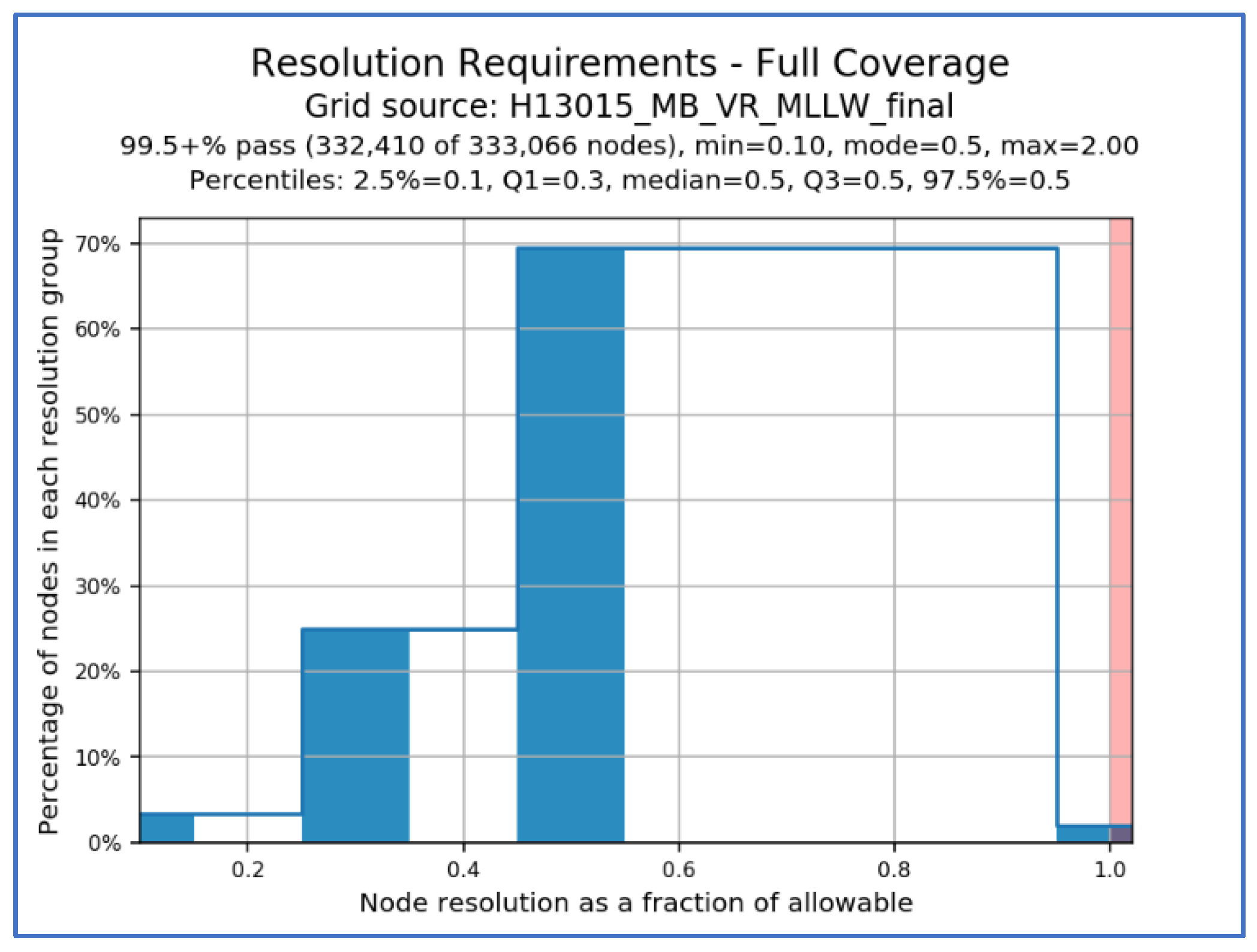
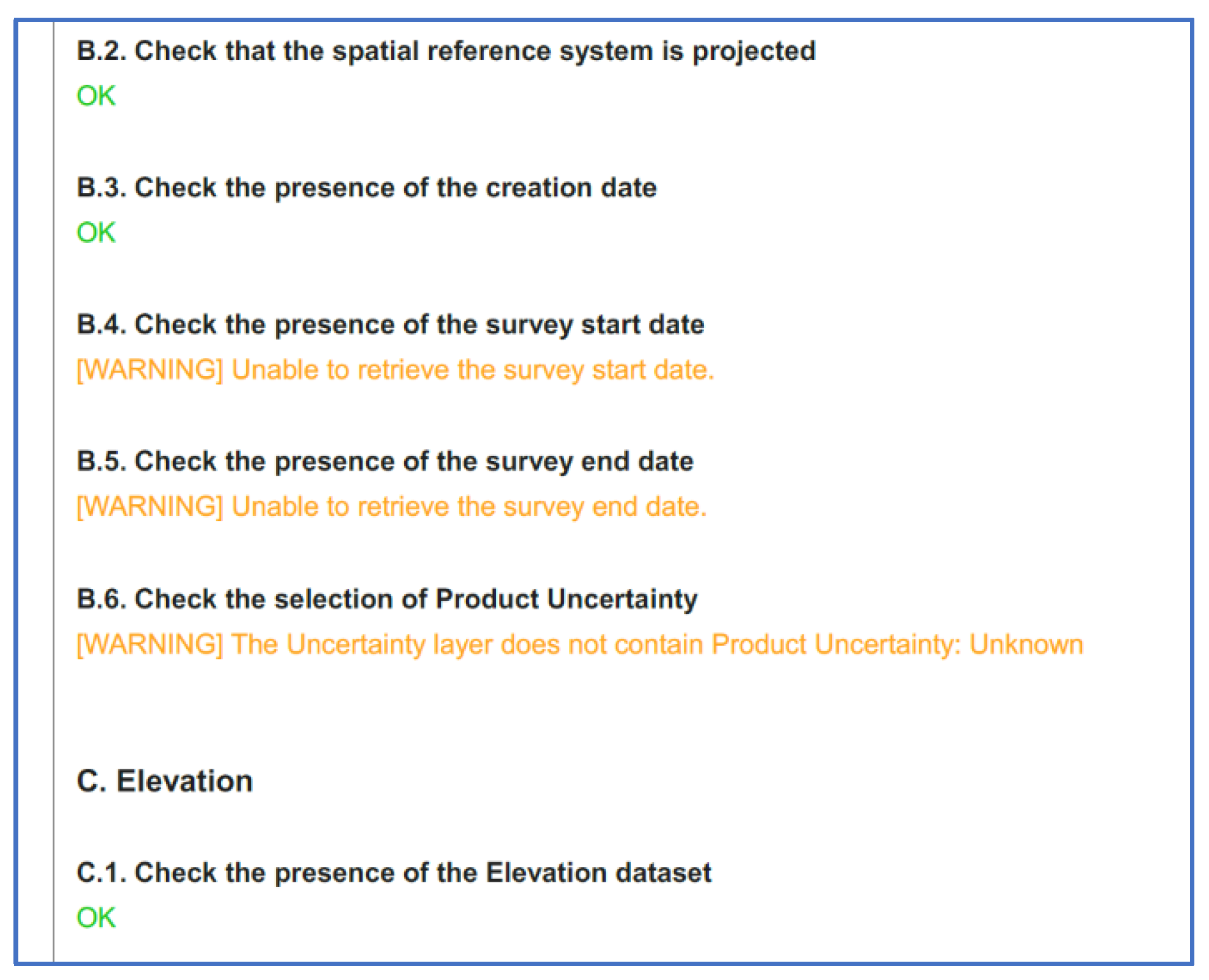
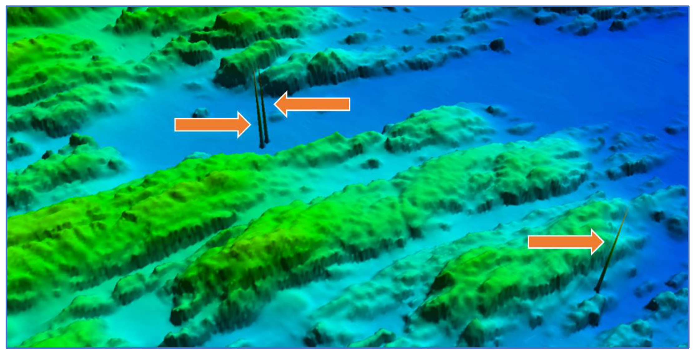
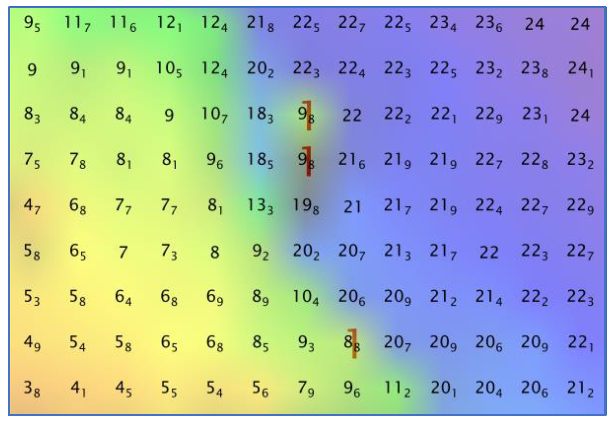
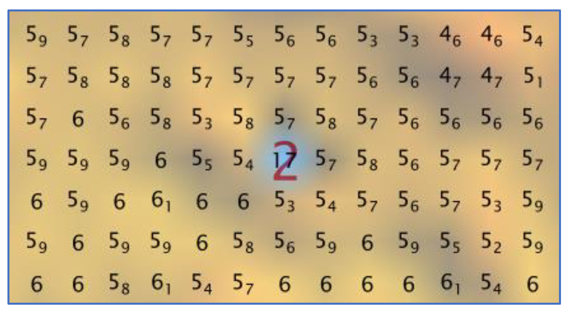
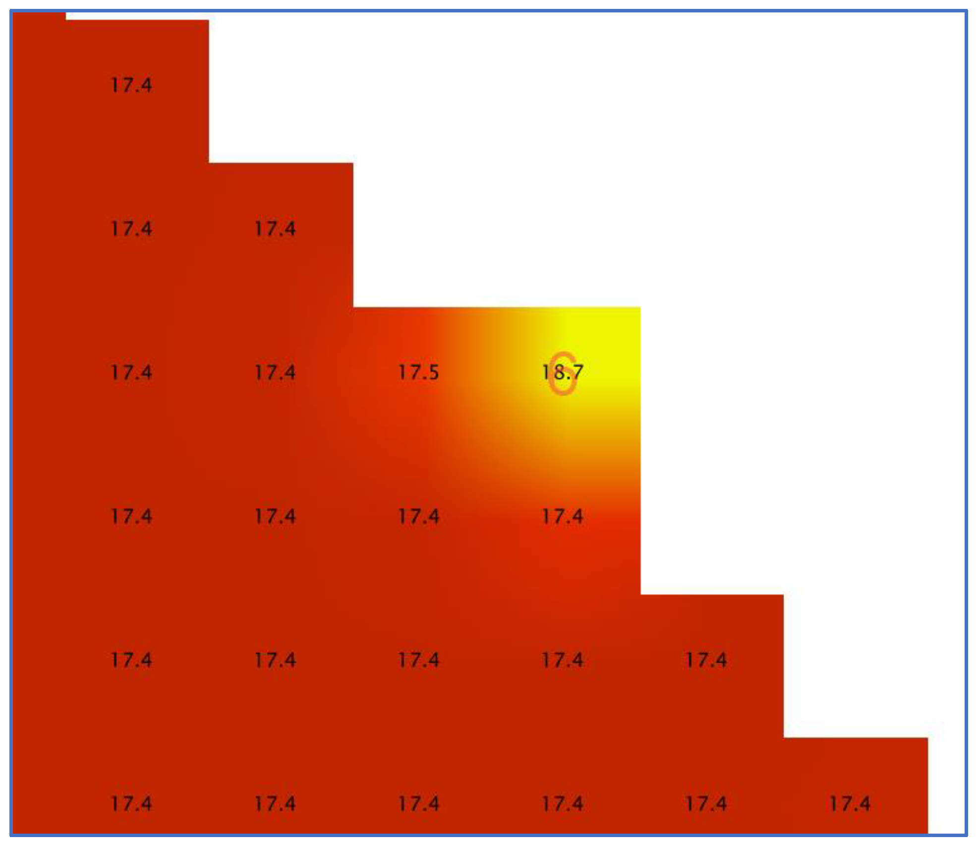
2.1. Grid Quality Control

The fliers are often associated with suboptimal data filtering and cleaning, both automatic and manual, of high-density hydrographic surveys such as the ones acquired with multibeam echosounders [1,5,22,23]. A hydrographic data reviewer may identify the presence of such fliers using traditional methods, such as inspection using 2D/3D viewers or evaluation of specific grid metrics, and/or shoal-biased sounding selection [24,25]. However, these methods are inherently error-prone and quite subjective, with the result that several fliers can be easily missed during the hydrographic data review [14]. As such, it is not surprising that in 2015, the NOAA Hydrographic Surveys Division reported that nearly 25% of the surveys received were affected by fliers [26]. Even adopting more than one of the methods mentioned, it is challenging to identify all the fliers that may be present on a grid with several millions of cells [16]. Scanning the grid with automated algorithms that flag potential anomalies not only supports the job of the reviewer, but also builds confidence in the performed manual evaluation. This is especially true in areas with rough seafloor morphology, where small fliers can be easily confused with natural features (Figure 1) [27].

A manual grid inspection for identification of all the holidays is a comparable challenge [26]. However, while there are different types of fliers (e.g., isolated vs. clustered), the definition of what is considered a significant holiday is quite objective and is usually outlined in the survey requirements [13]. There is great advantage in developing a robust algorithmic translation to automatically scan for potential holidays.

Several hydrographic specifications—for instance, the NOAA Hydrographic Survey Specifications and Deliverables (HSSD) [13]—allow for the manual selection of specific soundings (designated soundings) being judged as particularly significant and thus, requiring their depth value to be enforced in the grid. When designated soundings are in use, their automated review is beneficial to evaluate their alignment with the specifications (for instance, to identify the misuse of designated soundings). The alternative to such automated review is tedious, manual work based on vertical or horizontal measurements in the surroundings of each designated sounding.

It is also quite common that the survey specifications have requirements for the grid’s specific statistical metrics (e.g., uncertainty, density of soundings) [28]. Although software providers usually support calculation of statistical grid layers, it is not common for the validation against hydrographic specifications to be included. The translation of such rules into an automated procedure—returning a pass or fail indication and/or providing a visual representation of the rules—has the positive effects of simplifying the job of the reviewer, enforcing consistent interpretation across all the datasets, and making any future customization much easier.

Ensuring that the created products fulfill format specifications (e.g., the BAG Format Specification Document [18]) is also of great value. Such a fulfillment eases the data interoperability, ensuring that internal and public users of a survey bathymetric grid can properly access and interpret the collected survey data.

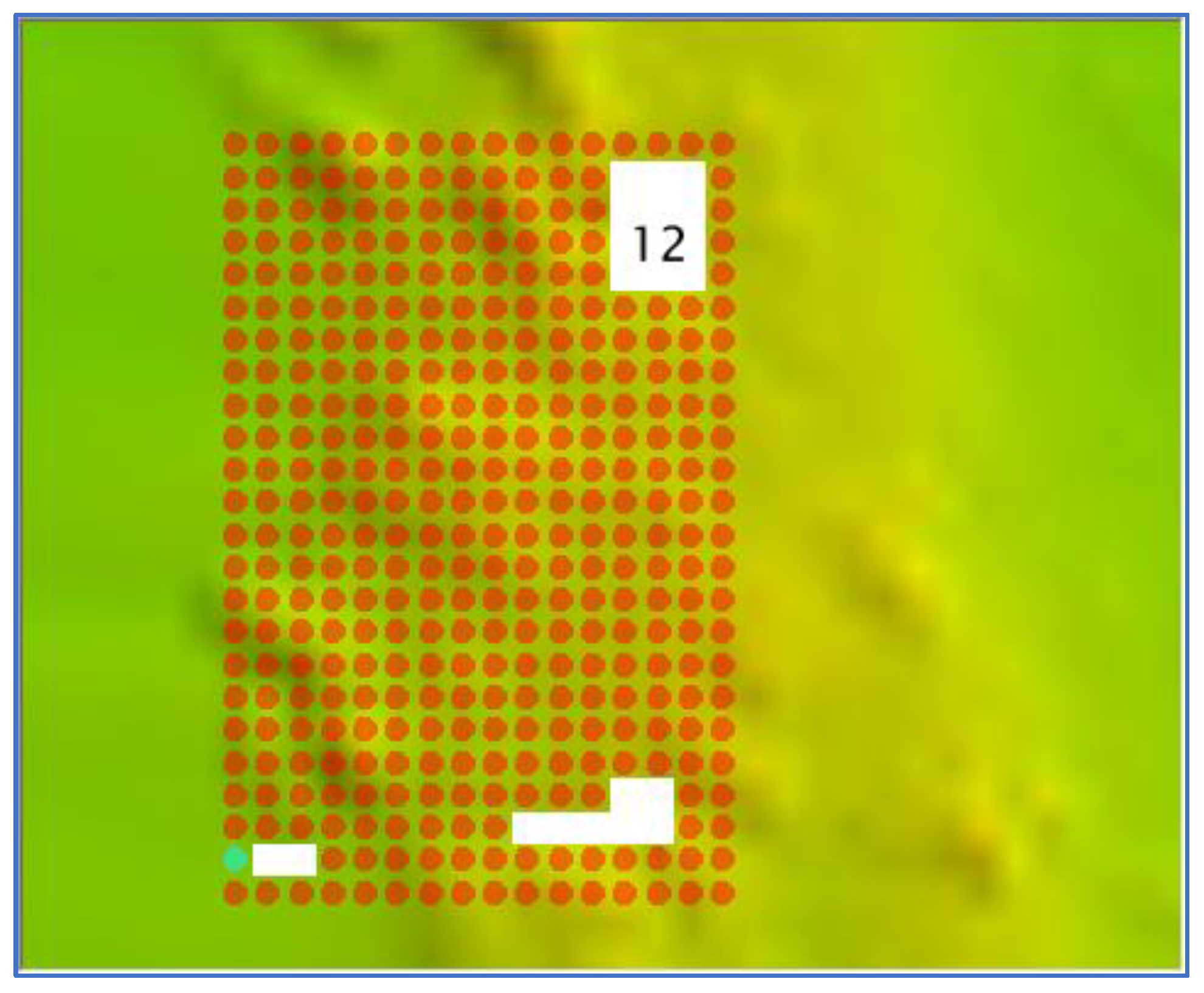
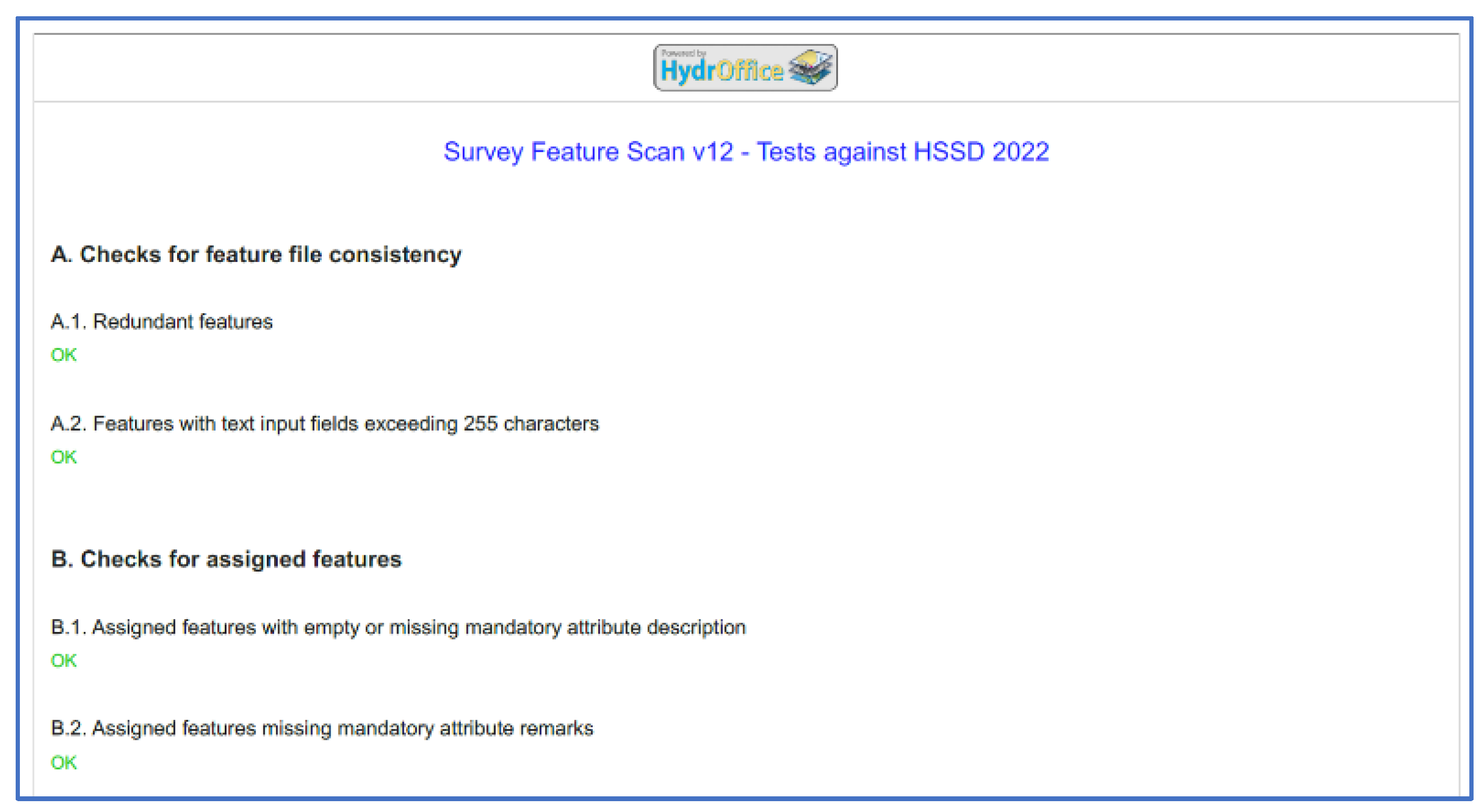
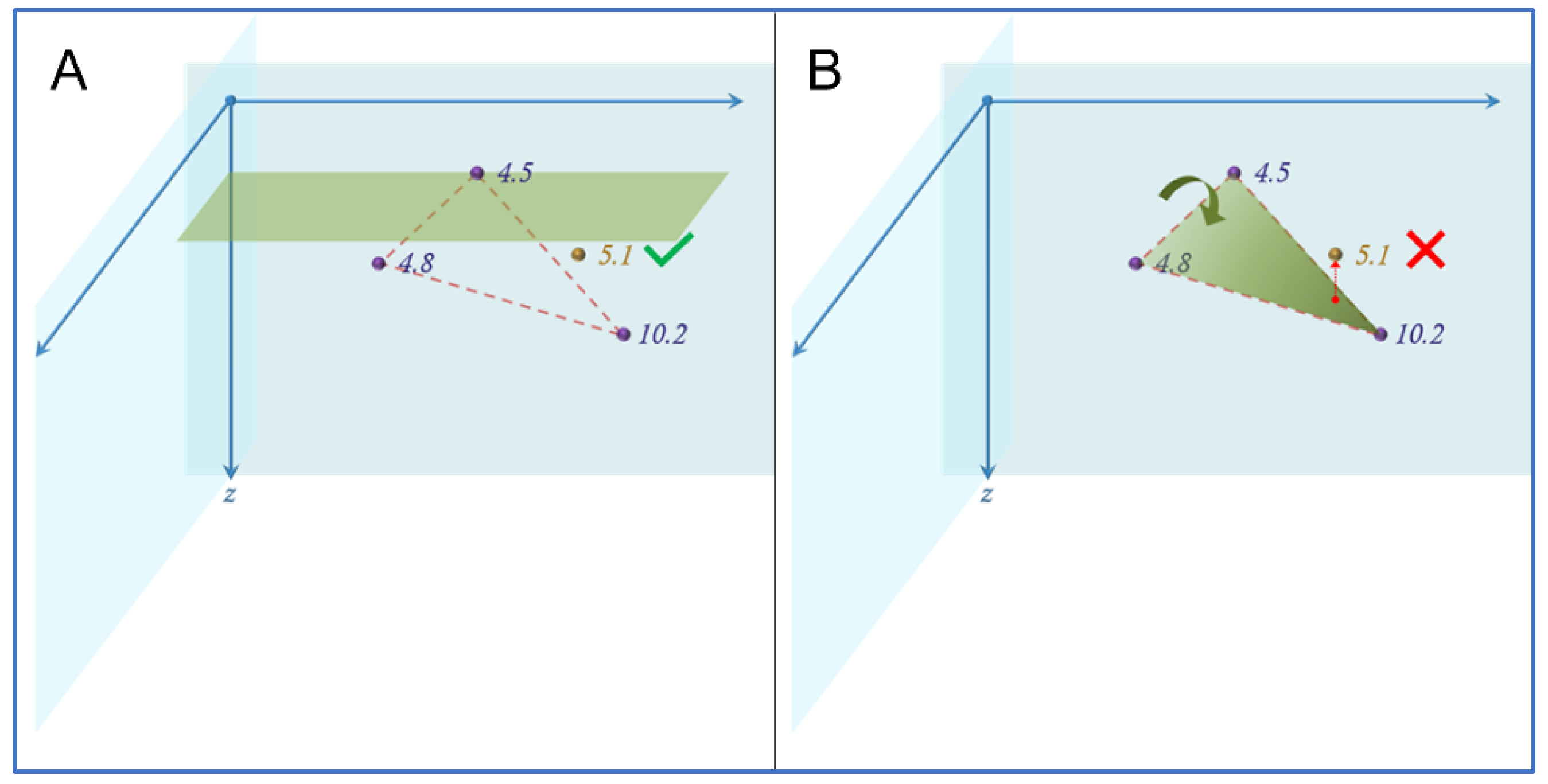
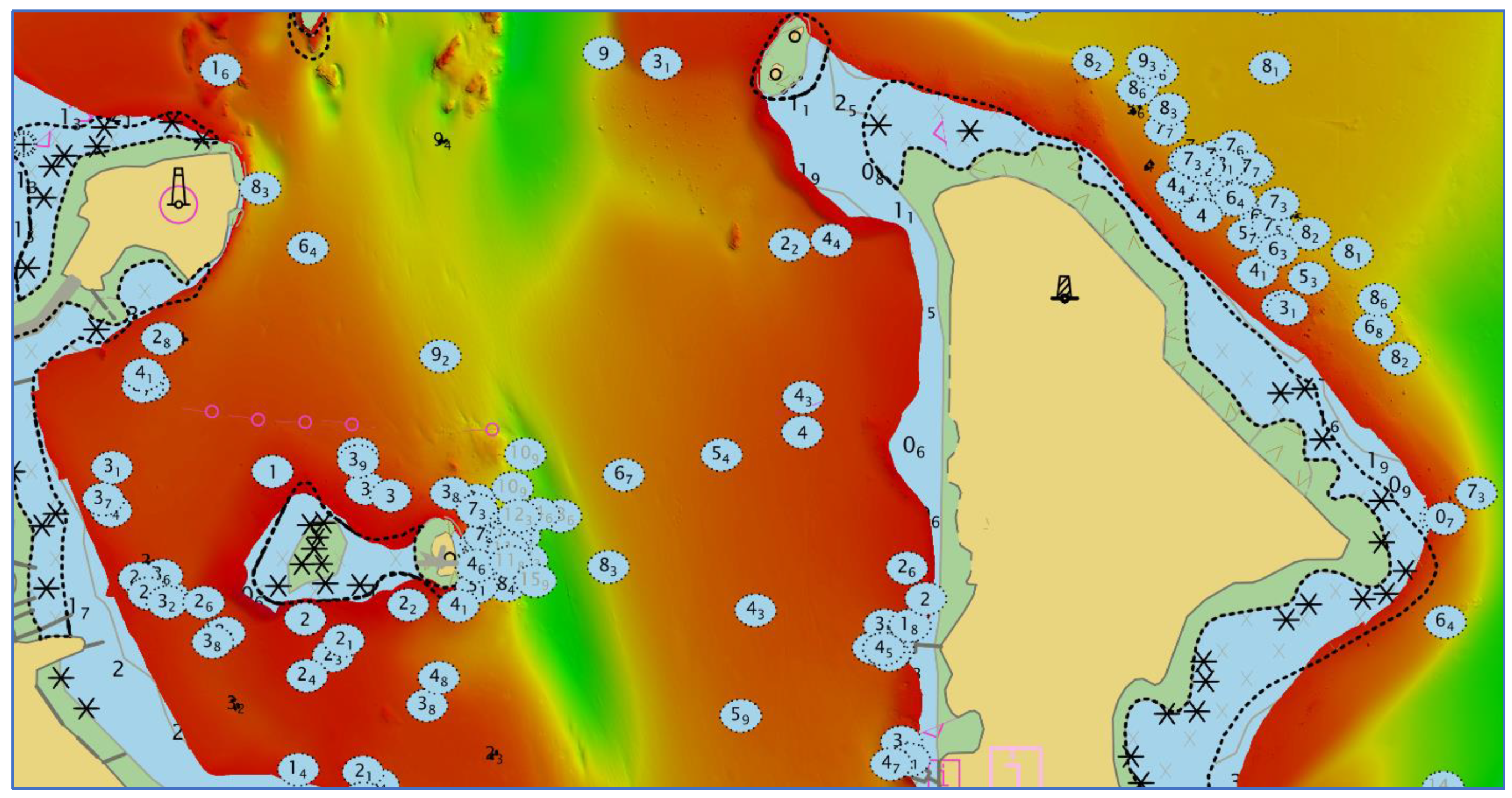
2.2. Significant Features Validation

The outcome of a hydrographic survey is not usually limited to a bathymetric point cloud and the bathymetric grid derived from it. The surveyor is quite often called to integrate the collected bathymetry with a set of significant features. These features may carry a variety of information that may interest the seafarers, such as dangers, or auxiliary aids to navigation. Although several manufacturer-specific methods for feature validation exist, it is beneficial for a hydrographic office to be able to not only enforce specific feature validation tests, but also to run them independently of the specific processing software in use.

In approach and harbor areas, the number of significant features can be large and the review of the associated metadata time consuming, error-prone, and particularly tedious (Figure 2). In addition, the task at hand is made even more challenging by the necessity of adhering to all the rules required to ensure proper cartographic attribution. However, most of the mentioned requirements do not require judgement by a skilled analyst and thus, are easy to automate. Furthermore, redundant features and attributes can also be easily identified and reported to the hydrographic data reviewer.

Finally, significant features with an associated depth can be evaluated against the bathymetric grid to ensure that the grid and the feature attributes are consistent [13]. This latter task may appear simple, but the required amount of time quickly increases in nearshore areas saturated with features [17].

2.3. Survey Soundings and Chart Adequacy

High-density hydrographic surveys commonly consist of millions of survey soundings [1,7]. A bathymetric grid may be seen as a spatial filter for those hydrographic datasets to reduce the number of soundings based on reliable criteria. To preserve the safety of navigation, a common requirement is to assign the shoalest depth value among all the soundings within each grid cell [29]. However, gridding is just one of the possible methods used to identify a meaningful subset of the survey dataset to be used for cartographic processes [30,31,32].

During the hydrographic data review, it is often necessary to compare two different sets of depth values, e.g., a sounding selection. A common requirement is to compare a dense selection from the hydrographic survey under review with a sparser set of soundings and depth-attributed features derived from the chart. From such a comparison, shoals and dangers to navigation can be easily identified [15]. A similar procedure can be used to validate a set of newly proposed charted soundings against the original dense survey dataset. In both cases, the denser of the two sets may normally consist of tens of thousands of soundings, thus the manual execution of a similar task by the reviewer may end with several inconsistencies, some of them potentially associated with high safety-of-navigation risks [15]. As such, the development of automated procedures targeting the comparison of sets of depths has been critical for supporting the review process and specifically, to ensure that no critical shoal depths were missed.

3. Implementation and Results

In the past few years, the automated procedures outlined in the previous section have been implemented in two software applications, called QC Tools and CA Tools, developed in the HydrOffice framework [15,16]. HydrOffice (www.hydroffice.org, accessed on 8 August 2022) is an open-source collaborative project to develop a research software environment containing applications to strengthen all phases of the ping-to-public process in order to facilitate data acquisition, automate and enhance data processing, and improve hydrographic products [6].

QC Tools and CA Tools are currently implementing the survey specifications (i.e., the NOAA HSSD [13]) and other internal best practices of the NOAA Office of Coast Survey. Both tools are publicly available in Pydro—a free and open Python distribution—and as stand-alone applications (downloadable from the HydrOffice website: https://www.hydroffice.org/qctools/main, accessed on 8 August 2022; and https://www.hydroffice.org/catools/main, accessed on 8 August 2022) [33]. The stand-alone applications are currently distributed only for Microsoft Windows, although the underlying source code is cross-platform (e.g., Linux).

The algorithmic interpretation of the Office of Coast Survey’s directives in both tools is regularly updated to reflect relevant changes introduced by the agency. The tools are also useful to train new personnel by helping them identify grid inconsistencies and feature issues, as well as in the interpretation of the survey specifications.

The code base of both software tools is similarly organized, consisting of a library, where the algorithms are implemented, and mechanisms to access such a library:

• Several scripts that can be used as a foundation to create new, custom algorithms.
• A command line interface useful to integrate some of the algorithms in the processing pipeline.
• An application with a graphical user interface (the app).

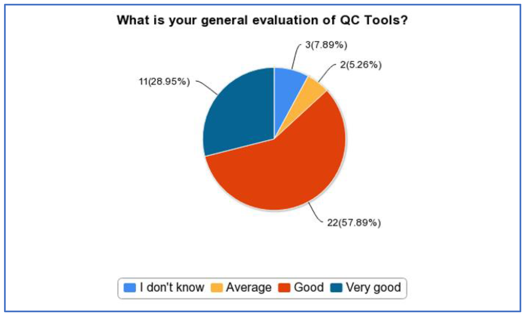
Both apps have a similar design to ease the user experience: they are arranged with a few main tabs and several sub-tabs. Specifically, the QC Tools app is organized into three main tabs. The first two are the Survey Validation tab and the Chart Review tab; these provide access to the QC tools themselves. The CA Tools app is organized into two main tabs, with the first one being the Chart Adequacy tab, providing access to the chart adequacy tools. Finally, for both apps, the last tab (the Info tab) includes support material, such as access to offline/online documentation and license information.

3.1. QC Tools

QC Tools provides automated procedures to:

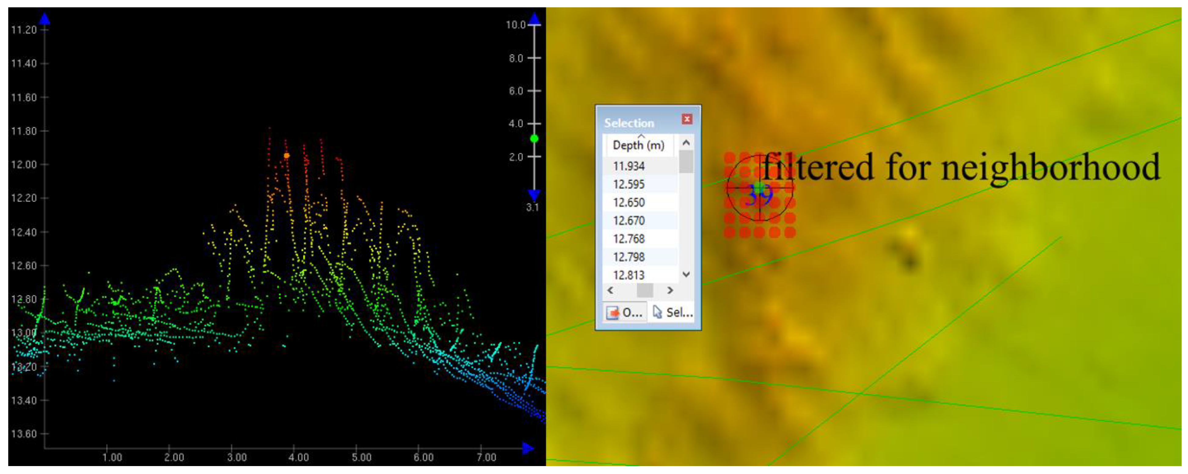
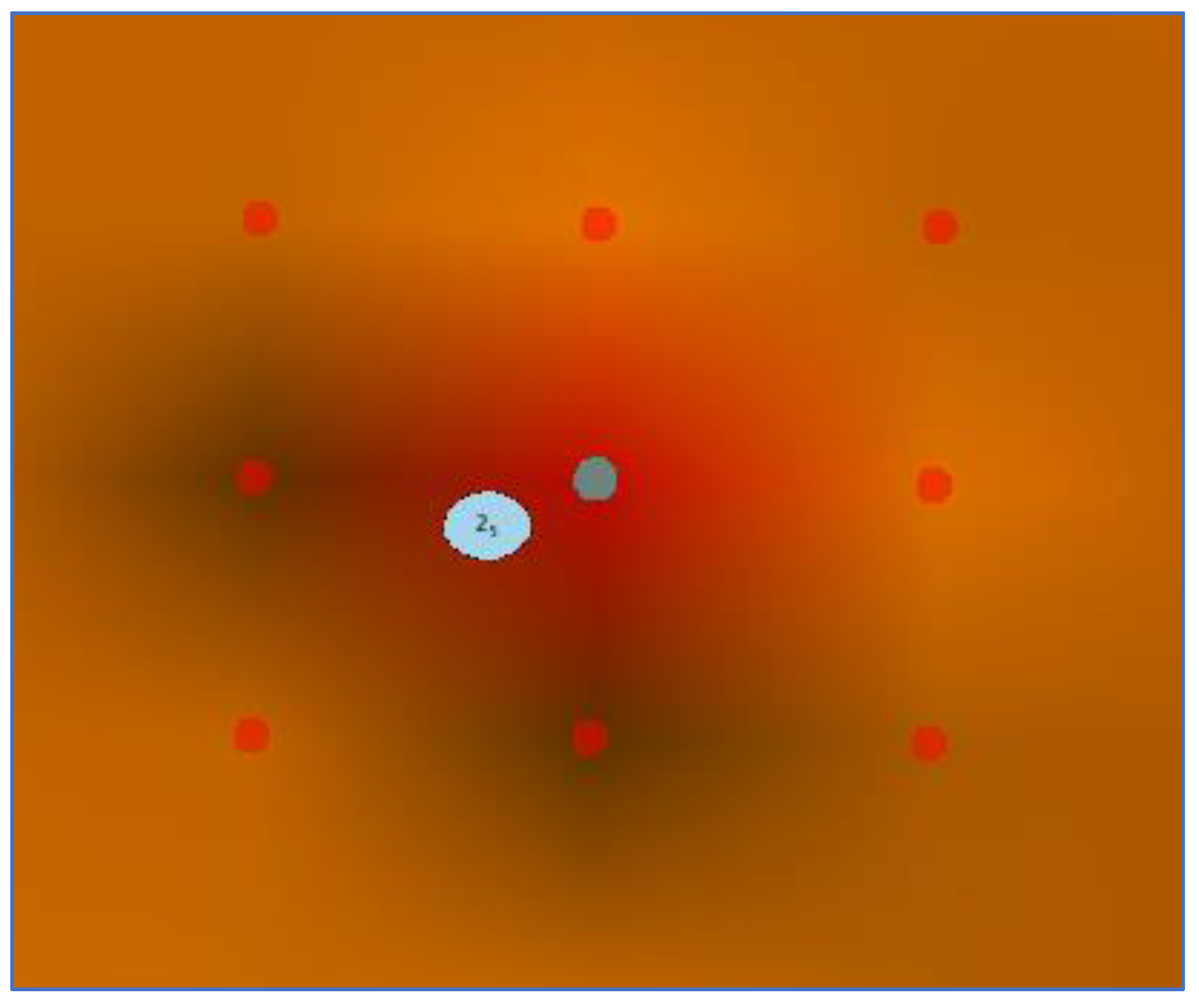
• Detect candidate fliers and significant holidays in gridded bathymetry.
• Ensure that gridded bathymetry fulfills statistical requirements (e.g., sounding density and uncertainty).
• Check the validity of BAG files containing gridded bathymetry.
• Scan selected designated soundings to ensure their significance.
• Validate the attributes of significant features.
• Ensure consistency between grids and significant features.
• Extract seabed area characteristics for public distribution.
• Analyze the folder structure of a survey dataset for proper archival.

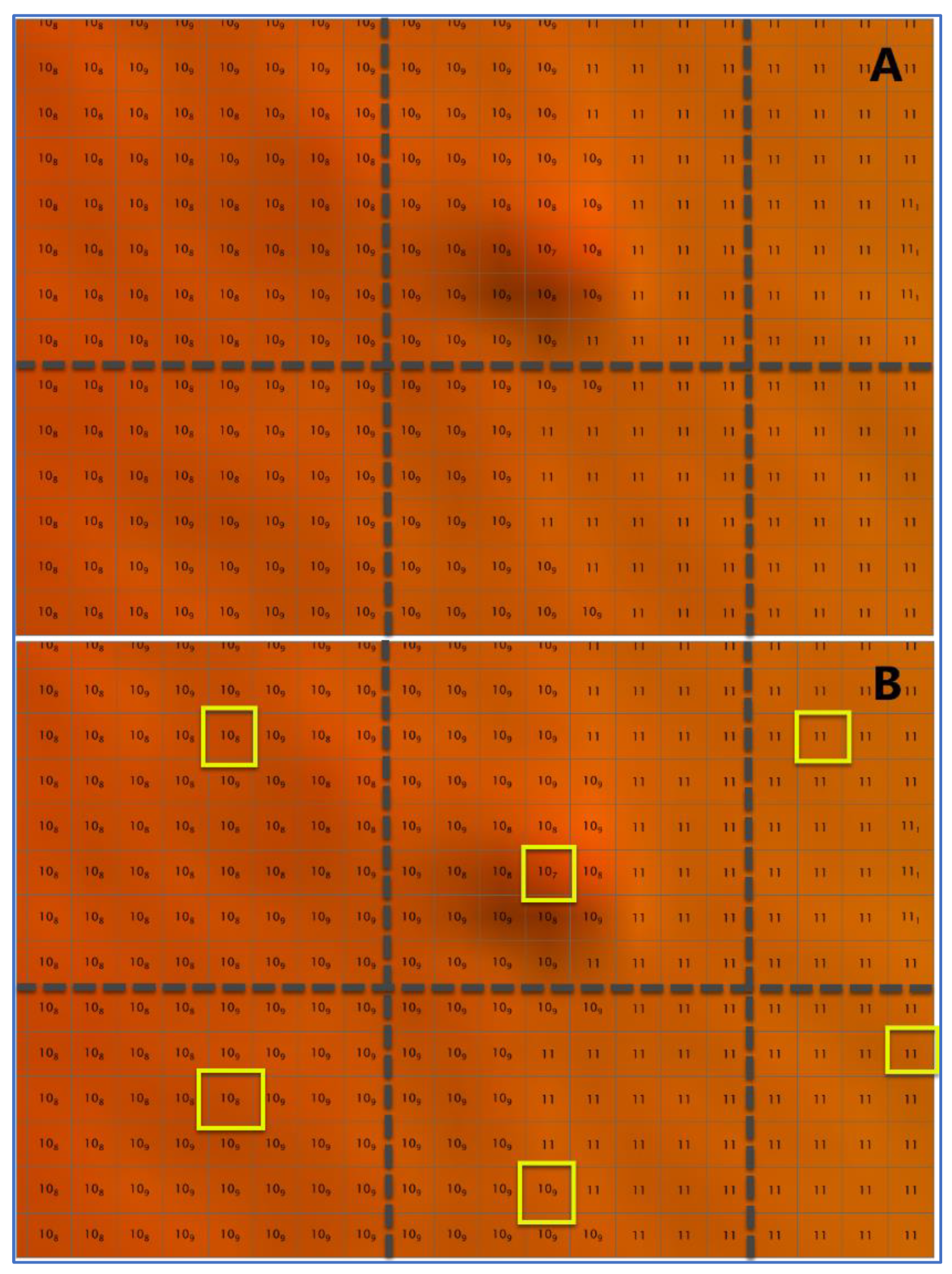
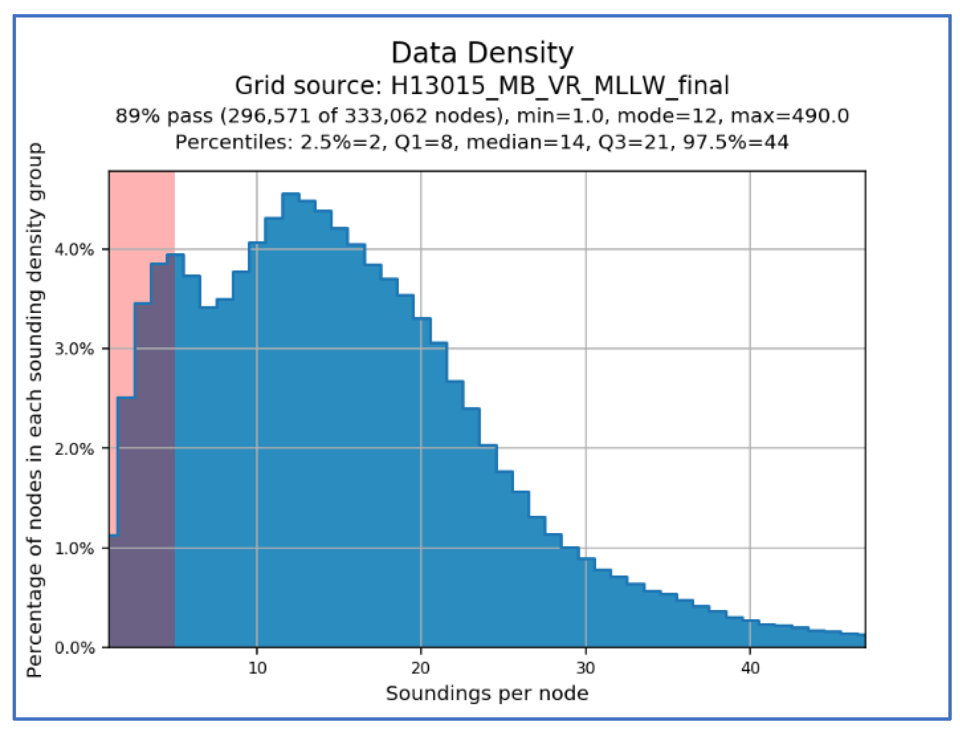
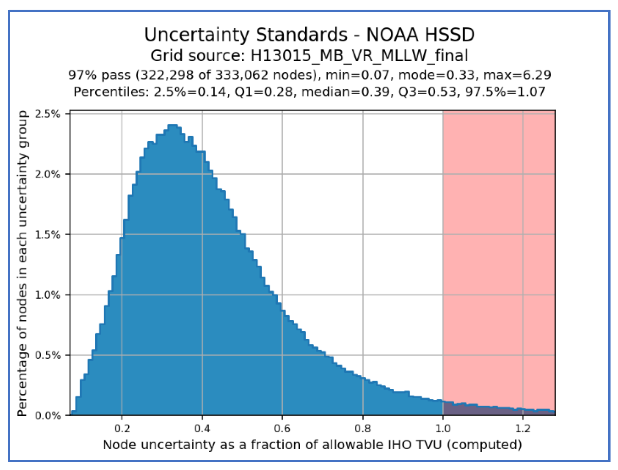
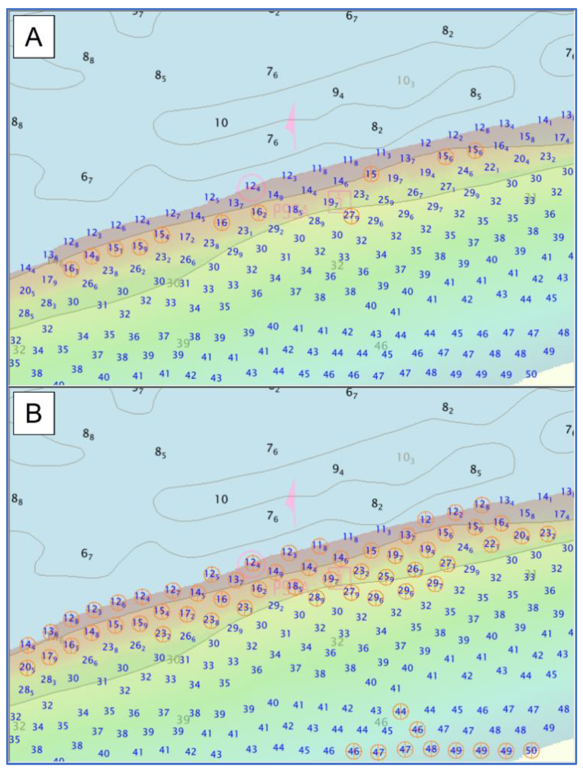
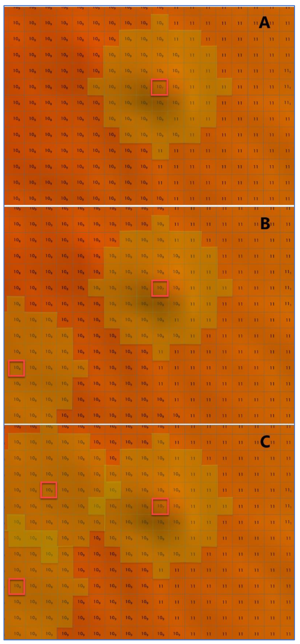
3.1.1. Grid Quality Controls

The Detect Fliers tool, also known as Flier Finder, aims to identify potential fliers in dense bathymetric grids. As previously mentioned, fliers can come in different types. As such, seven distinct algorithms have been developed over the past several years (see

Table 1. Algorithms currently in use by the Detect Fliers tool.

Detect Fliers’ Algorithm	Search Height Required
Laplacian Operator	Yes
Gaussian Curvature	No
Adjacent Cells	Yes
Edge Slivers	Yes
Isolated Nodes	No
Noisy Edges	No
Noisy Margins	No

). Some of the algorithms require a search height as a parameter. When required by the algorithm, the search height may be used to tune the sensitivity to potential anomalies. For instance, the optimal search height on a relatively flat seafloor and shallow waters is usually smaller than for a dynamic area covered by a deep-water survey. Although the search height may be manually defined by the reviewer, the suggested solution is to have it automatically derived by an internal algorithm implementing a heuristic approach function of the median depth, depth variability, and grid roughness. The automated estimation of the search height helps standardize the hydrographic data review.

The Laplacian Operator (Figure 3), the Gaussian Curvature (Figure 4), and the Adjacent Cells algorithms aim to detect shoal or deep spikes throughout the entirety of the bathymetric grid, whereas the Edge Slivers algorithm identifies potential fliers—mainly due to sparse data—on grid edges. The Isolated Node algorithm detects the presence of soundings detached from the main bathymetric grid that are often difficult to identify manually. Both the Noisy Edges (Figure 5) and Noisy Margins algorithms are tailored to identify fliers along noisy swath edges using the International Hydrographic Organization’s S-44′s Total Vertical Uncertainty (in place of the mentioned search height) [34]. The development of these latter algorithms was triggered by the fact that depth values associated with isolated nodes or on the grid edges are often unreliable when derived from the outmost beams of a bathymetric swath [35,36].

The Detect Holidays tool, also known as Holiday Finder, performs a grid search for holidays. The algorithm first identifies all the grid holidays, regardless of their size; then those holidays are tested against the survey specifications. Following the NOAA HSSD, the tool assess holidays based on the required survey coverage: either Full Coverage (Figure 6) or Object Detection (the latter having more restrictive criteria) [13]. The algorithm has been coded to calculate the holiday size (in number of nodes) based on the minimum allowable resolution and the grid resolution, but it is flexible for adjustments to different holiday descriptions.

The Grid QA tool performs statistical analysis on the bathymetric grid, looking at metrics such as data density (Figure 7), uncertainty (Figure 8), and, for variable-resolution grids, resolution requirements (Figure 9). Similar to the Detect Holidays tool, the current requirements are based on the NOAA HSSD [13], but can be adjusted to meet other specifications.

The BAG Checks tool ensures compliance with the Open Navigation Surface Bathymetry Attributed Grid (BAG) format [18] for gridded bathymetry and, if selected, for additional NOAA-specific requirements. The algorithm checks the overall structure of the file, the metadata content, the elevation layer, the uncertainty layer, and the tracking list (an example of output is provided in Figure 10). It also performs a compatibility check with the popular GDAL software library and tools [37].

The Scan Designated tool validates the soundings designated by the surveyor against the bathymetric grid to ensure their significance (according to NOAA HSSD specifications) [13]. Discrepancies are automatically highlighted for the reviewer (see Figure 11).

3.1.2. Significant Features Validation

The Scan Features tool checks the required S-57 attribution (e.g., [13]) for features that will be passed through the charting pipeline after the hydrographic data review (an example output report is shown in Figure 12). The tool provides several options to tailor the result to specific needs. For example, it is possible to switch between a field profile and an office profile based on the stage of the review pipeline at which the tool is executed. Other useful options are the version of the specification to be applied and additional checks, such as the image file naming convention, or the format of specific attributes (e.g., the date and the identification of the survey).

The Check VALSOU tool evaluates all features against the corresponding grid nodes to ensure that the value of the sounding (VALSOU) and position matches what is present in the bathymetric grid. This tool not only ensures parity between feature depth and the grid, but it will also ensure that the depth entered is the most shoal depth among the nine grid nodes of the feature (see Figure 13).

3.2. CA Tools

CA Tools provides automated procedures to:

• Identify chart discrepancies for a bathymetric grid or a set of survey soundings.
• Select a significant set of soundings from a bathymetric grid.

The first step of the Chart Adequacy algorithm is to build a triangulated irregular network (TIN) from existing chart soundings and features; then it matches the dense set of survey soundings within the triangles of the TIN. At this point, the algorithm may apply two different testing methods: the Shoalest Depth method and the Tilted Triangle method. The Shoalest Depth testing method implements a longstanding Office of Coast Survey’s best practice (called Triangle Rule) for the comparison of sounding sets (see Figure 14, pane A). In practice, any survey sounding shoaler than any of the three vertices of its containing triangle is marked as a potential problem. To overcome the inherent limitations of the Triangle Rule, the tilted-triangle test described in [6] (Figure 14, pane B) has been made available as the Triangle Rule testing method (see Figure 15). Due to the complexity of nautical charts, the algorithm also enforces additional sounding-in specific-feature tests [6]. The algorithm also computes the magnitude of the discrepancy against the chart and adds it as an S-57 attribute, allowing the identified soundings to be sorted. In this manner, the most significant discrepancies (and potential dangers to navigation) are identified immediately.

To summarize, the Chart Adequacy tool implements a method of sounding comparison that has two distinct applications: hydrographic survey review (as a quick identification of dangers to navigation) and chart review (as a method of validating a prospective chart sounding selection prior to its application).

The Sounding Selection tool creates a sounding selection from a bathymetric grid. Once created, the sounding selection can also be used to compare the survey data to the chart using the described Chart Adequacy tool. In fact, the initial motivation to create such a tool was to provide a mechanism to evaluate chart adequacy directly from a bathymetric grid. Two sounding selection algorithms are currently available: Moving Window and Point Additive. The Moving Windows algorithm is quite simple: the bathymetric grid is divided in square areas based on the size of a user-defined search radius (Figure 16, pane A); then the shallowest depth is selected within each area (Figure 16, pane B). The Point Additive algorithm iteratively selects the shallowest point in a bathymetric grid and then removes all cells within the radius of the selected sounding (Figure 17). The iteration continues until there are no remaining data points.

4. Discussion

Applied to a large number of hydrographic surveys in recent years, the automated procedures in HydrOffice QC Tools and CA Tools have been shown to improve both the quality and timeliness of the review process [6,26]. An increased confidence in the final data produced was also observed, especially among personnel in training [6]. As such, the combined effect of applying these procedures is a novel holistic approach to hydrographic data review.

Both tools focus on several challenges present in the ping-to-public workflow, adopting a divide et impera (divide and conquer) approach and tackling the most time critical and error-prone steps [6]. By design, these tools are intended to be complementary to an existing hydrographic processing pipeline, providing valuable, and sometimes critical, supplementation of operator assessment with automated scanning over large datasets.

Although tailored to NOAA’s processing and validation chain, the automated procedures are generically applicable to other hydrographic offices. The modular structure, inherited from the HydrOffice architecture, allows for the customization of the algorithms to different survey specifications. Furthermore, given that the code is neatly separated from the graphical user interface, the creation of stand-alone scripts is simple, both for local and cloud-based execution. For similar reasons, the code implementation of the specifications can be easily updated as the directives evolve.

These tools provide solutions for cases where software manufacturers are unable, or unwilling, to support the level of customization required by the hydrographic office. At the same time, these tools unambiguously provide algorithmic interpretation and evaluation of survey specifications. With a strong foundation of version-controlled algorithms, these tools represent a solid base for expanding automation in the future.

The feedback from the users within NOAA is positive, with the project receiving enthusiastic reviews from users, in terms of both frequency of use (Figure 18) and general evaluation (Figure 19) [6]. Furthermore, recently observed improvements in the Office of Coast Survey’s data quality and timeliness has been partially attributed to the field implementation of these tools [3]. Given the similarities of review procedures among hydrographic offices, the described approach has generated interest in the ocean mapping community. This is mainly because the extent of the algorithmic interpretation of agency specifications represents the foundation for the adoption of automated workflows [16].

A known limitation shared across the current implementations of both QC Tools and CA Tools is that visualizing their output requires an external GIS application that supports open hydrographic formats, such as BAG and S-57. Although most hydrographic software packages can read these formats, there are intrinsic limitations regarding how data reviewers can interact with the output. A possible solution to such an issue may be the creation of a plugin to interface the algorithm with an open GIS software, such as QGIS [38]. Such a solution will be explored as part of future development efforts.

References

1. Le Deunf, J.; Debese, N.; Schmitt, T.; Billot, R. A Review of Data Cleaning Approaches in a Hydrographic Framework with a Focus on Bathymetric Multibeam Echosounder Datasets. Geosciences 2020, 10, 254. [Google Scholar] [CrossRef]
2. Wlodarczyk-Sielicka, M.; Blaszczak-Bak, W. Processing of Bathymetric Data: The Fusion of New Reduction Methods for Spatial Big Data. Sensors 2020, 20, 6207. [Google Scholar] [CrossRef] [PubMed]
3. Evans, B. What are our Shared Challenges. In Proceedings of the NOAA Field Procedures Workshop, Virginia Beach, VA, USA, 24–26 January 2017. [Google Scholar]
4. Calder, B. Multi-algorithm swath consistency detection for multibeam echosounder data. Int. Hydrogr. Rev. 2007, 8. Available online: https://journals.lib.unb.ca/index.php/ihr/article/view/20778 (accessed on 8 August 2022).
5. Deunf, J.L.; Khannoussi, A.; Lecornu, L.; Meyer, P.; Puentes, J. Automatic Data Quality Assessment of Hydrographic Surveys Taking Into Account Experts’ Preferences. In Proceedings of the OCEANS 2021: San Diego–Porto, Porto, Portugal, 20–23 September 2021; pp. 1–10. [Google Scholar] [CrossRef]
6. Masetti, G.; Faulkes, T.; Kastrisios, C. Hydrographic Survey Validation and Chart Adequacy Assessment Using Automated Solutions. In Proceedings of the US Hydro 2019, Biloxi, MS, USA, 19–21 March 2019. [Google Scholar] [CrossRef]
7. Hughes Clarke, J.E.; Mayer, L.A.; Wells, D.E. Shallow-water imaging multibeam sonars: A new tool for investigating seafloor processes in the coastal zone and on the continental shelf. Mar. Geophys. Res. 1996, 18, 607–629. [Google Scholar] [CrossRef]
8. Ladner, R.W.; Elmore, P.; Perkins, A.L.; Bourgeois, B.; Avera, W. Automated cleaning and uncertainty attribution of archival bathymetry based on a priori knowledge. Mar. Geophys. Res. 2017, 38, 291–301. [Google Scholar] [CrossRef]
9. Eeg, J. On the identification of spikes in soundings. Int. Hydrogr. Rev. 1995, 72, 33–41. [Google Scholar]
10. Debese, N.; Bisquay, H. Automatic detection of punctual errors in multibeam data using a robust estimator. Int. Hydrogr. Rev. 1999, 76, 49–63. [Google Scholar]
11. Hughes Clarke, J.E. The Impact of Acoustic Imaging Geometry on the Fidelity of Seabed Bathymetric Models. Geosciences 2018, 8, 109. [Google Scholar] [CrossRef]
12. Bottelier, P.; Briese, C.; Hennis, N.; Lindenbergh, R.; Pfeifer, N. Distinguishing features from outliers in automatic Kriging-based filtering of MBES data: A comparative study. In Geostatistics for Environmental Applications; Springer: Berlin/Heidelberg, Germany, 2005; pp. 403–414. [Google Scholar] [CrossRef]
13. NOAA. Hydrographic Surveys Specifications and Deliverables; National Oceanic and Atmospheric Administration, National Ocean Service: Silver Spring, MD, USA, 2022. [Google Scholar]
14. Jakobsson, M.; Calder, B.; Mayer, L. On the effect of random errors in gridded bathymetric compilations. J. Geophys. Res. Solid Earth 2002, 107, ETG 14-1–ETG 14-11. [Google Scholar] [CrossRef]
15. Masetti, G.; Faulkes, T.; Kastrisios, C. Automated Identification of Discrepancies between Nautical Charts and Survey Soundings. ISPRS Int. J. Geo-Inf. 2018, 7, 392. [Google Scholar] [CrossRef] [Green Version]
16. Wilson, M.; Masetti, G.; Calder, B.R. Automated Tools to Improve the Ping-to-Chart Workflow. Int. Hydrogr. Rev. 2017, 17, 21–30. [Google Scholar]
17. IHO. S-57: Transfer Standard for Digital Hydrographic Data; International Hydrographic Organization: Monte Carlo, Monaco, 2000. [Google Scholar]
18. Calder, B.; Byrne, S.; Lamey, B.; Brennan, R.T.; Case, J.D.; Fabre, D.; Gallagher, B.; Ladner, R.W.; Moggert, F.; Paton, M. The open navigation surface project. Int. Hydrogr. Rev. 2005, 6, 9–18. [Google Scholar]
19. Quick, L.; Foster, B.; Hart, K. CARIS: Managing bathymetric metadata from “Ping” to Chart. In Proceedings of the OCEANS 2009, Biloxi, MS, USA, 26–29 October 2009; pp. 1–9. [Google Scholar] [CrossRef]
20. Younkin, E. Kluster: Distributed Multibeam Processing System in the Pangeo Ecosystem. In Proceedings of the OCEANS 2021: San Diego–Porto, Porto, Portugal, 20–23 September 2021; pp. 1–6. [Google Scholar] [CrossRef]
21. van Rossum, G. The Python Language Reference: Release 3.6.4; 12th Media Services: Suwanee, GA, USA, 2018; p. 168. [Google Scholar]
22. Calder, B.; Mayer, L. Robust Automatic Multi-beam Bathymetric Processing. In Proceedings of the US Hydro 2001, Norfolk, VA, USA, 22–24 May 2001. [Google Scholar]
23. Hou, T.; Huff, L.C.; Mayer, L.A. Automatic detection of outliers in multibeam echo sounding data. In Proceedings of the US Hydro 2001, Norfolk, VA, USA, 22–24 May 2001. [Google Scholar]
24. Mayer, L.A. Frontiers in Seafloor Mapping and Visualization. Mar. Geophys. Res. 2006, 27, 7–17. [Google Scholar] [CrossRef]
25. Mayer, L.A.; Paton, M.; Gee, L.; Gardner, S.V.; Ware, C. Interactive 3-D visualization: A tool for seafloor navigation, exploration and engineering. In Proceedings of the OCEANS 2000 MTS/IEEE Conference and Exhibition, Conference Proceedings (Cat. No.00CH37158). Providence, RI, USA, 11–14 September 2000; Volume 912, pp. 913–919. [Google Scholar] [CrossRef]
26. Gonsalves, M. Survey Wellness. In Proceedings of the NOAA Coast Survey Field Procedures Workshop, Virginia Beach, VA, USA, 27–20 January 2015. [Google Scholar]
27. Briggs, K.B.; Lyons, A.P.; Pouliquen, E.; Mayer, L.A.; Richardson, M.D. Seafloor Roughness, Sediment Grain Size, and Temporal Stability; Naval Research Lab: Washington, DC, USA, 2005. [Google Scholar]
28. Hare, R.; Eakins, B.; Amante, C. Modelling bathymetric uncertainty. Int. Hydrogr. Rev. 2011, 9, 31–42. [Google Scholar]
29. Armstrong, A.A.; Huff, L.C.; Glang, G.F. New technology for shallow water hydrographic surveys. Int. Hydrogr. Rev. 1998, 2, 27–41. [Google Scholar]
30. Dyer, N.; Kastrisios, C.; De Floriani, L. Label-based generalization of bathymetry data for hydrographic sounding selection. Cartogr. Geogr. Inf. Sci. 2022, 49, 338–353. [Google Scholar] [CrossRef]
31. Zoraster, S.; Bayer, S. Automated cartographic sounding selection. Int. Hydrogr. Rev. 1992, 1, 103–116. [Google Scholar]
32. Sui, H.; Zhu, X.; Zhang, A. A System for Fast Cartographic Sounding Selection. Mar. Geod. 2005, 28, 159–165. [Google Scholar] [CrossRef]
33. Riley, J.; Gallagher, B.; Noll, G. Hydrographic Data Integration with PYDRO. In Proceedings of the 2nd International Conference on High Resolution Survey in Shallow Water, Portsmouth, NH, USA, 24–27 September 2001. [Google Scholar]
34. IHO. S-44: Standards for Hydrographic Surveys; International Hydrographic Organization: Monte Carlo, Monaco, 2020. [Google Scholar]
35. Hughes Clarke, J.E. Multibeam Echosounders. In Submarine Geomorphology; Micallef, A., Krastel, S., Savini, A., Eds.; Springer International Publishing: Cham, Switzerland, 2018; pp. 25–41. [Google Scholar]
36. Lurton, X.; Augustin, J.-M. A measurement quality factor for swath bathymetry sounders. IEEE J. Ocean. Eng. 2010, 35, 852–862. [Google Scholar] [CrossRef]
37. Warmerdam, F. The Geospatial Data Abstraction Library. In Open Source Approaches in Spatial Data Handling; Hall, G.B., Leahy, M.G., Eds.; Springer: Berlin/Heidelberg, Germany, 2008; pp. 87–104. [Google Scholar]
38. QGIS.org. QGIS Geographic Information System. Available online: http://www.qgis.org/ (accessed on 14 August 2022).
Figure 1. Depth fliers (pointed out by the orange arrows) of a few meters in a bathymetric grid with an average depth of 50 m. Though no algorithm can distinguish them from the natural seafloor with 100% accuracy, human reviewers are aided greatly by automated scanning to flag suspect areas. Image obtained using CARIS HIPS and SIPS software.
Geomatics 02 00019 g001
Figure 2. In nautical chart updates, the sheer number of features (represented by light blue circles, with the feature least depth sounding displayed inside) in nearshore areas is a task poorly befitting a manual review and is greatly aided by automation. Shown here is an Electronic Navigational Chart (ENC) US5NYCFJ, depicting part of the Western Long Island Sound, New York, NY, USA, with prospective chart features overlain atop gridded multibeam bathymetry (both from NOAA hydrographic survey H13384), which is colored by depth. All soundings are in meters; when shown, the sub-index represents decimeters.
Geomatics 02 00019 g002
Figure 3. Example of potential fliers detected by the Laplacian Operator algorithm (marked with an orange 1). The black values are depth values in meters from the evaluated grid; when shown, the sub-index represents decimeters. The algorithm calculates the Laplacian operator as a measure of curvature by summing the depth gradients of the adjacent nodes. A cell is flagged as a potential flier when the resulting absolute value is greater than the search height.
Geomatics 02 00019 g003
Figure 4. Example of a potential flier detected by the Gaussian Curvature algorithm (marked with an orange 2). The black values are depth values in meters from the evaluated grid; when shown, the sub-index represents decimeters. The algorithm bases the detection of potential fliers on the Gaussian curvature as a measure of the concavity at each node.
Geomatics 02 00019 g004
Figure 5. Example of a potential flier detected by the Noisy Edges algorithm (marked with an orange 6). The black values are depth values in meters from the evaluated grid; the sub-index represents decimeters. The algorithm crawls across empty cells to establish the edge nodes. Once an edge node is identified, the least depth and the maximum difference from its neighbors are calculated. The least depth is used to calculate to local Total Vertical Uncertainty, which is used for the flagging threshold [34].
Geomatics 02 00019 g005
Figure 6. Outcomes from the Detect Holidays algorithm. The cells are marked with orange dots. The white areas are the grid gaps. Based on Full Coverage requirements, the gap of 12 grid nodes (black number) is marked as a holiday if it contains an instance of 3 × 3 unpopulated grid nodes [13]. The holes (white areas) with 7 nodes and 2 nodes do not fulfill such specifications.
Geomatics 02 00019 g006
Figure 7. Grid QA output for data density. The histogram shows the percentage of total nodes that contain a specific sounding per node. To pass the density test, 95% of the nodes must have at least 5 soundings contributing to the population of that node [13]. The histogram bins with less than 5 soundings are in red. Therefore, in this example, this grid does not pass the density test; as noted in the title section of the figure, only 89% of the nodes pass this test.
Geomatics 02 00019 g007
Figure 8. Grid QA output for uncertainty. The histogram illustrates the percentage of total nodes that contain a node uncertainty as a fraction of the International Hydrographic Organization’s Total Vertical Uncertainty. As such, the histogram bins over 1.0 (in red) do not pass uncertainty requirements.
Geomatics 02 00019 g008
Figure 9. Grid QA output for resolution. Created only for variable-resolution surfaces, the histogram helps to identify the percentage of nodes that have a node resolution as a fraction of the allowable resolution at that depth. Anything over 1.0 (in red) does not pass the uncertainty requirements.
Geomatics 02 00019 g009
Figure 10. Extract from a PDF report generated by the BAG Checks tool. The report indicates which checks were performed and the results of the checks (passed checks in green, warnings in orange). At the end of the report, a summary indicates how many warnings and errors were identified for the surface.
Geomatics 02 00019 g010
Figure 11. Example of Scan Designated output. The designated sounding appears less than 1 m off the seafloor when viewed in both sounding view (in the left pane) and grid data (in the right pane).
Geomatics 02 00019 g011
Figure 12. Feature Scan produces a PDF report that indicates which checks were performed and the results of the checks. At the end of the report, a summary indicates how many warnings and errors were identified, grouped by type.
Geomatics 02 00019 g012
Figure 13. The Check VALSOU algorithm checks the grid node closest in position (cyan dot) to each significant feature and the eight grid nodes surrounding it (orange dots). The minimum depth value of one of these nodes must match the depth reported in the attribution of the significant feature.
Geomatics 02 00019 g013
Figure 14. Example of the application of the Shoalest Depth testing method (i.e., the traditional flat triangle test) (A) and the Tilted Triangle testing method (B). The 5.1-m survey soundings (in dark yellow) are only flagged by the Tilted Triangle testing method when compared to the chart soundings (in purple).
Geomatics 02 00019 g014
Figure 15. Chart Adequacy output using different testing methods. Chart soundings are shown in black and the survey soundings in blue. Both soundings are in meters; when shown, the sub-index represents decimeters. (A) shows the output from the Shoalest Depth method, only showing shoal soundings on the deep side of the contours. Thus, this method is useful in the identification of dangers to navigation. (B) shows the results using the Tilted Triangle method. There are more flagged soundings, in this case depicting the overall shoaling trend. Thus, this method is useful in change detection and assessing chart adequacy.
Geomatics 02 00019 g015
Figure 16. The Moving Window method used in the Sounding Selection tool. First, the area is divided into square window (A). The shallowest sounding is then chosen for each area (B). The black values are depth values, in meters, from the evaluated grid; when shown, the sub-index represents decimeters.
Geomatics 02 00019 g016
Figure 17. The Point Additive method used in the Sounding Selection tool. First, the shallowest sounding is selected, and the radius of soundings are removed (A). The next shallowest sounding is then chosen, radius removes neighboring soundings (B), and the process continues until all soundings are accounted for. The area of removed neighboring soundings can overlap, as in (C). The black values are depth values, in meters, from the evaluated grid; when shown, the sub-index represents decimeters.
Geomatics 02 00019 g017
Figure 18. Customer satisfaction survey on QC Tools: frequency of use. Of the 39 survey respondents, more than 75% use QC Tools “often” or “almost every single working day” (more details are available in [6]).
Geomatics 02 00019 g018
Figure 19. Customer satisfaction survey on QC Tools: general evaluation. A percentage larger than 86% of the survey respondents provide a general evaluation of the application as “good” or “very good” (more details in [6]).
Geomatics 02 00019 g019