Article

Two Decades Mangroves Loss Monitoring Using Random Forest and Landsat Data in East Luwu, Indonesia (2000–2020)

by
Ilham Jamaluddin
1,*,
Ying-Nong Chen
1,2,
Syafiq Muhammad Ridha
3,
Panji Mahyatar
3 and
Amalia Gita Ayudyanti
3
1
Department of Computer Science and Information Engineering, National Central University, No. 300, Jhongda Rd., Jhongli Dist., Taoyuan City 32001, Taiwan
2
Center for Space and Remote Sensing Research, National Central University, No. 300, Jhongda Rd., Jhongli Dist., Taoyuan City 32001, Taiwan
3
Bachelor Program in Cartography and Remote Sensing, Faculty of Geography, Universitas Gadjah Mada, Yogyakarta 55281, Indonesia
*
Author to whom correspondence should be addressed.
Geomatics 2022, 2(3), 282-296; https://doi.org/10.3390/geomatics2030016
Submission received: 27 June 2022 / Revised: 15 July 2022 / Accepted: 20 July 2022 / Published: 22 July 2022

Abstract

:
Mangroves grow in the tidal zone and have many benefits for the ecosystem and human life. Mangrove loss monitoring is important information to know the condition and status of mangrove forests. Along with the development of computer technology, machine learning and satellite imagery has widely used for mangrove mapping. The goal of this study is to monitor two decades (2000–2020) of mangrove loss using a random forest (RF) algorithm with Landsat-7 and Landsat-8 data in East Luwu, Indonesia. East Luwu has a high mangrove deforestation rate based on the previous study. More detailed mangrove loss monitoring in this area is needed to know the annual mangrove deforestation rate in this area. This study used an RF model to produce mangrove maps in the whole study area from 2000 to 2020. According to the large computing and storage capabilities of time-series satellite data, this study used Google Earth Engine (GEE) platform as the cloud computing process. A total of 2500 independent testing points were collected to calculate the evaluation assessment of produced mangrove maps. Based on the evaluation assessment, the average overall score of produced mangrove map is 0.966, while the average UA score of mangrove class is 0.936. In general, this study revealed the total area of mangroves in East Luwu from 2000 to 2020 has a decreased trend. The highest annual rate of mangrove loss happened from 2000 to 2005 with a loss rate of −14.11% (2477.39 Ha). The main factor of mangrove loss in this area is caused by the aquaculture ponds. In addition, we found an increase in mangrove areas from 2016 to 2020 by +1.04% (87.96 ha).

1. Introduction

Mangroves are vegetation located in tidal zones in the tropical and sub-tropical areas and have various roles in protecting coastal ecosystems [1]. Mangroves have a major impact on climate change mitigation strategies based on the reducing emissions from deforestation and forest degradation (REDD+) scheme [2]. This is because the mangroves have the ability to absorb carbon, thereby reducing the concentration of greenhouse gases in the atmosphere and preventing the impact of climate change [3]. Mangroves also have ability as the coastal vegetation that can protect the coastline area [4], commercial vegetation [5], and biodiversity conservation [6]. In addition, another important role of mangrove forests is to reduce the CO2 emissions in the atmosphere according to their ability to store high carbon stocks [7]. The majority of mangrove exosystem carbon storage is located in the soil [8]. Sanderman et al. [9] revealed between 2000 to 2015 up to 122 million tons of mangrove soil carbon were released associated with the mangrove forest loss.
Mangrove quantitative analysis monitoring needs to be carried out effectively to support policy-making related to mangrove conservation [3]. Monitoring used time-series data to know the dynamic changes in an area [10]. Based on the previous research, the global distribution of mangroves has lost about 35% from 1980 to 2000 [11], and the annual mangrove loss rate from 2000 to 2012 is 0.26–0.66% [12]. The greatest diversity of mangroves is located in Southeast Asia [13]. Whereas in Asia in the 1980s and 1990s, almost a third of mangrove forests were lost [11]. In Southeast Asia, the main factor that caused mangrove deforestation is the aquaculture industry [14]. The average rate of mangrove loss between 2000 and 2012 in Southeast Asia is 0.18% per year [15].
The most effective and efficient method of time, cost, and energy in monitoring the condition of the mangrove ecosystem is by utilizing remote sensing data [16]. Remote sensing satellite data provided time-series data that can be used for mangrove monitoring. Recently, the development of computer technology provides convenience in automatic land cover mapping using remote sensing imagery. The integration of machine learning algorithms and satellite imagery has been widely used for mangrove mapping. Kamal et al. [17] used a support vector machine (SVM) for mangrove mapping using Landsat data, Diniz et al. [18] used random forest (RF) for mangrove mapping using Landsat data for three decades of mangrove monitoring in Brazil, while Mondal et al. [19] compared decision tree (DT) and RF for mangrove mapping using Sentinel-2 data. Those previous research revealed convincing results of using machine learning and remote sensing imagery for mangrove mapping.
Time series monitoring using remote sensing satellite data requires large computing and storage capacities [18]. The advent of cloud computing platforms such as Google Earth Engine (GEE) provides analysis-ready data (ARD) of satellite imagery and machine learning algorithm that are specially designed for land cover classification in cloud computing servers [20]. The GEE cloud computing platform allows us to filter and sort satellite imagery and make it easier for us to obtain time-series data. The spectral indices processing also can be finished in the GEE cloud computing. With several advantages of the GEE platform, mangrove monitoring using satellite imagery can be solved with the GEE platform.
The aim of this paper is to produce two decades of mangrove loss monitoring in East Luwu, Indonesia between 2000 to 2020 using satellite imagery and an RF algorithm. The time-series mangrove cover area in this paper has been produced by using the GEE platform. To the best of our knowledge, our work is the first to use RF algorithm and satellite imagery to produce and analyze two decades (2000 to 2020) mangrove loss monitoring in East Luwu, Indonesia.

2. Materials and Methods

2.1. Study Area

This research was located in East Luwu (Luwu Timur), South Sulawesi, Indonesia. The geographic coordinate of the study area is 02°03′–03°03′25″ S and 120°30′–121°47′27″ E, with a total area of 694,500 Ha (Figure 1). East Luwu is located in the Gulf of Bone with a large coastal zone in the tropical climate area and it has great potential for the growth of mangrove forests [21]. The study area has a dry season and a rainy season in a year. The coastal zone of this study area is mainly influenced by the fluvio-marine process. There are many rivers along the coastal zone of the study area. The slope within the mangrove areas in this study area tends to be gentle. The tide type in this study location is mixed tide prevailing semidiurnal [22], which means there are two high tides and two low tides, but the height and period of the tide are different in a day. Based on the worldtides data (https://www.worldtides.info/, accessed on 13 July 2022), the highest tide height is around 2 m, when the acquisition time of Landsat-7 and Landsat-8 (around 10 a.m. local time), the tidal height was at low tide (around 0.5 m). The mangrove ecosystem types in this study area are dominated by estuarine and open coast mangroves [23]. While the dominant mangrove species in South Sulawesi is composed of Sonneratia alba, Rhizophora apiculata, and Rhizophora mucronata [24]. The standing volume of mangrove forest around the study area based on the previous research was 245.93 m3/Ha [25]. A previous study revealed a high rate of mangrove deforestation around the study area [15]. Therefore, East Luwu was chosen as the study area according to the high rate of mangrove deforestation, so further analysis of mangrove monitoring is needed to know the status and condition of mangrove forest in this study area.

2.2. Materials

The data used in this study are Landsat-7 ETM+ and Landsat-8 OLI satellite imagery. The Landsat-7 and Landsat-8 used in this study are collections of ARD from GEE with surface reflectance Tier 1 correction level. The surface reflectance level means that it has been radiometrically corrected with the measured pixel spectral value on the object on the earth’s surface. The Landsat-7 imagery has 8 spectral bands with a spatial resolution of 30 m and 15 m for the panchromatic band (Table 1). While Landsat-8 OLI imagery has a spatial resolution of 15 m in the Panchromatic channel and 30 m in the other channel and a total of 11 multispectral channels (Table 1). The Landsat-7 and Landsat-8 have a temporal resolution of 16 days. Landsat-7 has a radiometric resolution of 8-bits, while Landsat-8 has a radiometric resolution of 12-bits.
In addition to the original band of Landsat-8, we also used some spectral indices for the input data based on the previous research [26]. The previous research revealed that adding these spectral indices increased the accuracy of mangrove mapping. There are four spectral indices, namely the normalized difference vegetation index (NDVI) [27], combined mangrove recognition index (CMRI) [28], normalized difference mangrove index (NDMI) [29], and modular mangrove recognition index (MMRI) [18] (Table 2). The NDVI transformation is the result of the substitution process between the reflected value in the red channel and the near-infrared channel with the pixel values resulting from this process range from −1 to 1. The CMRI vegetation index is the result of the difference between the NDVI vegetation index and the Normalized Difference Water Index (NDWI) to highlight mangrove vegetation that has high water content characteristics. The NDMI uses a SWIR channel and a green channel. The use of these two channels is due to differences in mangrove forests in the SWIR channel, which is lower than in land forests. Meanwhile, the spectral reflection curve of mangroves in the green channel tends to be more than that of land forests. The MMRI uses a combination of two indices, namely an index related to vegetation and an index related to water or wetness, therefrom increasing the contrast against mangrove cover. In total, 10 input bands were used in this study (Blue, Green, Red, NIR, SWIR-1, SWIR-2, NDVI, CMRI, NDMI, and MMRI). The Landsat-7 and 8 images were used to produce mangrove maps for two decades shown in Table 3. The year 2000 until 2013 were used Landsat-7 as the input images, while Landsat-8 images were used from the year 2014 until 2020. The Landsat-7 and Landsat-8 images are in the same level of atmospheric correction which is surface reflectance level.

2.3. Methods

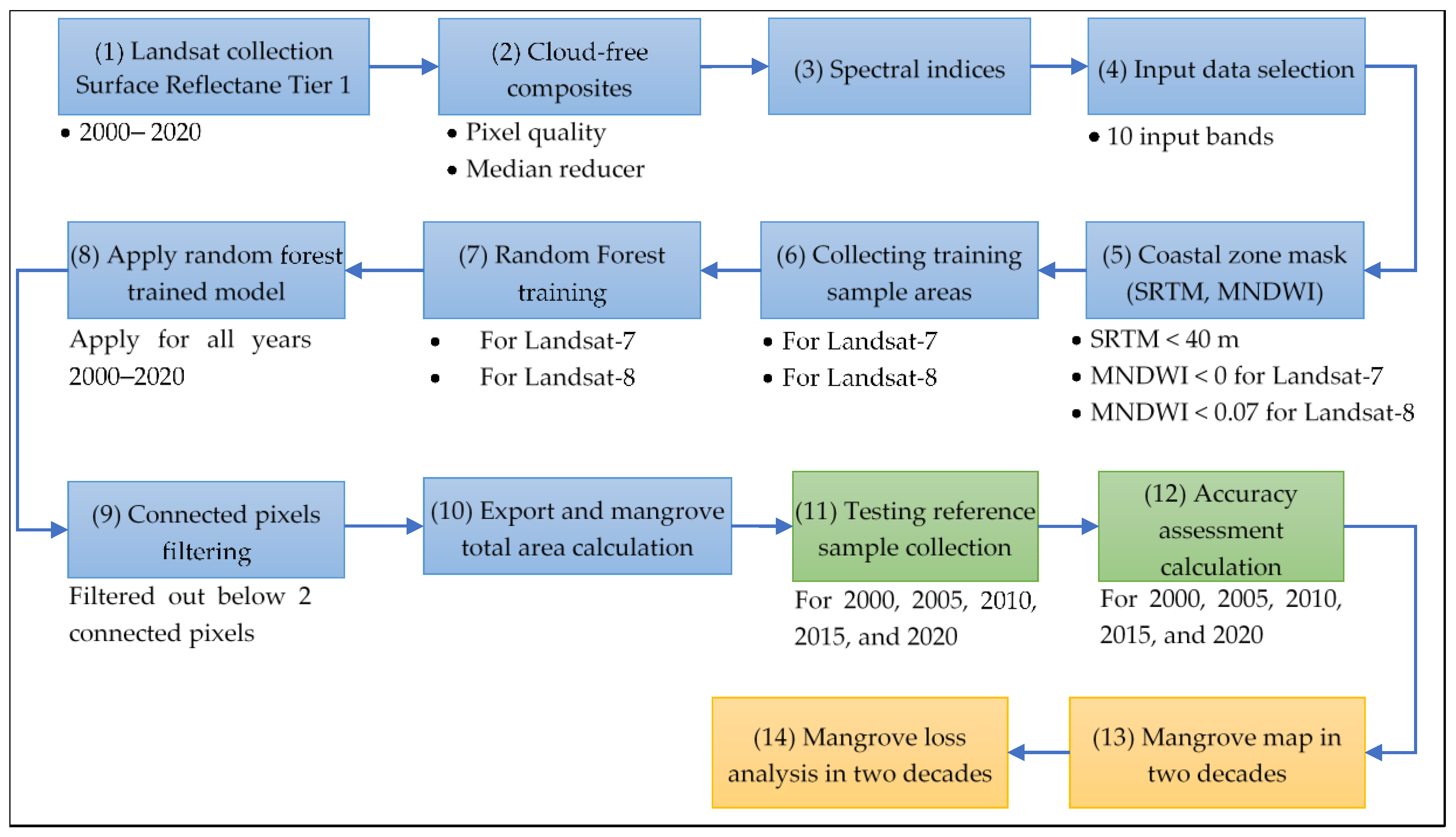
The work stages in this study are divide into data pre-processing, RF training, mangrove mapping, accuracy assessment, and mangrove loss analysis. The research workflow for this study is shown in Figure 2. The pre-processing step completed on GEE and included Landsat-7 and 8 SR collection tier 1, cloud free composites processing by using band pixel quality (BQA) and median reducer, spectral indices processing, input data selection, and coastal zone mask by using Shuttle Radar Topography Mission (SRTM) and modified normalized difference water index (MNDWI) (Section 2.3.1). The RF training process included training sample area collection and mangrove mapping in two decades explained in Section 2.3.2. The accuracy assessment calculation uses independent testing reference samples in 2000, 2005, 2010, 2015 and 2020 to calculate the produced map accuracy (Section 2.3.3). While the mangrove loss analysis using the loss rate calculation to know the mangrove loss rate in two decades in the East Luwu coastal zone.

2.3.1. Data Pre-Processing

Data pre-processing have been carried out on the GEE platform. The first pre-processing step is the Landsat-7 and 8 collection surface reflectance tier 1 data by using filter date for 20 years. Starting from 2003, Landsat-7 has scanline error problem which can affect the classification results. Each year in the Landsat collection process is from the first of January to the end of December for every year. The second step of data pre-processing is cloud-free composites. We used the BQA algorithm from GEE to obtain the free-cloud Landsat images and used the median function to obtain the median pixel value from the date range every year. The output from the second step is the final cloud-free Landsat images from 2000 until 2020. The next step is to calculate the spectral indices and combine with the original bands from Landsat (Section 2.2).
The final step of the data pre-processing is coastal zone mask processing. The mangrove area is located in the tidal zone, so the coastal zone masking is important to minimize the error results. The SRTM and MNDWI data were used here to perform the coastal zone masking for each year. Each image with SRTM value less than 40 m will be including as the input data. Furthermore, the MNDWI data was used here to remove the water body area. We used the MNDWI threshold value of 0 for Landsat-7 and 0.7 for Landsat-8 to remove the water body area based on the previous research [30]. The final input images for this study are the images after SRTM and MNDWI processing.

2.3.2. Random Forest

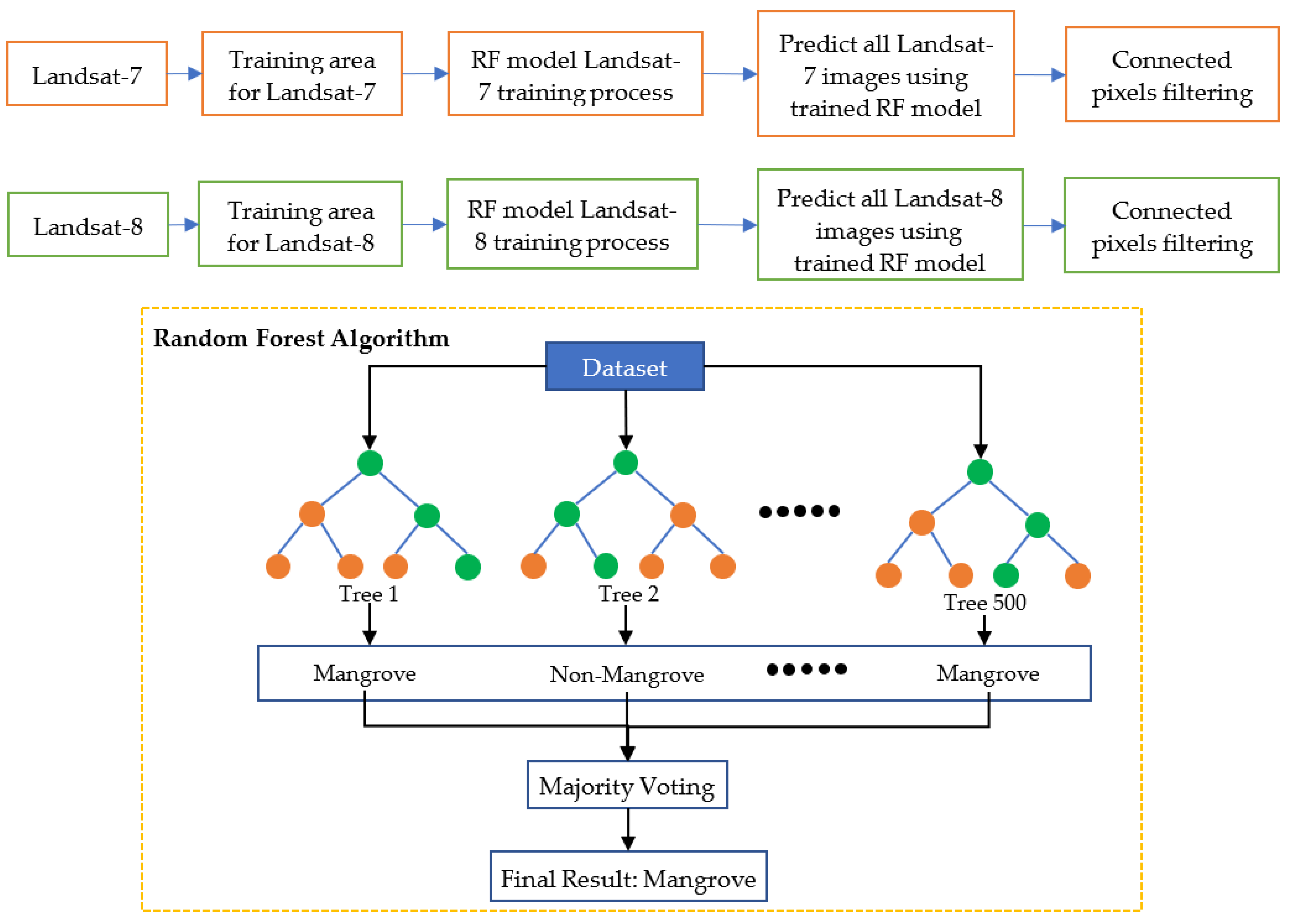
The random forest (RF) training process was carried out on the GEE platform. The RF is tree-based classifier algorithm with more than one total number of trees and uses major voting to predict the final predicted class [31]. Even though GEE provides more than 15 different classifiers, nearly 15,000 papers used the RF algorithm for land use/land cover classification including mangrove mapping in the last 5 years [18]. That’s what made us choose RF as the classifier algorithm for this study. The RF is a tree-based algorithm with more than one decision tree. The RF algorithm for this study and the training process of the RF algorithm is shown in Figure 3. We use a total of 500 trees with two classes (non-mangrove and mangrove) as the predicted output. RF used majority voting to determine the final predicted result from each tree.
In general, the RF training process in this study is divided into two models: (1) the RF model for Landsat-7 and (2) the RF model for Landsat-8 to minimize the effects of difference radiometric resolution of Landsat-7 and Landsat-8. RF is a supervised learning algorithm, so the training data is needed to train the RF algorithm. We collected the training area for the RF algorithm on the GEE platform. We used stratified random sampling around the coastal zone to obtain the training area. We divided the training area for Landsat-7 by using an image in 2000 and the training area for Landsat-8 by using images in 2014 (Figure 4). Then all training areas were converted to the pixel size to obtain the balanced training data. The total training pixels for the Landsat-7 and Landsat-8 are shown in Table 4. For the Landsat-7, the total of training pixels is 8174 with 4152 non-mangrove class and 4022 mangrove class. While the total training pixels for Landsat-8 is 3142 pixels with 1306 non-mangrove class and 1836 pixels for mangrove class. The total training pixel of Landsat-8 is less than Landsat-7 because in 2014 some mangrove areas were already lost.
The RF training process is shown in the top part of Figure 3. The training area from image 2000 was used as the training samples to train the RF model Landsat-7, then the training RF model Landsat-7 was used to predict all Landsat-7 images (2000–2013) and finally the connected pixels filtering was used here to remove non-connected mangrove pixel. The process for the RF model Landsat-8 is the same but uses the training area from image 2014 and predicts all Landsat-8 images (2014–2020). The final result from the RF algorithm is mangrove maps from 2000 to 2020 after the connected pixels filtering process.

2.3.3. Evaluation Assessment

The produced maps from the RF algorithm will be evaluated by using evaluation assessment. The independent testing dataset was collected here to evaluate the produced mangrove maps in the years 2000, 2005, 2010, 2015 and 2020 or every 5 years. The testing dataset was collected based on a new round of stratified random sampling over the same reference images in the years 2000, 2005, 2010, 2015 and 2020 [15]. We collected 250 testing points for the non-mangrove class and 250 testing points for the mangrove class every 5 years. In total, 2500 testing points were collected.
The confusion matrix was used here for the evaluation assessment (Table 5). We calculated 5 confusion matrices for the years 2000, 2005, 2010, 2015 and 2020. The confusion matrix was used here to calculate the user’s accuracy (UA) and producer’s accuracy (PA) for the non-mangrove and mangrove classes. The overall accuracy (OA) is also used here to know the quality of produced maps. Equations (1)–(3) shows the formula to calculate UA, PA, and OA score.
User s   Accuracy   ( UA ) = TN TN + FP
Producer s   Accuracy   ( PA ) = TP TP + FN
Overall   Accuracy   ( OA ) = TP + TN TP + TN + FP + FN

3. Results

This section presents the RF classification results in the years 2000, 2010 and 2015 (Section 3.1). The confusion matrices for the years 2000, 2005, 2010, 2015 and 2020 are also shown in Section 3.1. Based on the evaluation assessment results, the produced maps show good OA scores larger than 0.95. The two decades mangrove loss analysis is explained in Section 3.2.

3.1. Classification Results

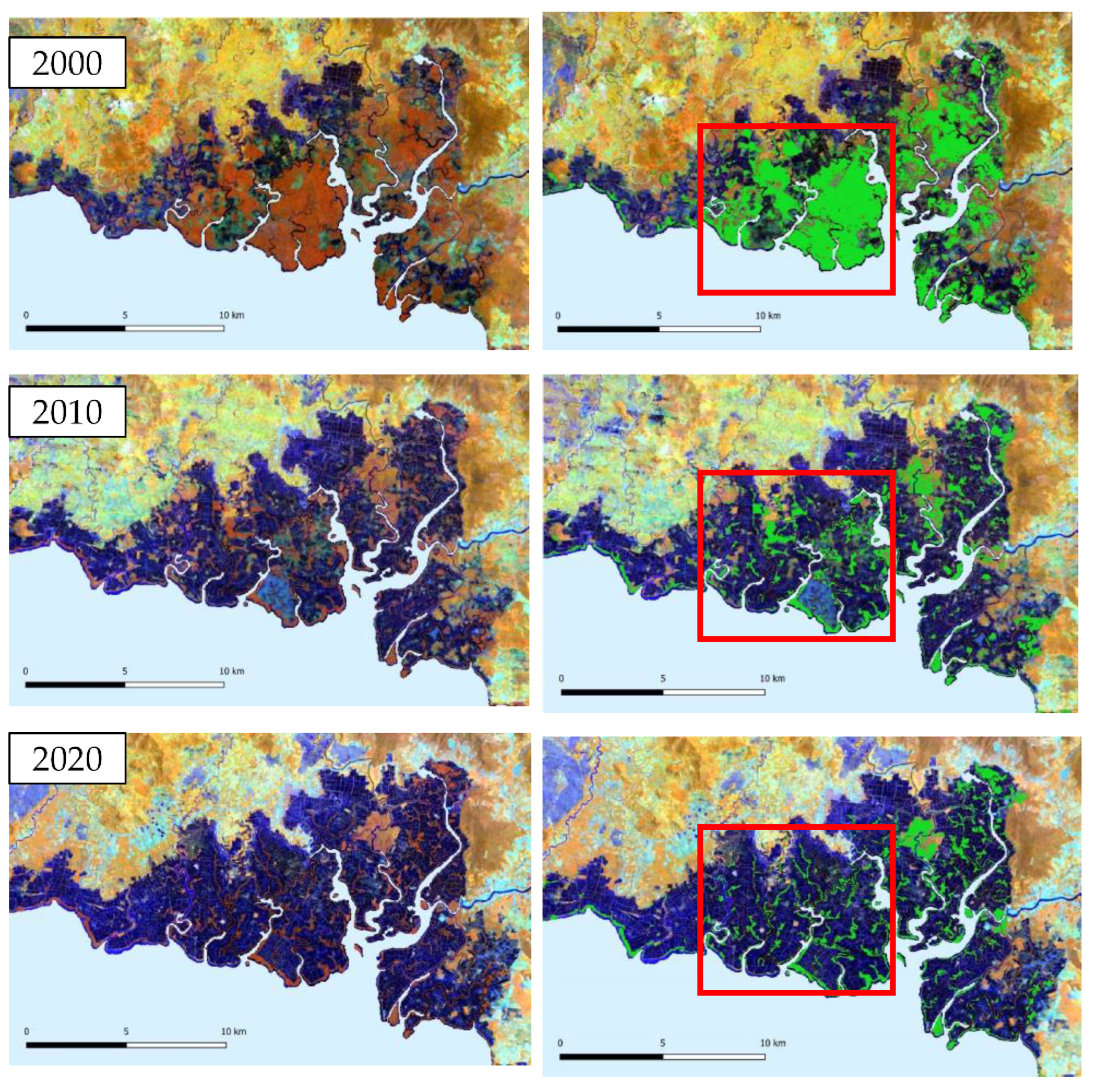
After the RF training process for Landsat-7 and Landsat-8, the trained models were used to predict non-mangrove and mangrove areas in the whole study area for the years 2000 to 2020. The trained Landsat-7 RF model was used to predict non-mangrove and mangrove areas from the years 2000 to 2013, while the trained Landsat-8 RF model was used for the years 2014 to 2020. The visualization result of the mangrove area and Landsat composite (NIR, SWIR 1, Red) every 10 years (2000, 2010 and 2020) are shown in Figure 5. Visually, mangrove objects in Landsat composite (NIR, SWIR 1, Red) will look reddish-orange if we compare them with the other vegetation type.
Based on the visualization classification result, in 2000 almost all of the tidal zone is covered by the mangrove forest and just some areas are already covered by the aquaculture pond. 10 years later in 2010, there is a lot of mangrove forest deforestation, especially in the red box, all of the mangrove forests become non-mangrove (aquaculture pond). While based on the classification visualization result in 2020, the distribution of mangroves is similar to the year 2010, only slight changes occurred in some areas. The comparison analysis based on the visualization results from 2000, 2010 and 2020 shows the highest rate of mangrove deforestation happened between the years 2000 to 2010, while only slight changes happened ten years later (2010 to 2020). There were a lot of mangroves in 2000 and then deforested in 2010 according to the classification result.
The second result of this study is the evaluation assessment to know the quality of classified mangrove and non-mangrove areas. The independent testing samples were collected to perform the evaluation assessment by calculating the OA score, UA score, and PA score. A total of 2500 testing samples were used here from the years 2000, 2005, 2010, 2015 and 2020 to calculate the confusion matrix as shown in Figure 6. In general, the classified maps achieved OA score of more than 0.95 in all 5 years results. The highest OA score is from the year 2000 (0.982), while the lowest OA score is from the year 2005 (0.954). The reason why the 2000 classified result has the highest OA score is the trained model using the training data from the year 2000.
Based on all confusion matrices the UA score and PA score of the non-mangrove class is higher than the mangrove class. These results indicate the mangrove class is more difficult to identify than the non-mangrove class. The lowest UA score for the mangrove class is in the year 2005 (0.908), while the highest UA score for the mangrove class is in the year 2000 (0.982). In general, the classified maps from the trained RF model produced acceptable non-mangrove and mangrove maps based on the evaluation assessments.

3.2. Mangroves Loss Monitoring

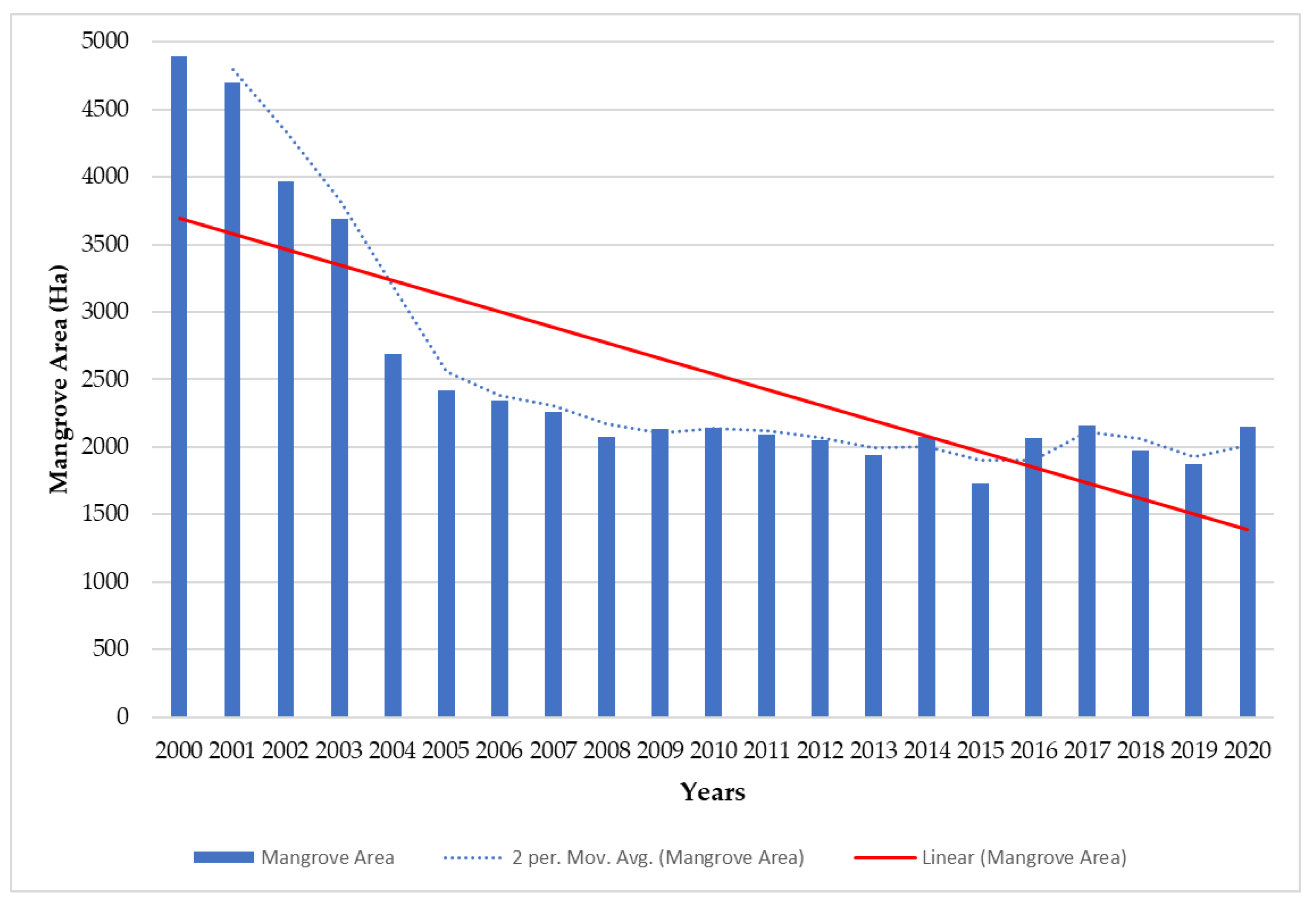
The two decades (2000 to 2020) mangrove loss monitoring in this study is based on produced mangrove maps using an RF algorithm. The results of observations were carried out by looking at changes in the mangrove areas every year. The spatial distribution of the mangrove area shows a change in the location of the mangrove area from 2000 to 2020. Based on the produced mangrove maps every year, the total area of mangroves in two decades is shown in Figure 7. The largest total mangrove area in East Luwu was found in the year 2000 with a total mangrove area of 4895.26 Ha. While the lowest total mangrove area was found in the year 2015 with a total mangrove area of 1730.24 Ha. Based on the linear trendline (red line), the total area of mangroves in East Luwu from 2000 to 2020 has a decreased trend. The most significant decrease occurred in the years 2000–2005. After 2005, there was a narrowing of the fluctuating mangrove areas. The moving average line shows the high deforested mangrove area from 2000 to 2005, then after 2005 become more stable. In 2020 we can find a slight increase in mangrove area compared with the previous year. Based on the linear trendline and moving average line, the status and condition of mangrove forest in East Luwu from 2000 to 2020 tends to decrease.
The result of the intact and loss mangrove area in 2000 to 2020 is shown in Figure 8. The highest mangrove deforestation area can be seen in the orange zoom box. Based on observations of the spatial distribution of the front area is dominated by intact mangrove areas and changes in the mangrove area in 2000 and 2020 are behind it. The shrinkage of mangrove area based on the distribution in 2000 was influenced by changes in land use in the East Luwu area to become a pond area. Intact mangroves in the foreground are used to protect coastlines and aquaculture areas. The addition of mangrove areas in 2020 is outside the mangrove area in 2000 and has a narrow distribution. Based on the results of the distribution on the map, it is known that the narrowing of the mangrove area is behind intact mangroves and is influenced by changes in land use into pond areas.

4. Discussion

The study area of this research is located in the East Luwu, Indonesia with high rate of mangrove deforestation around the study area [12]. Time-series Landsat-7 and Landsat-8 images were used here to produce mangrove map in two decades (2000 to 2020). While RF algorithm was used here as the classifier function in the GEE platform. The trained RF model from the year 2000 (Landsat-7) was used to produce mangrove maps from 2000 to 2013, while the trained RF model from the year 2014 (Landsat-8) was used to produce mangrove maps from 2014 to 2020. The OA score, UA score, and PA score from the evaluation assessment using the independent testing dataset are shown in Table 6. The average OA score from the produced maps (2000, 2005, 2010, 2015 and 2020) is 0.966, while the UA score for the mangrove class is lower than the non-mangrove class but still acceptable. The produced mangrove map using RF trained model achieved good results in terms of accuracy matrices. Based on these results, we assumed all the produced mangrove maps every year can be used for mangrove monitoring analysis.
We calculated the mangrove loss rate percentage per year for every 5 years for further analysis (Table 7). The calculation of mangrove loss rate in this study is based on previous research with following equations [32]:
r = ( 1 t 2 t 1 ) × ln ( A 2 A 1 )
where A1 and A2 are the forest cover at time t1 and t1, respectively. The unit for the annual rate is per year or percentage per year.The first-half first decade (2000 to 2005) has the greatest annual mangrove loss rate among others. The mangrove loss rate in the first-half first decade is −14.11% with the total loss of mangrove area of 2477.39 Ha. This result revealed massive mangrove deforestation in East Luwu from 2000 to 2005. The main factor is the conversion from mangrove areas to aquaculture ponds which happened a lot from 2000 to 2005.
The second-half first decade (2006 to 2010), revealed mangrove loss rate of −2.24% per year with a total loss of mangrove area of 201.51 Ha. The mangrove loss rate in the second-half first decade is not really high as in the first-half decade. While the mangrove loss rate in the first-half second decade (2011 to 2015) increased from the second-half first decade. The mangrove loss rate from the first-half second decade is −4.75% with the total mangrove deforestation area of 362.40 ha, which differs from the previous 5 years by 160.88 Ha. From 2006 to 2015 we found fewer mangrove areas were deforested compared with the first-half first decade (2000 to 2005). The trendline analysis in Figure 7 also shows the narrowing of the fluctuating mangrove areas after 2005. Based on our visual analysis, the decreasing mangrove areas from 2006 to 2015 are still mainly influenced by the aquaculture ponds. After 2005, the loss of mangrove areas is not very high, it is related with the regional government regulation (Peraturan Daerah Luwu Timur No. 2 Year 2005: Rencana Pembangunan Jangka Panjang (RPJP) 2005–2025). This regulation mentioned about environmental issues related to aquaculture ponds and land clearing. In addition to that factor, the procurement of new aquaculture pond has also decreased after 2005 based on visual analysis.
While in the last second decade (2016 to 2020), we found a positive loss rate (+1.04%) percentage which means there is an increase in the total mangrove area in the study area. The total increased mangrove areas from 2016 to 2020 is 87.96 Ha, which does not increase too much. We used Landsat-8 (2016 and 2020) and Sentinel-2 data (2020) as a finer spatial resolution for the visual observations. Based on our observations, the slight increase of total mangrove area in the last second decade was mainly caused by the natural restoration of mangrove areas that happened in mangrove areas directly adjacent to water areas (ocean and river). We also found small abandonment aquaculture ponds in 2016 turned back into mangrove areas in 2020. In fact, there is still conversion of mangrove forests into aquaculture ponds from 2016 to 2020.
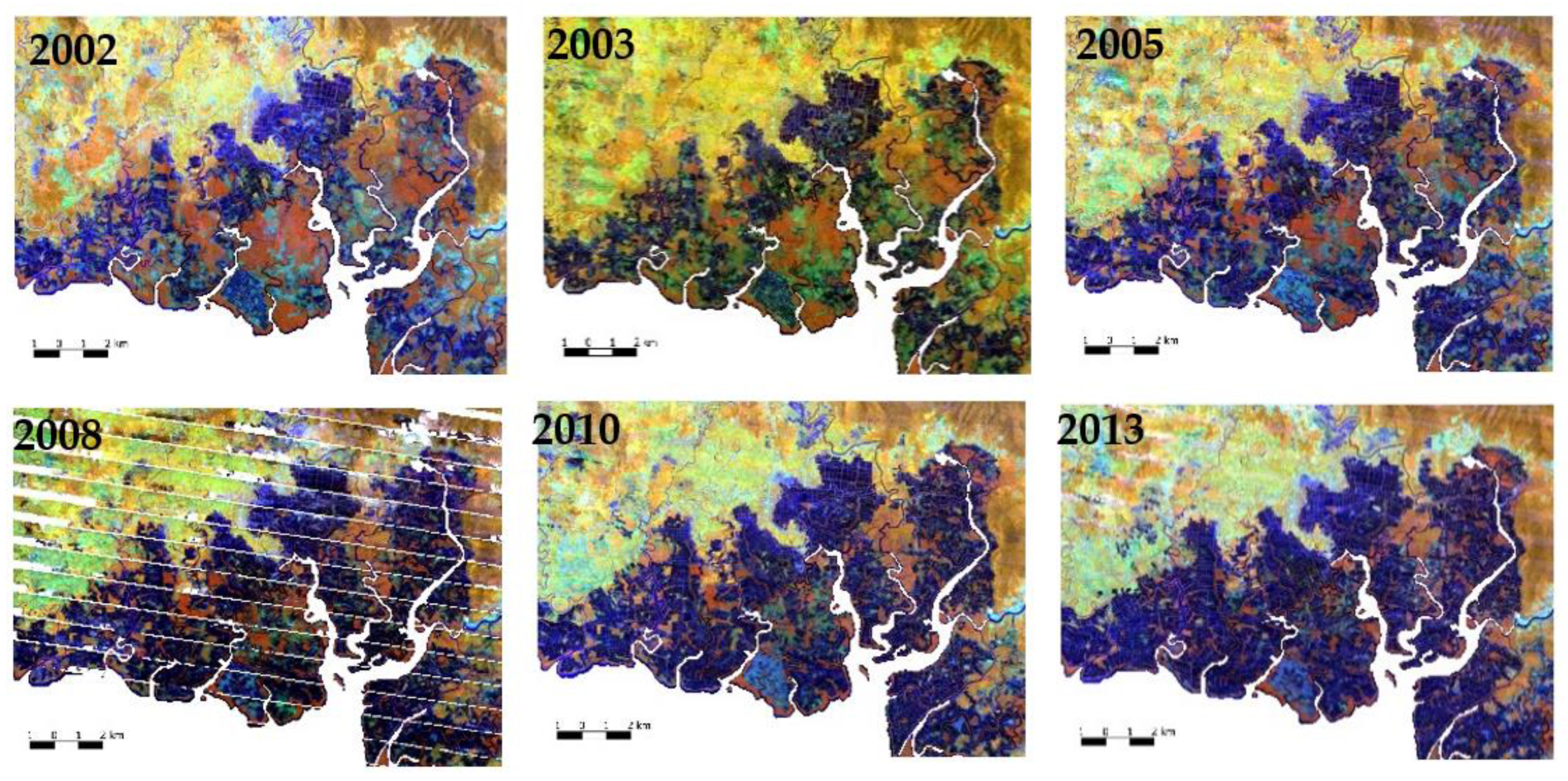
The limitation from the produced mangrove maps in this study is divided into two types. The first type is cloud cover effects in the study area, even though we already used the cloud masking function in the GEE platform, some area still has cloud cover effects. The second type is about scanline error in the Landsat-7 imagery. The scanline errors happened in the Landsat-7 image starting from 2003. We used a median filter from January to December for each year to minimize the scanline error in the Landsat-7 images. Almost all Landsat-7 data from 2003 to 2013 have small scanline errors so it doesn’t affect the classification results much, just the year 2008 has very huge scanline errors (Figure 9). Therefore, the produced mangrove maps from 2003 to 2013 are still acceptable since they had a small scanline error and achieved a good OA score from the evaluation assessment. We only used Landsat-7 images for the year 2000 to 2013 even though they have scanline errors because we cannot find the Landsat-5 data in our study area after the year 2003. To the best of our knowledge, much Landsat-5 data in the specific region and year is still decentralized and not available in the global database. The scanline errors and cloud cover effects affected the produced mangrove cover maps in the whole study area. Future research needs to pay more attention to the scanline errors of Landsat-7 or uses other satellite imagery.

5. Conclusions

Mangrove monitoring is important information to know the status and condition of mangrove forest. This study used Landsat-7 and Landsat-8 satellite imagery with RF algorithm to produce two decades mangrove loss monitoring in East Luwu, Indonesia from 2000 to 2020. Based on the independent testing points, the average OA score from the produced mangrove map is about 0.966, while the average UA score of mangrove class is 0.936. The total mangrove area from 2000 to 2020 has decreased trend with the highest mangrove deforestation happened from 2000 to 2005 with mangrove loss rate −14.11% per year. This study revealed the mangrove deforestation in East Luwu was mainly caused by the aquaculture pond. In the last 5 years (2016 to 2020), this study found a slight increase in total mangrove area by 1.04% (87.96 Ha). The slight increased mangrove area mainly caused by natural recovery and small abandonment aquaculture ponds in 2016 turned back into mangrove areas.

Author Contributions

Conceptualization, I.J. and Y.-N.C.; data curation S.M.R. and P.M.; methodology, I.J.; result analysis, A.G.A.; validation, S.M.R. and P.M.; supervision, Y.-N.C.; writing—original draft, I.J.; writing—review and editing, Y.-N.C., S.M.R., P.M. and A.G.A. All authors have read and agreed to the published version of the manuscript.

Funding

This research received no external funding.

Institutional Review Board Statement

Not applicable.

Informed Consent Statement

Not applicable.

Data Availability Statement

The Landsat-7 and Landsat-8 images are freely accessible. The produced mangrove maps from 2000 to 2020 in East Luwu and the GEE script codes are available by the request.

Acknowledgments

The authors want to thank the GEE platform for freely provided cloud computing process. We also thank the NASA/USGS for freely provided Landsat-7 and Landsat-8 data.

Conflicts of Interest

The authors declare no conflict of interest.

References

  1. Giri, C.; Pengra, B.; Zhu, Z.; Singh, A.; Tieszen, L.L. Monitoring Mangrove Forest Dynamics of the Sundarbans in Bangladesh and India Using Multi-Temporal Satellite Data from 1973 to 2000. Estuar. Coast. Shelf Sci. 2007, 73, 91–100. [Google Scholar] [CrossRef]
  2. Sahu, S.C.; Kumar, M.; Ravindranath, N.H. Carbon Stocks in Natural and Planted Mangrove Forests of Mahanadi Mangrove Wetland, East Coast of India. Curr. Sci. 2016, 110, 2253–2260. [Google Scholar] [CrossRef]
  3. Pham, T.D.; Yokoya, N.; Bui, D.T.; Yoshino, K.; Friess, D.A. Remote Sensing Approaches for Monitoring Mangrove Species, Structure, and Biomass: Opportunities and Challenges. Remote Sens. 2019, 11, 230. [Google Scholar] [CrossRef] [Green Version]
  4. Shahbudin, S.; Zuhairi, A.; Kamaruzzaman, B.Y. Impact of Coastal Development on Mangrove Cover in Kilim river, Langkawi Island, Malaysia. J. For. Res. 2012, 23, 185–190. [Google Scholar] [CrossRef]
  5. Barua, P.; Rahman, S. Sustainable Livelihood of Vulnerable Communities in Southern Coast of Bangladesh through the Utilization of Mangroves. Asian J. Water Environ. Pollut. 2019, 16, 59–67. [Google Scholar] [CrossRef]
  6. Carugati, L.; Gatto, B.; Rastelli, E.; Martire, M.L.; Coral, C.; Greco, S.; Danovaro, R. Impact of Mangrove Forests Degradation on Biodiversity and Ecosystem Functioning. Sci. Rep. 2018, 8, 13298. [Google Scholar] [CrossRef] [Green Version]
  7. Lovelock, C.E.; McAllister, R.R. ‘Blue Carbon’ Projects for The Collective Good. Carbon Manag. 2013, 4, 477–479. [Google Scholar] [CrossRef]
  8. Sanders, C.J.; Maher, D.T.; Tait, D.R.; Williams, D.; Holloway, C.; Sippo, J.Z.; Santos, I.R. Are Global Mangrove Carbon Stocks Driven by Rainfall? J. Geophys. Res. Biogeosci. 2016, 121, 2600–2609. [Google Scholar] [CrossRef]
  9. Sanderman, J.; Hengl, T.; Fiske, G.; Solvik, K.; Adame, M.F.; Benson, L.; Bukoski, J.J.; Carnell, P.; Cifuentes-Jara, M.; Donato, D.; et al. A global map of mangrove forest soil carbon at 30 m spatial resolution. Environ. Res. Lett. 2018, 13, 055002. [Google Scholar] [CrossRef]
  10. Gillanders, S.N.; Coops, N.C.; Wulder, M.A.; Gergel, S.E.; Nelson, T. Multitemporal Remote Sensing of Landscape Dynamics and Pattern Change: Describing Natural and Anthropogenic Trends. Prog. Phys. Geogr. 2008, 32, 503–528. [Google Scholar] [CrossRef]
  11. Valiela, I.; Bowen, J.L.; York, J.K. Mangrove Forests: One of the World’s Threatened Major Tropical Environments. Bioscience 2001, 51, 807–815. [Google Scholar] [CrossRef] [Green Version]
  12. Hamilton, S.E.; Casey, D. Creation of a High Spatio-Temporal Resolution Global Database of Continuous Mangrove Forest Cover for the 21st Century (CGMFC-21). Glob. Ecol. Biogeogr. 2016, 25, 729–738. [Google Scholar] [CrossRef]
  13. Spalding, M.; Kainuma, M.; Collins, L. World Atlas of Mangroves; Earthscan: London, UK, 2010. [Google Scholar]
  14. Primavera, J.H. Development and conservation of Philippine mangroves: Institutional issues. Ecol. Econ. 2000, 35, 91–106. [Google Scholar] [CrossRef]
  15. Richards, D.R.; Friess, D.A. Rates and Drivers of Mangrove Deforestation in Southeast Asia, 2000-2012. Proc. Natl. Acad. Sci. USA 2016, 113, 344–349. [Google Scholar] [CrossRef] [Green Version]
  16. Heumann, B.W. Satellite Remote Sensing of Mangrove Forests: Recent Advances and Future Opportunities. Prog. Phys. Geogr. 2011, 35, 87–108. [Google Scholar] [CrossRef]
  17. Kamal, M.; Farda, N.M.; Jamaluddin, I.; Parela, A. A Preliminary Study on Machine learning and Google Earth Engine for Mangrove Mapping. IOP Conf. Ser. Earth Environ. Sci. 2019, 500, 012038. [Google Scholar] [CrossRef]
  18. Diniz, C.; Cortinhas, L.; Nerino, G.; Rodrigues, J.; Sadeck, L.; Adami, M.; Souza-Filho, P.W.M. Brazilian Mangrove Status: Three Decades of Satellite Data Analysis. Remote Sens. 2019, 11, 808. [Google Scholar] [CrossRef] [Green Version]
  19. Mondal, P.; Liu, X.; Fatoyinbo, T.E.; Lagomasino, D. Evaluating Combinations of Sentinel-2 Data and Machine-Learning Algorithms for Mangrove Mapping in West Africa. Remote Sens. 2019, 11, 2928. [Google Scholar] [CrossRef] [Green Version]
  20. Gorelick, N.; Hancher, M.; Dixon, M.; Ilyushchenko, S.; Thau, D.; Moore, R. Google Earth Engine: Planetary-scale geospatial analysis for everyone. Remote Sens. Environ. 2017, 202, 18–27. [Google Scholar] [CrossRef]
  21. Waluyo, W.; Arifin, T.; Yonvitner, Y.; Riani, E. Rumput Laut; Potensi Perairan Kabupaten Luwu Dan Kota Palopo, Teluk. Bone, Sulawesi Selatan; Plantaxia: Yogyakarta, Indonesia, 2017. [Google Scholar]
  22. Pariwono, J.I. Australian Co-Operative Programmes in Marine Sciences: Tides and Tidal Phenomena in the ASEAN Region; Flinders University of South Australia: Queensland, Australia, 1985. [Google Scholar]
  23. Worthington, T.A.; zu Ermgassen, P.S.E.; Friess, D.A.; Krauss, K.W.; Lovelock, C.E.; Thorley, J.; Tingey, R.; Woodroffe, C.D.; Bunting, P.; Cormier, N.; et al. A global biophysical typology of mangroves and its relevance for ecosystem structure and deforestation. Sci. Rep. 2020, 10, 14652. [Google Scholar] [CrossRef]
  24. Kusmana, C. Distribution and Current Status of Mangrove Forests in Indonesia. In Mangrove Ecosystems of Asia; Faridah-Hanum, I.A.L., Hakeem, K.R., Munir, O., Eds.; Springer: New York, NY, USA, 2014; pp. 37–60. ISBN 9781461485827. [Google Scholar]
  25. Sribianti, I. Valuasi Ekonomi Hutan Mangrove: Studi Kasus Valuasi Ekonomi Kawasan Hutan Mangrove Malili Kabupaten Luwu Timur. J. Sains. Teknol. 2008, 8, 186–192. [Google Scholar]
  26. Jamaluddin, I.; Thaipisutikul, T.; Chen, Y.-N.; Chuang, C.-H.; Hu, C.-L. MDPrePost-Net: A Spatial-Spectral-Temporal Fully Convolutional Network for Mapping of Mangrove Degradation Affected by Hurricane Irma 2017 Using Sentinel-2 Data. Remote Sens. 2021, 13, 5042. [Google Scholar] [CrossRef]
  27. Tucker, C.J. Red and photographic infrared linear combinations for monitoring vegetation. Remote Sens. Environ. 1979, 8, 127–150. [Google Scholar] [CrossRef] [Green Version]
  28. Gupta, K.; Mukhopadhyay, A.; Giri, S.; Chanda, A.; Datta Majumdar, S.; Samanta, S.; Mitra, D.; Samal, R.N.; Pattnaik, A.K.; Hazra, S. An index for discrimination of mangroves from non-mangroves using LANDSAT 8 OLI imagery. MethodsX 2018, 5, 1129–1139. [Google Scholar] [CrossRef]
  29. Shi, T.; Liu, J.; Hu, Z.; Liu, H.; Wang, J.; Wu, G. New spectral metrics for mangrove forest identification. Remote Sens. Lett. 2016, 7, 885–894. [Google Scholar] [CrossRef]
  30. Zhai, K.; Wu, X.; Qin, Y.; Du, P. Comparison of surface water extraction performances of different classic water indices using OLI and TM imageries in different situations. Geo-Spat. Inf. Sci. 2015, 18, 32–42. [Google Scholar] [CrossRef]
  31. Breiman, L. Random Forests. Mach. Learn. 2001, 45, 5–32. [Google Scholar] [CrossRef] [Green Version]
  32. Puyravaud, J.-P. Standardizing the calculation of the annual rate of deforestation. For. Ecol. Manag. 2002, 177, 593–596. [Google Scholar] [CrossRef]
Figure 1. Study area for this research located in the East Luwu (Luwu Timur), Indonesia.
Geomatics 02 00016 g001
Figure 2. Research workflow, the blue boxes stand for all processing inside the Google Earth Engine (GEE), while the green and orange boxes stand for all processing in GIS software. SRTM and MNDWI denote Shuttle Radar Topography Mission and Modified Normalize Different Water Index, respectively.
Geomatics 02 00016 g002
Figure 3. Random forest algorithm for this study.
Geomatics 02 00016 g003
Figure 4. Distribution of training area for random forest algorithm in Landsat-7 and Landsat-8.
Geomatics 02 00016 g004
Figure 5. Visualization results in year 2000, 2010 and 2020. The left column is Landsat composite images (NIR, SWIR 1, Red) and the right column is Landsat image with the classified mangrove area (green color).
Geomatics 02 00016 g005
Figure 6. Confusion matrix result from independent reference testing points in 2000, 2005, 2010, 2015 and 2020. N-Mg, Mg, UA, and PA stand for non-mangrove class, mangrove class, user’s accuracy, and producer’s accuracy, respectively. The blue color in the confusion matrix tables is true positive and true negative, while the orange box is overall accuracy.
Geomatics 02 00016 g006
Figure 7. Mangrove area loss monitoring from 2000 to 2020 in East Luwu.
Geomatics 02 00016 g007
Figure 8. Intact and loss mangrove map from 2000 until 2020. Intact mangrove is the mangrove area in 2000 and still intact in 2020, Mangroves in 2020 is the mangrove area that just existed in 2020, and Mangroves in 2000 is the mangrove areas that existed in 2000 then deforested in 2020.
Geomatics 02 00016 g008
Figure 9. The effects of scanline errors in the Landsat-7 imagery.
Geomatics 02 00016 g009
Table 1. Characteristics of Landsat-7 ETM+ and Landsat-8 OLI and TIRS.
Landsat-7Landsat-8 OLI
BandsWavelength (μm)Resolution (m)BandsWavelength (μm)Resolution (m)
Band 1—Aerosol0.43–0.4530
Band 1—Blue0.45–0.5230Band 2—Blue0.45–0.5130
Band 2—Green0.52–0.6030Band 3—Green0.53–0.5930
Band 3—Red0.63–0.6930Band 4—Red0.64–0.6730
Band 4—NIR0.77–0.9030Band 5—NIR0.85–0.8830
Band 5—SWIR 11.55–1.7530Band 6—SWIR 11.57–1.6530
Band 6—Thermal10.40–12.5060 (30)Band 7—SWIR 22.11–2.2930
Band 7—SWIR 22.09–2.3530Band 8—Pan0.50–0.6815
Band 8—Pan0.52–0.9015Band—9 Cirrus1.36–1.3830
Band 10—THERMAL 110.6–11.19100 (30)
Band 11—Thermal 211.50–12.51100 (30)
Table 2. Spectral indices formula.
Spectral IndicesFormulaReferences
NDVI ( NIR RED ) ( NIR + RED ) [27]
CMRI(NDVI−NDWI)[28]
NDMI ( SWIR 2 Green ) ( SWIR 2 + Green ) [29]
MMRI ( | MNDWI | | NDVI | ) ( | MNDWI | + | NDVI | ) [18]
Table 3. Input Landsat images for two decades analysis.
YearImagesYearImages
2000Landsat-72011Landsat-7
2001Landsat-72012Landsat-7
2002Landsat-72013Landsat-7
2003Landsat-72014Landsat-8
2004Landsat-72015Landsat-8
2005Landsat-72016Landsat-8
2006Landsat-72017Landsat-8
2007Landsat-72018Landsat-8
2008Landsat-72019Landsat-8
2009Landsat-72020Landsat-8
2010Landsat-7
Table 4. Total training pixels for Landsat-7 and Landsat-8.
ImagesYearNon-Mangrove MangroveTotal Pixels
Landsat-72000415240228174
Landsat-82014130618363142
Table 5. Confusion matrix for evaluation assessment.
Reference Data
Predicted Result MangroveNon-Mangrove
MangroveTrue Positive (TP)False Positive (FP)
Non-MangroveFalse Negative (FN)True Negative (TN)
Table 6. The average of evaluation assessment in the year of 2000, 2005, 2010, 2015 and 2020.
Testing DataOA ScoreUA N-MgUA MgPA N-MgPA Mg
20000.9820.9840.9800.9800.984
20050.9541.0000.9080.9161.000
20100.9700.9960.9440.9470.996
20150.9560.9960.9160.9220.996
20200.9661.0000.9320.9361.000
Average Score0.9660.9950.9360.9400.995
Table 7. Mangrove loss rate percentage per year every 5 years. The “↓” symbol represents the loss trend, while the “↑” symbol represents the gain trend.
YearsTotal Changes Area (Ha)Loss Rate (% per Year)
2000–2005↓ 2477.39−14.11% ↓
2006–2010↓ 201.51−2.24% ↓
2011–2015↓ 362.40−4.75% ↓
2016–2020↑ 87.96+1.04% ↑
Publisher’s Note: MDPI stays neutral with regard to jurisdictional claims in published maps and institutional affiliations.