
Quality Assessment of DJI Zenmuse L1 and P1 LiDAR and Photogrammetric Systems: Metric and Statistics Analysis with the Integration of Trimble SX10 Data


Abstract
:1. Introduction
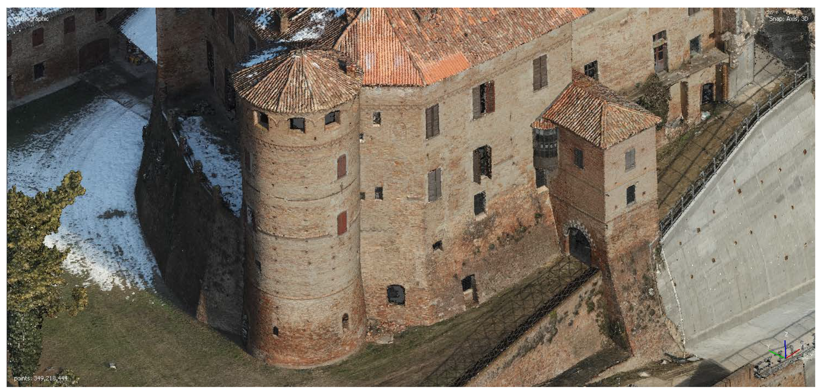
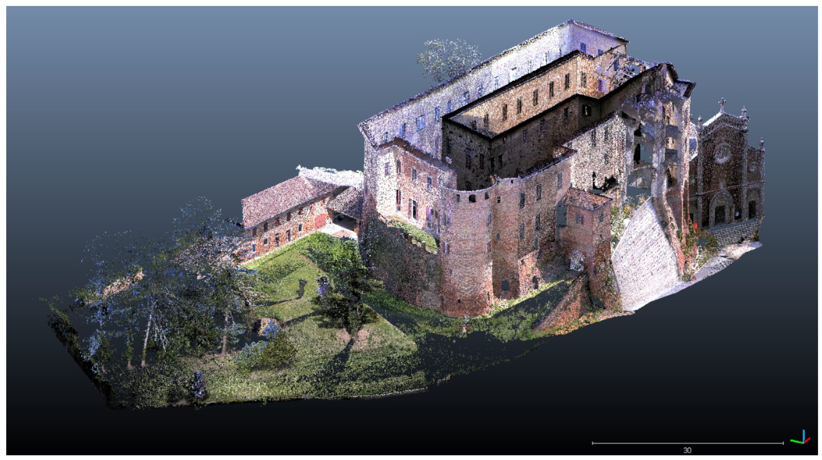
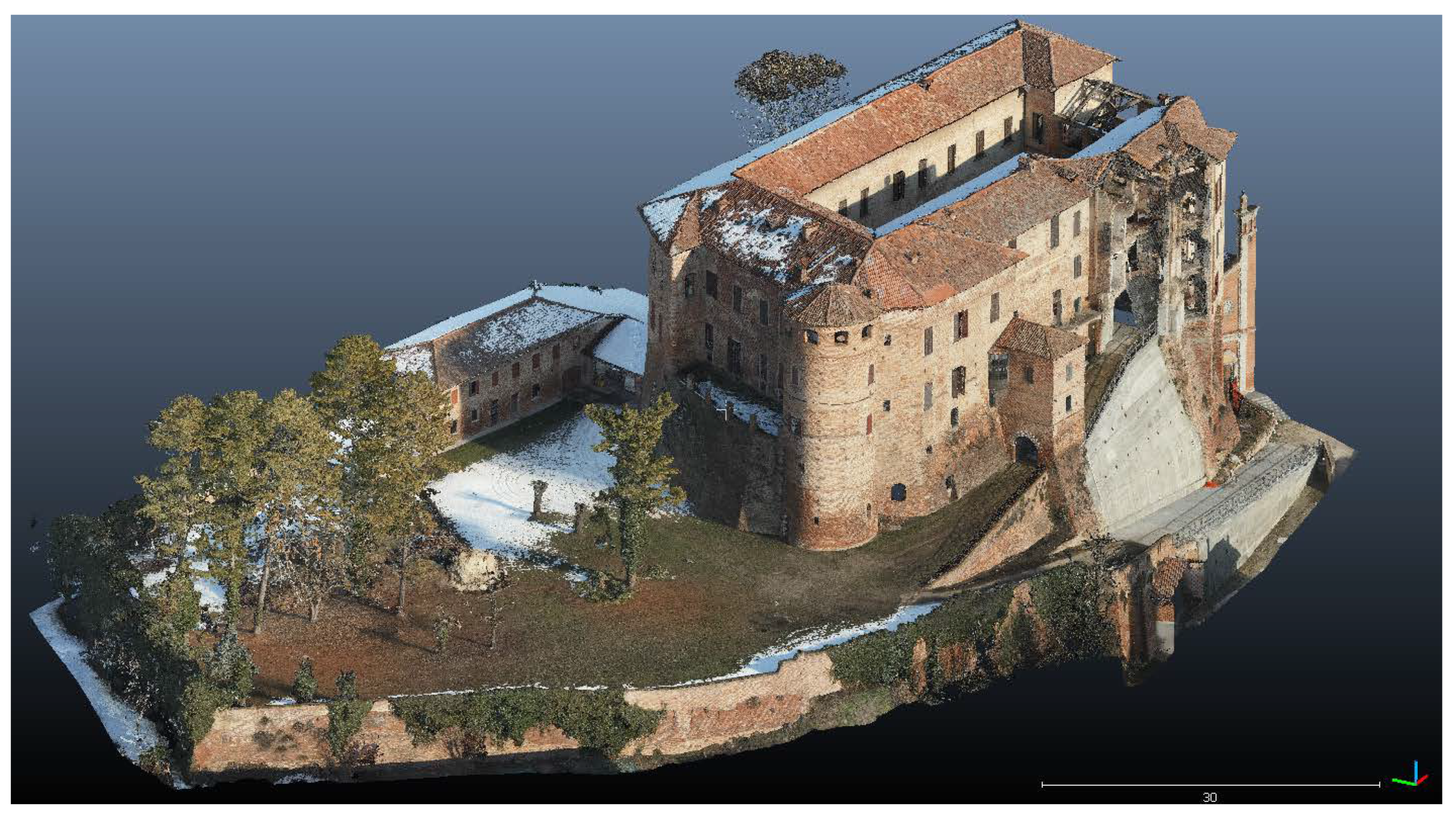
Frinco Castle
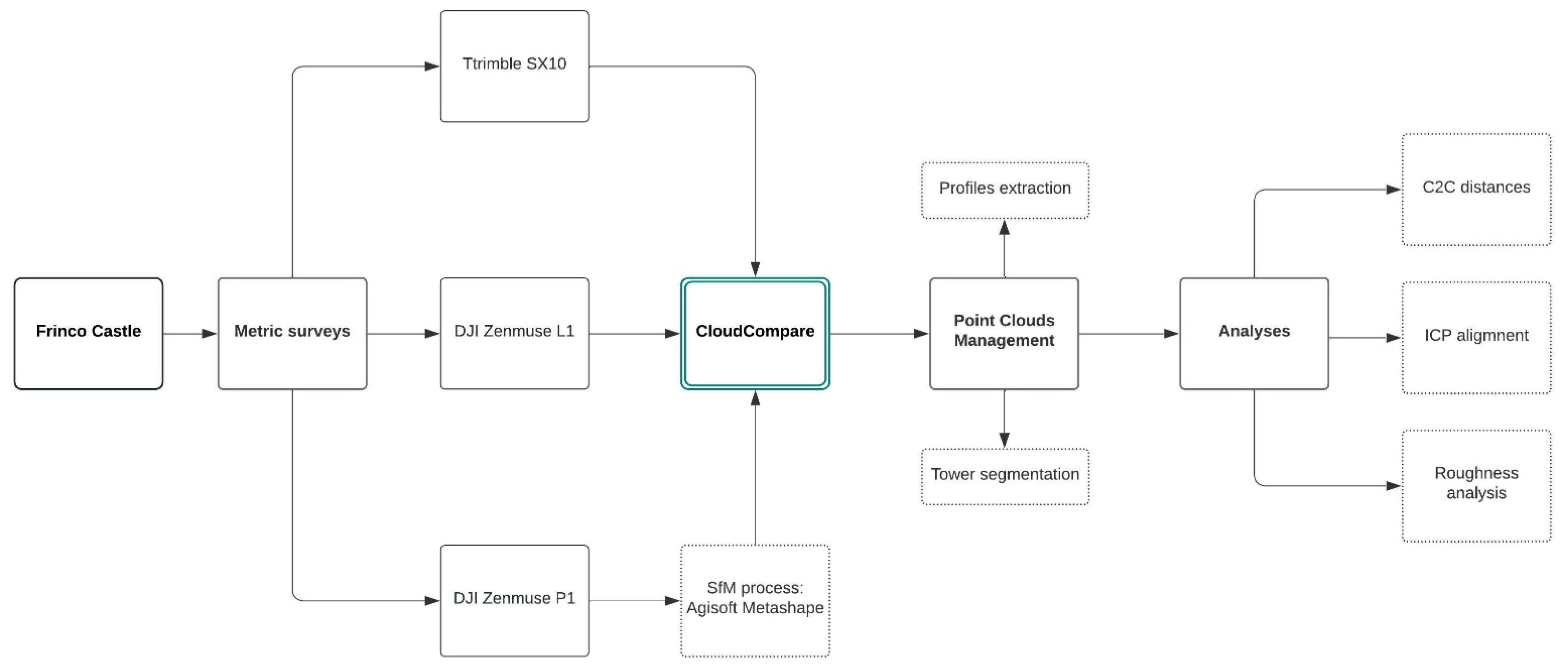
2. Materials and Methods
2.1. DJI Zenmuse L1 Description and Accuracy
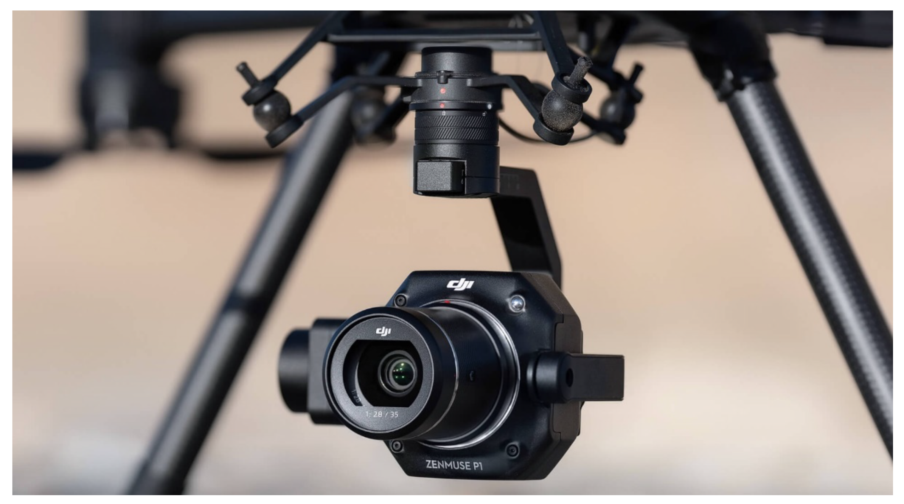
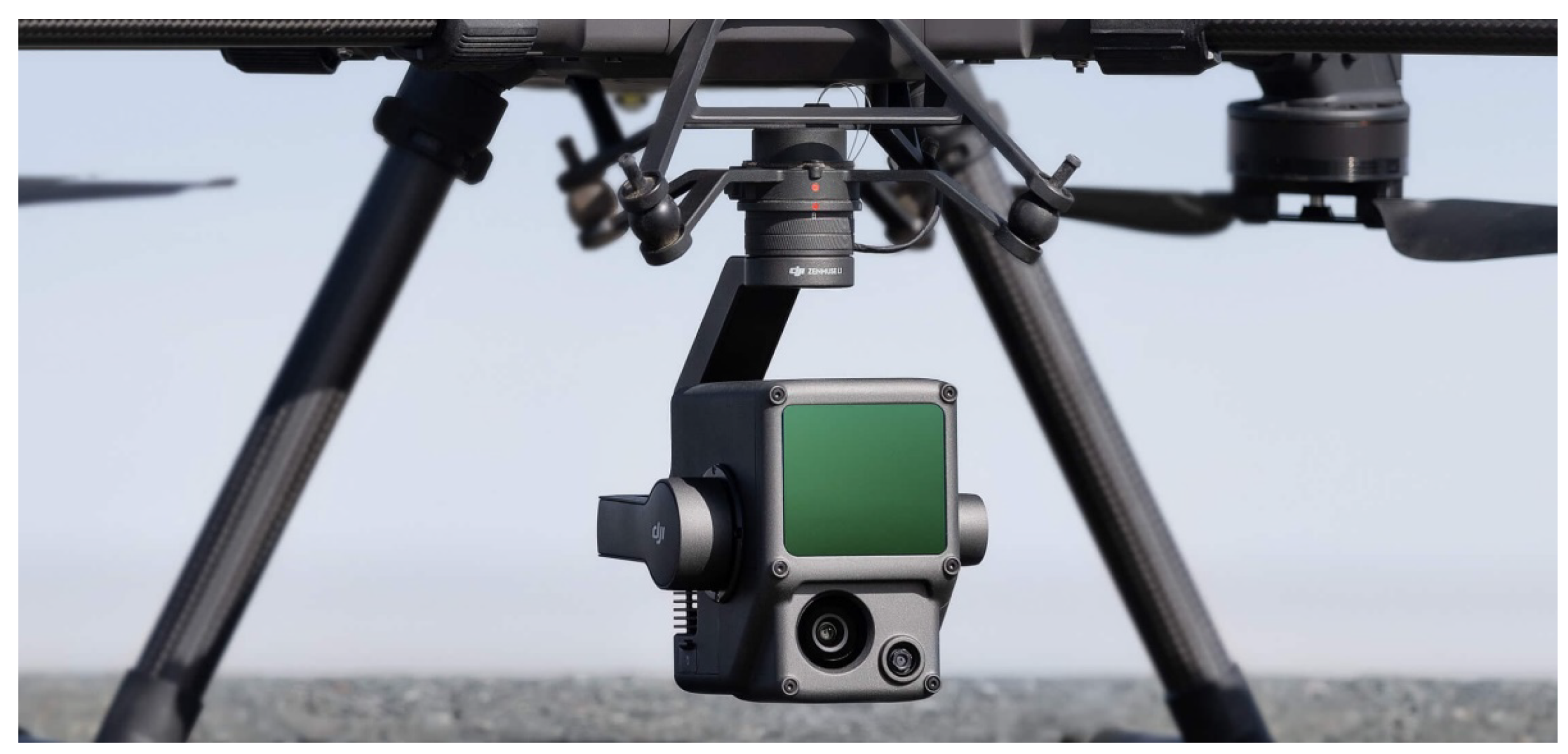
2.2. DJI Zenmuse P1 Description and Accuracy
3. Metric Acquisitions, Data Accuracy and Processing
3.1. Metric Acquisitions: Trimble SX10 and UAS Flights
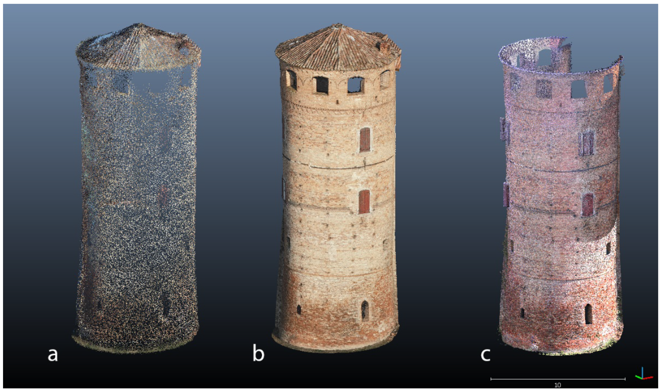
3.2. Zenmuse L1 Data and Accuracy
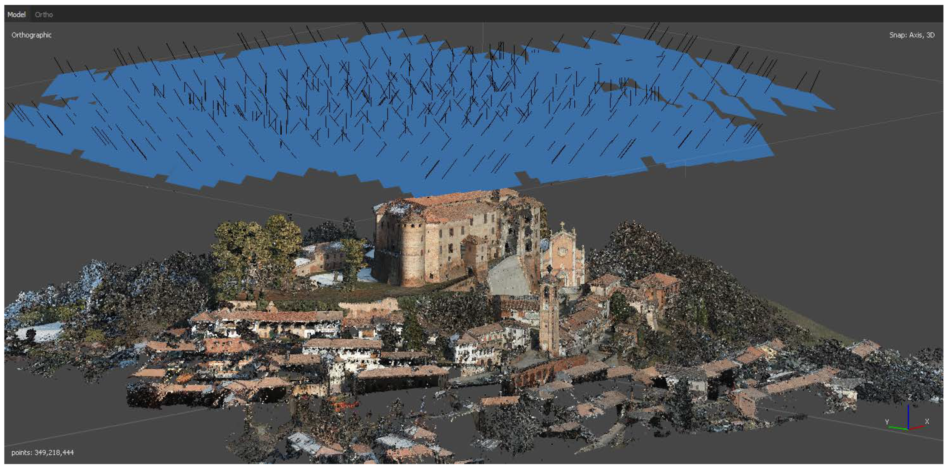
3.3. Zenmuse P1 Data Processing and Accuracy
4. Metric Evaluation and Statistical Analyses of Point Clouds
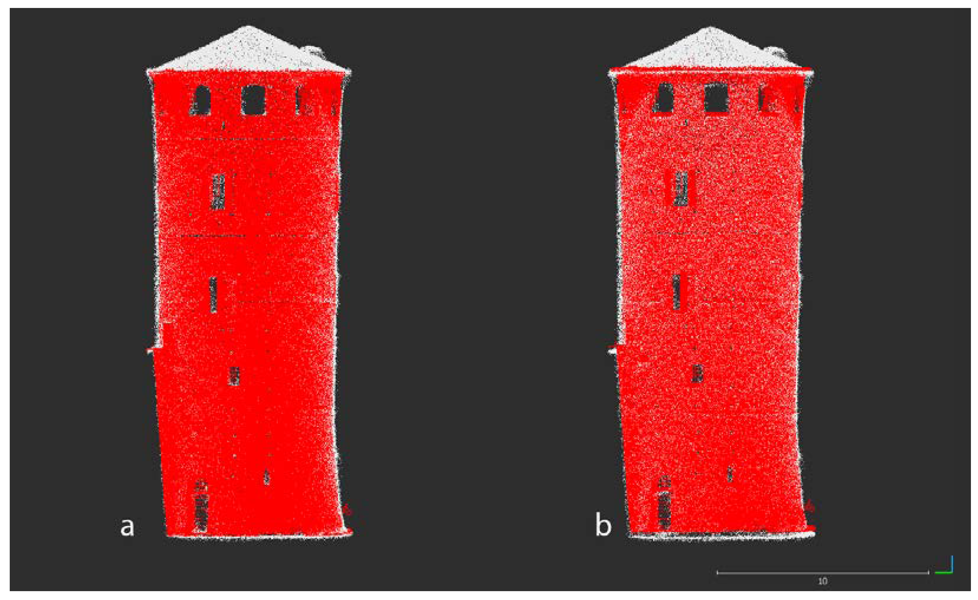
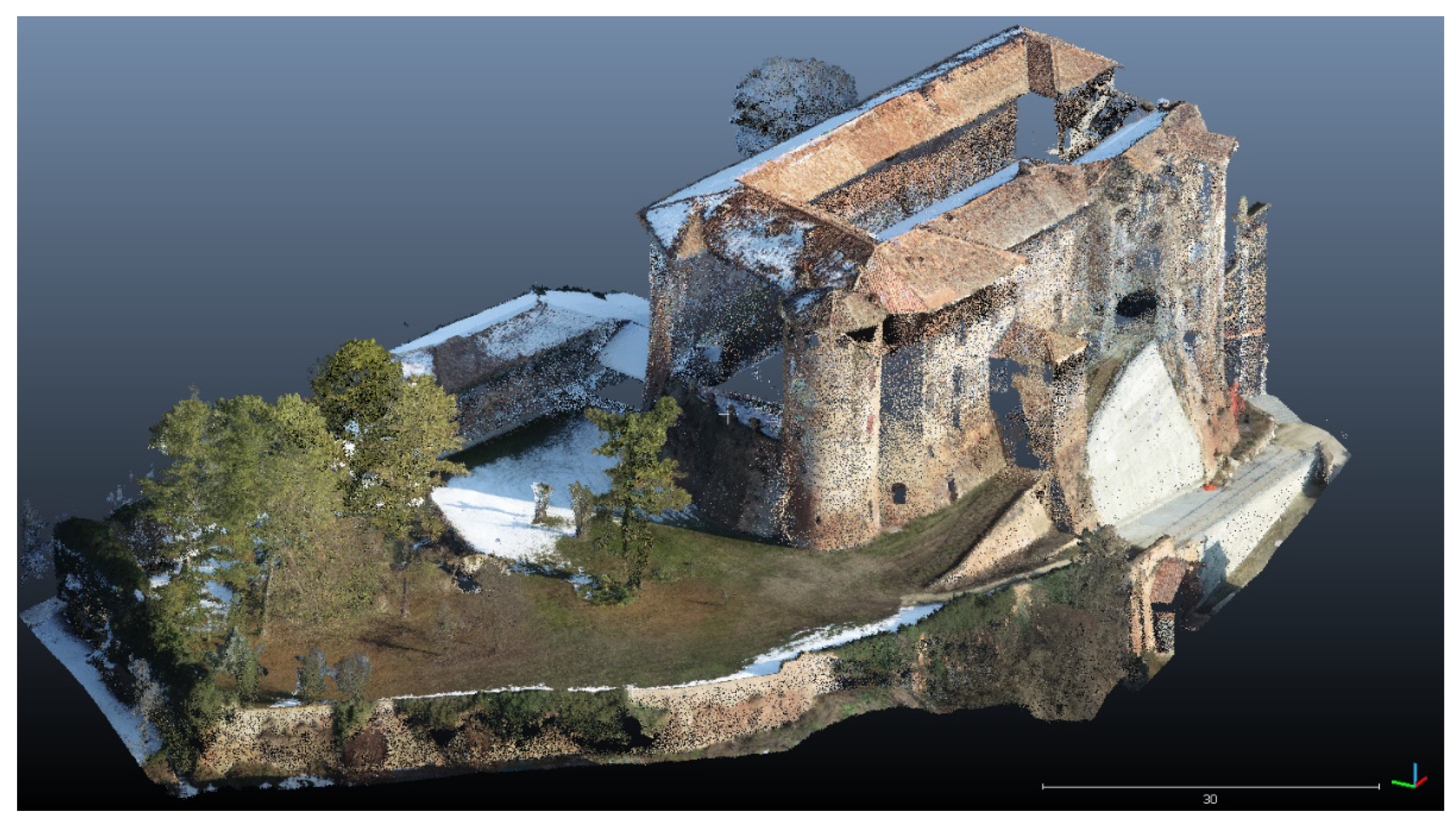
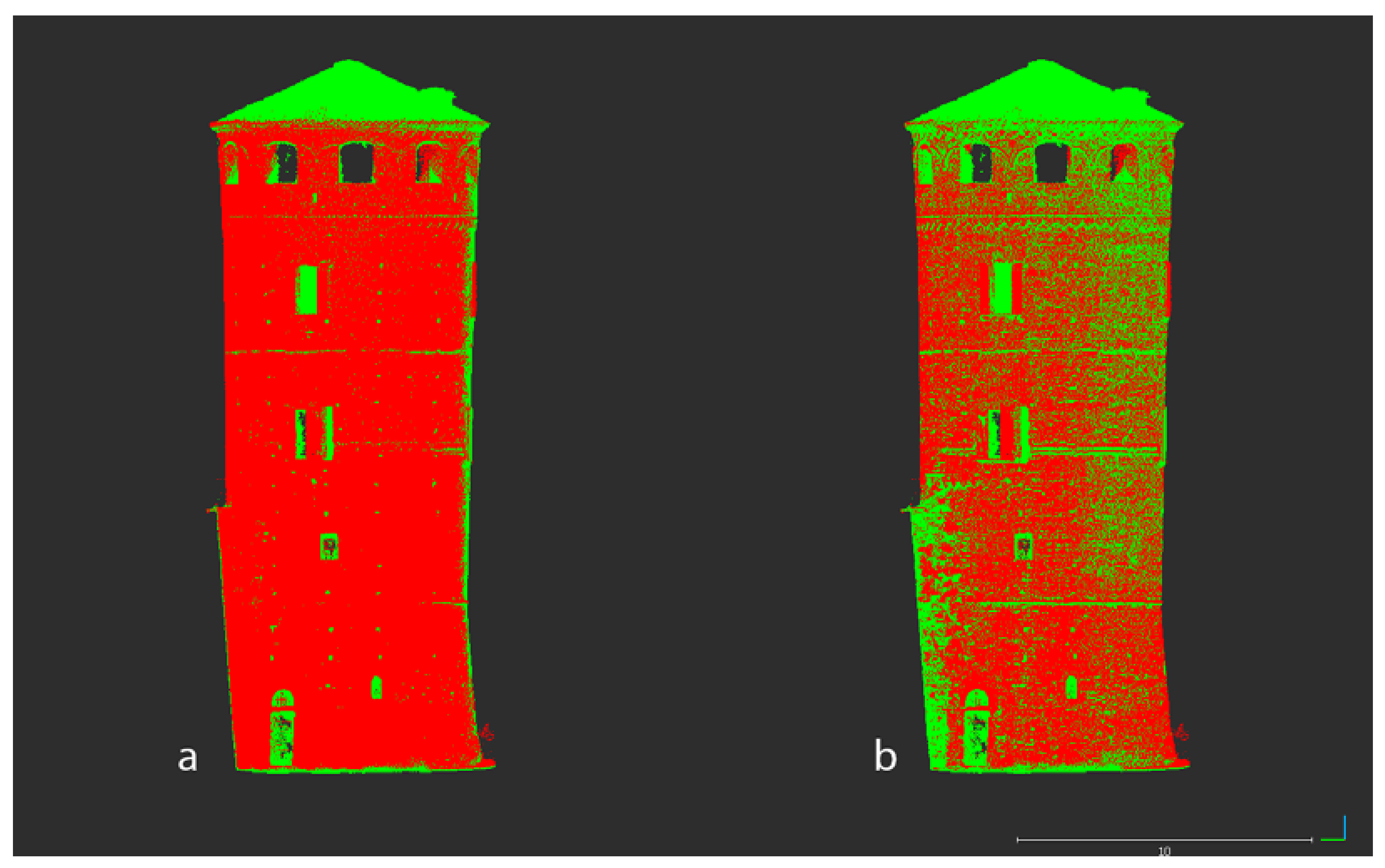
4.1. The Analysis of the Tower of Frinco Castle
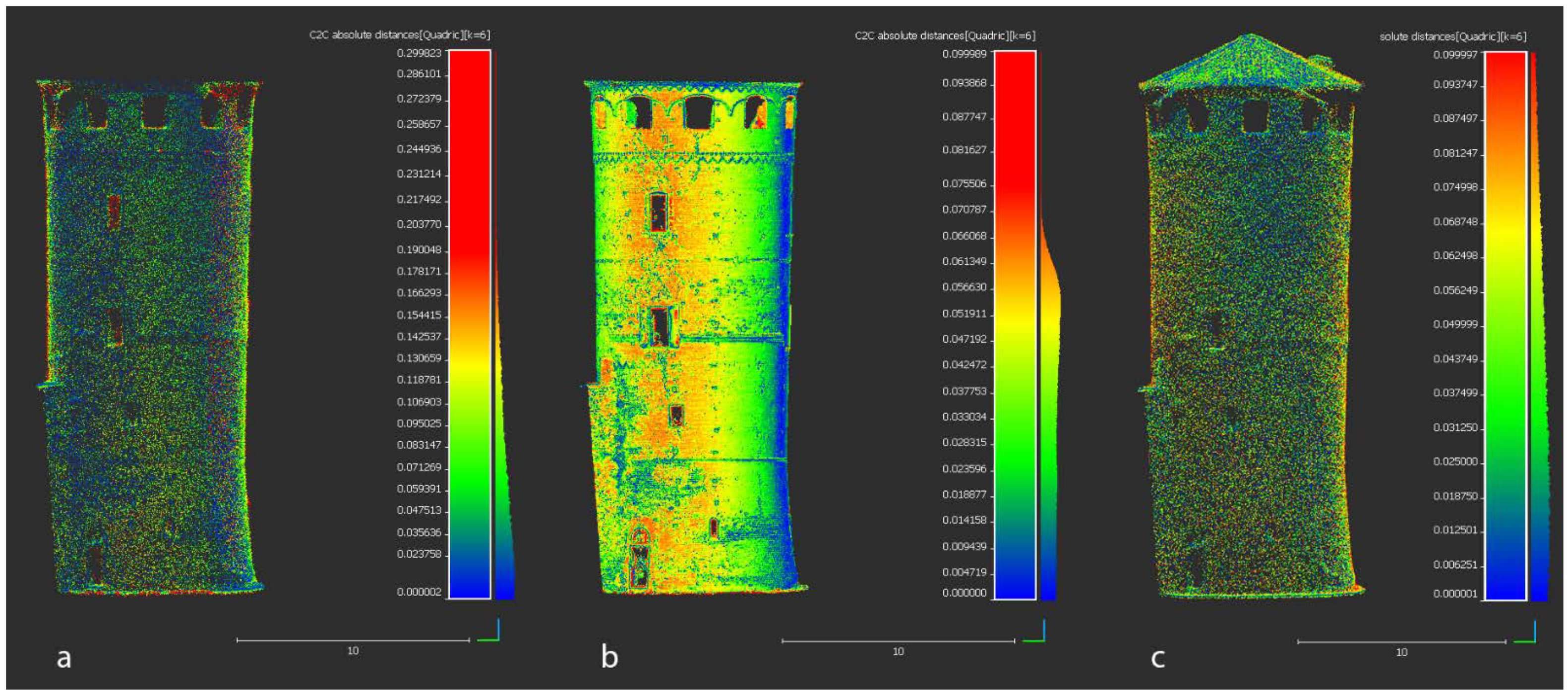
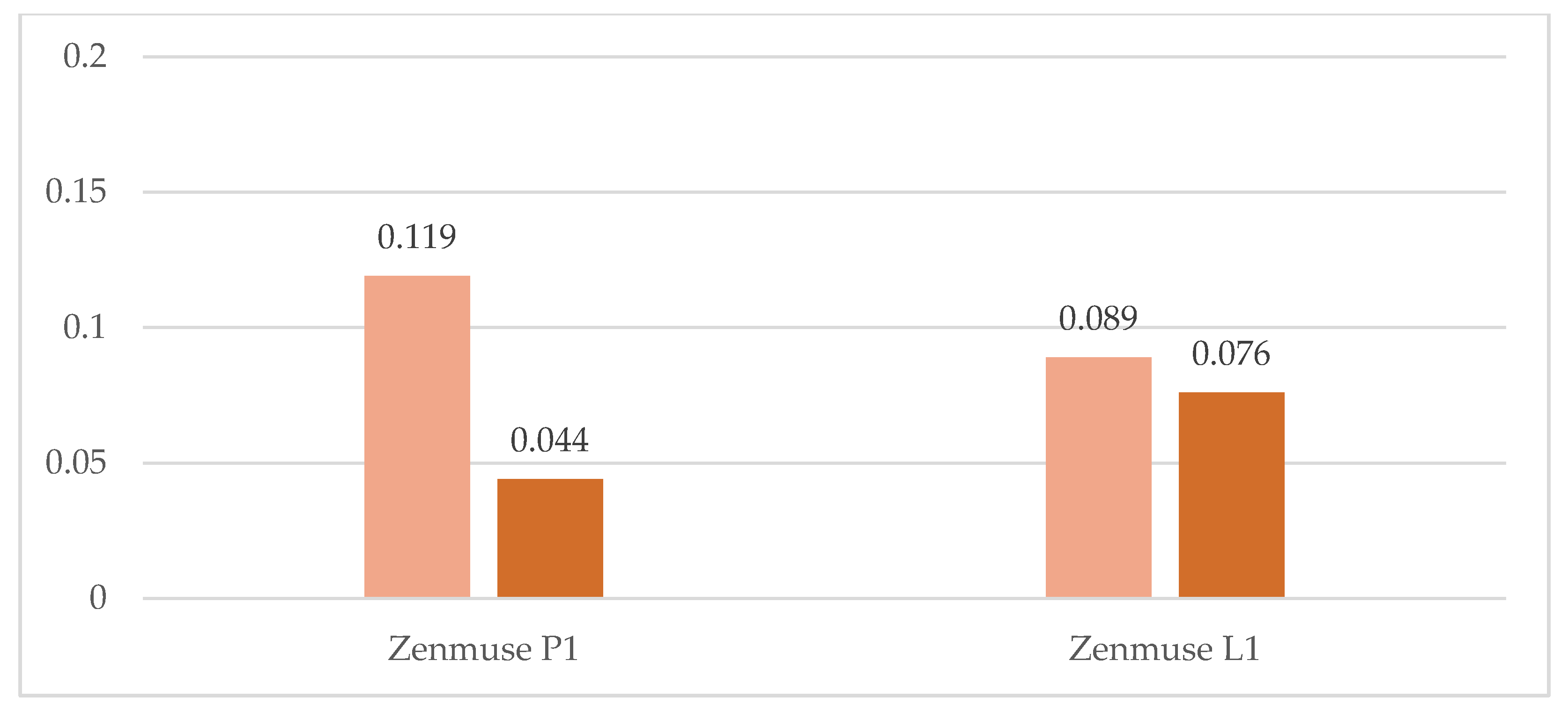
4.1.1. Cloud-to-Cloud Distance (C2C)
4.1.2. ICP Fine Registration and Alignment
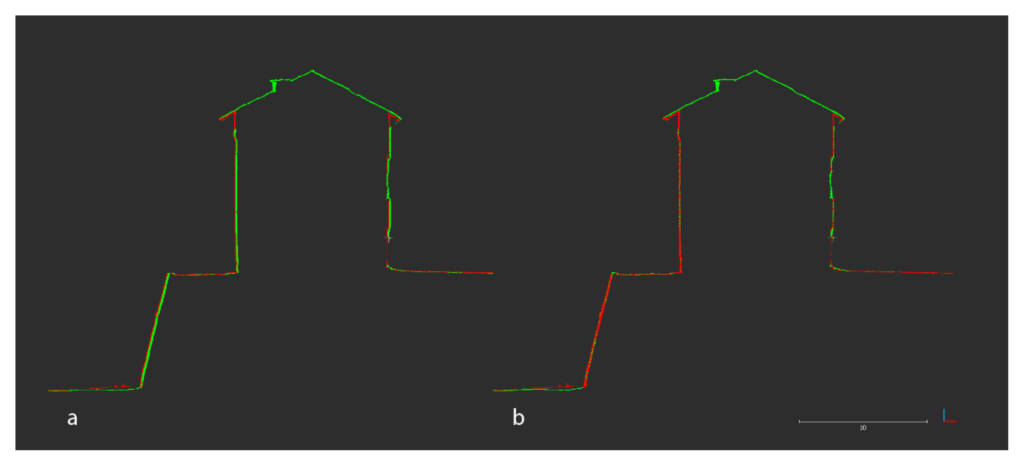
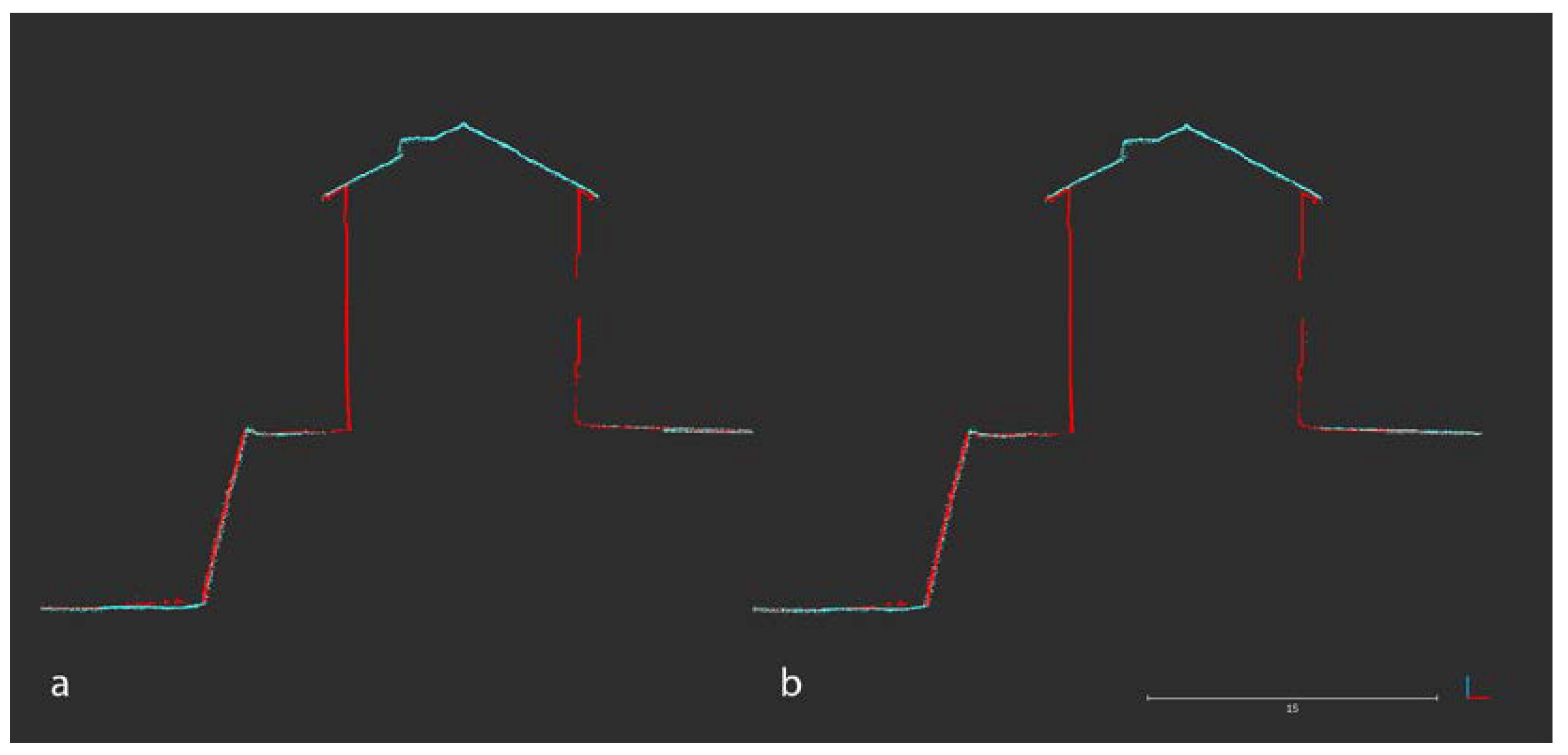
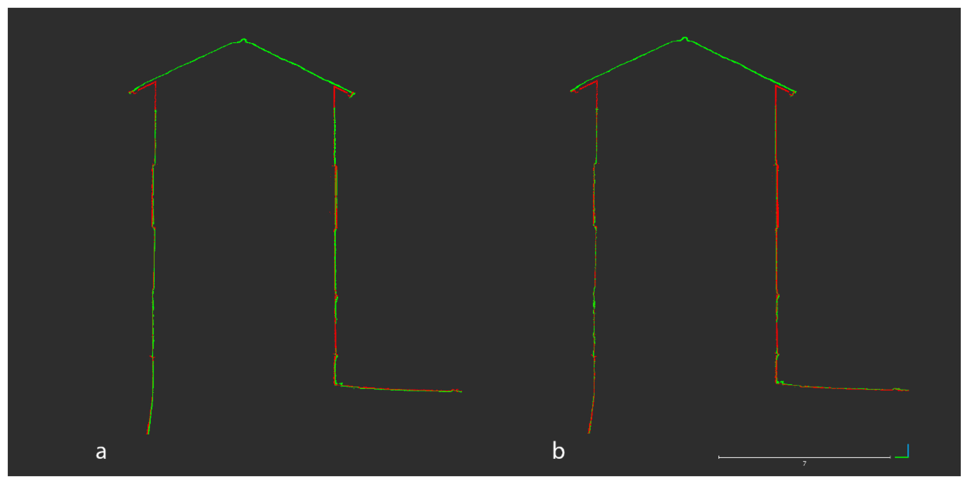
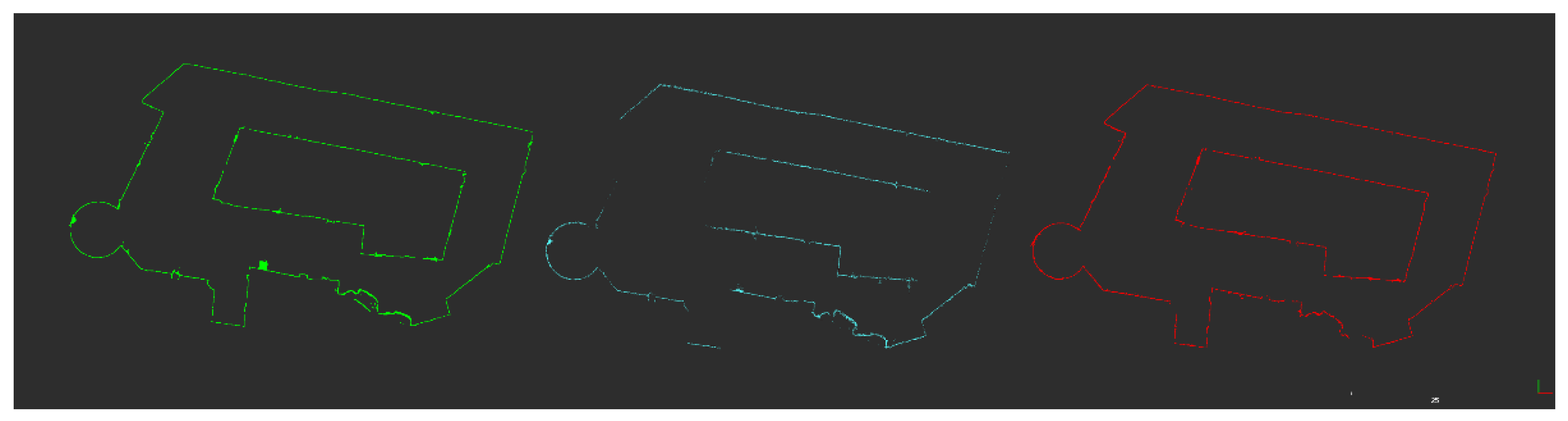
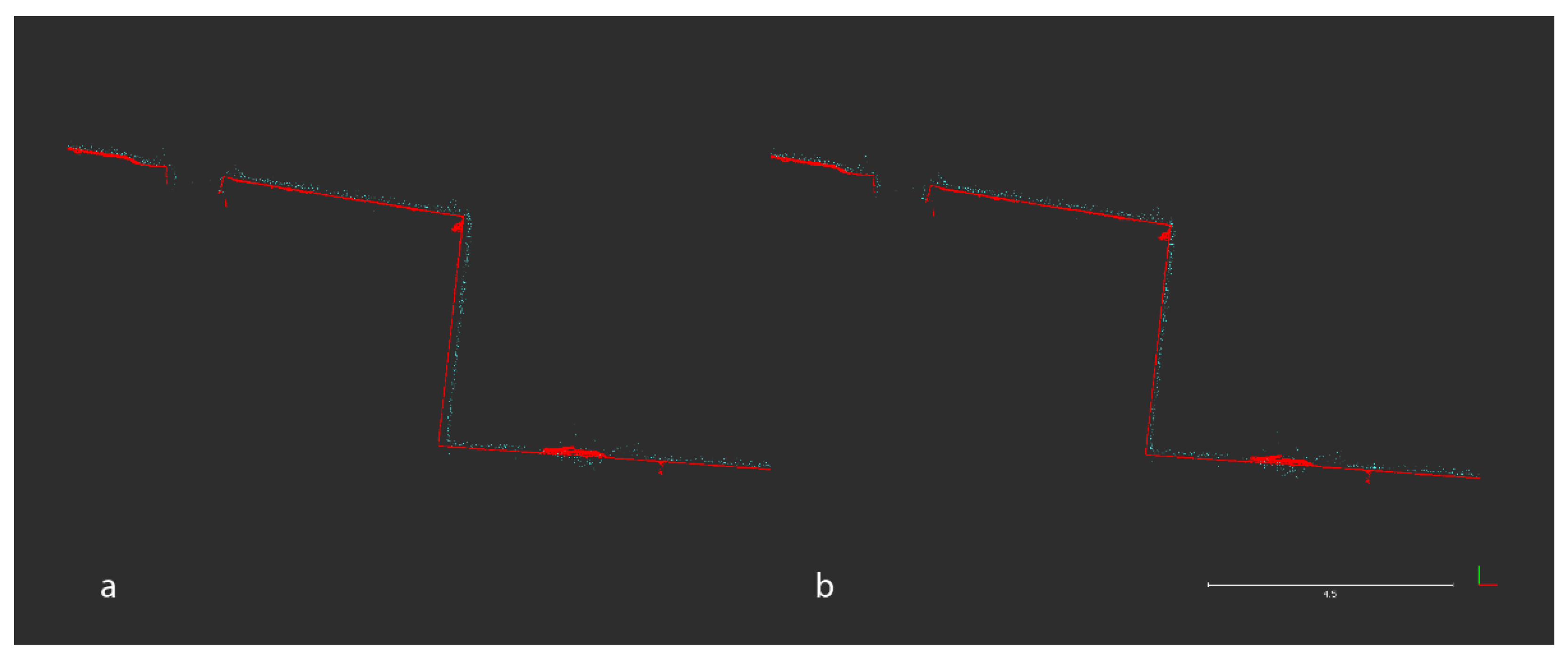
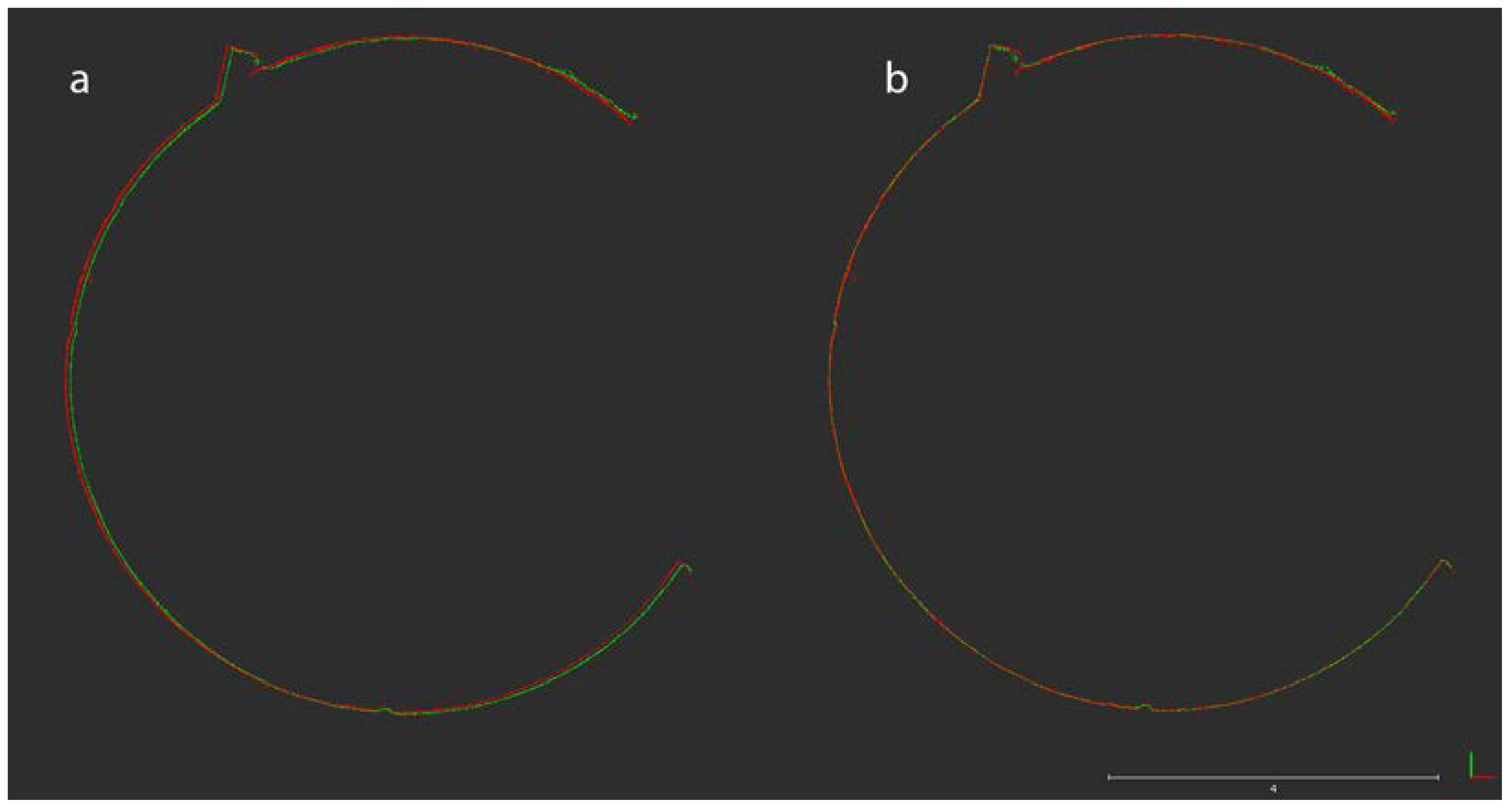
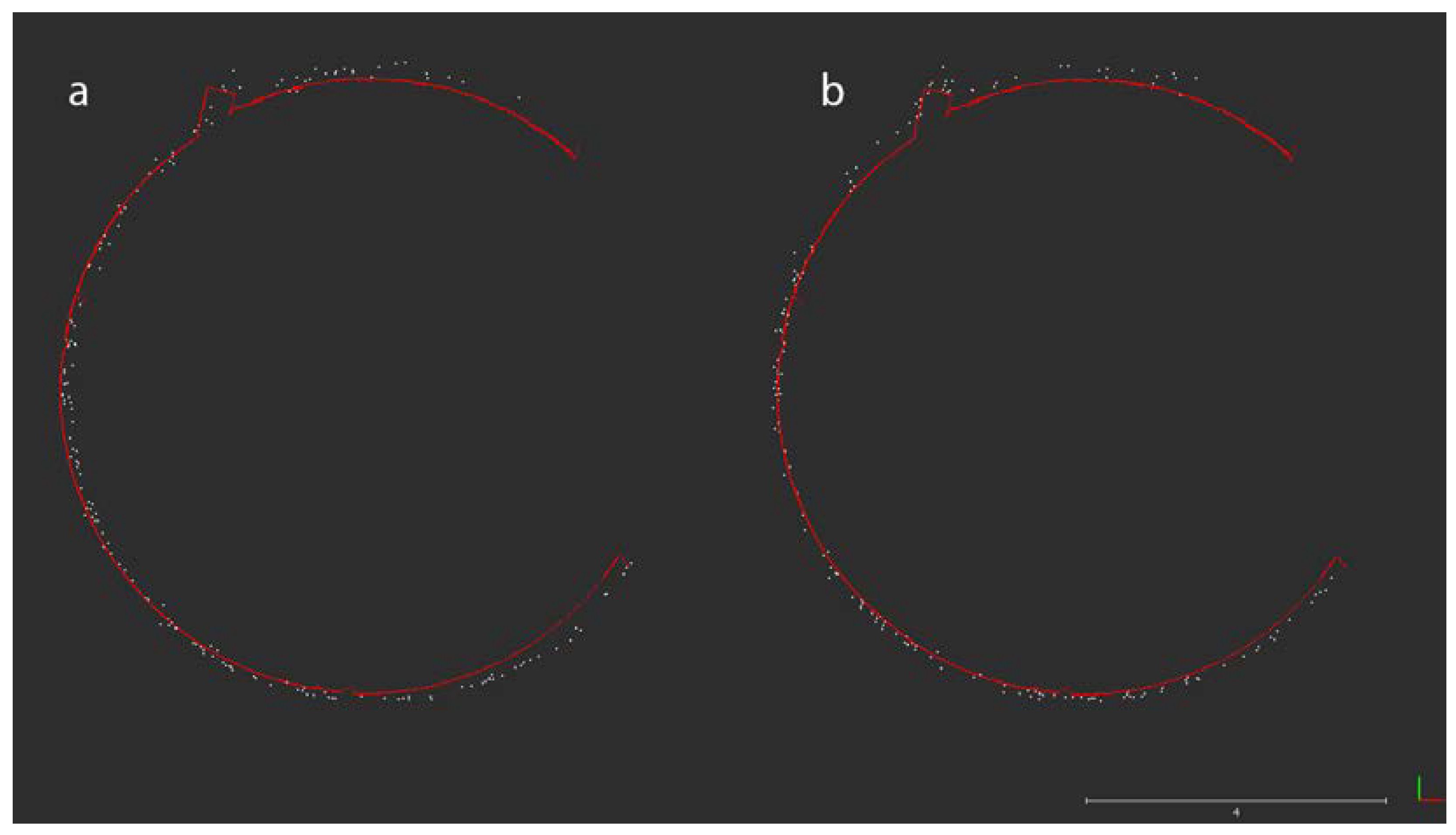
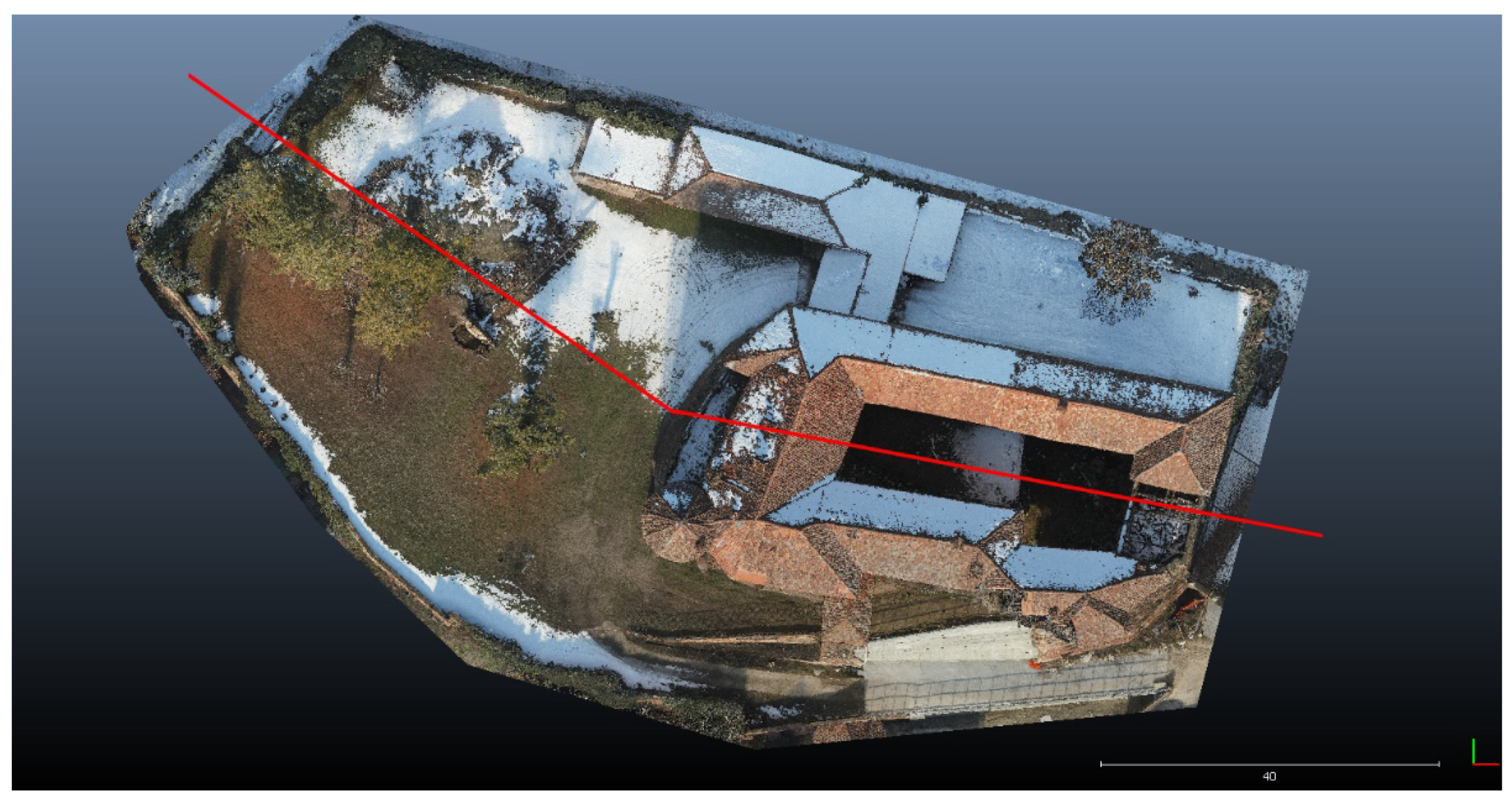
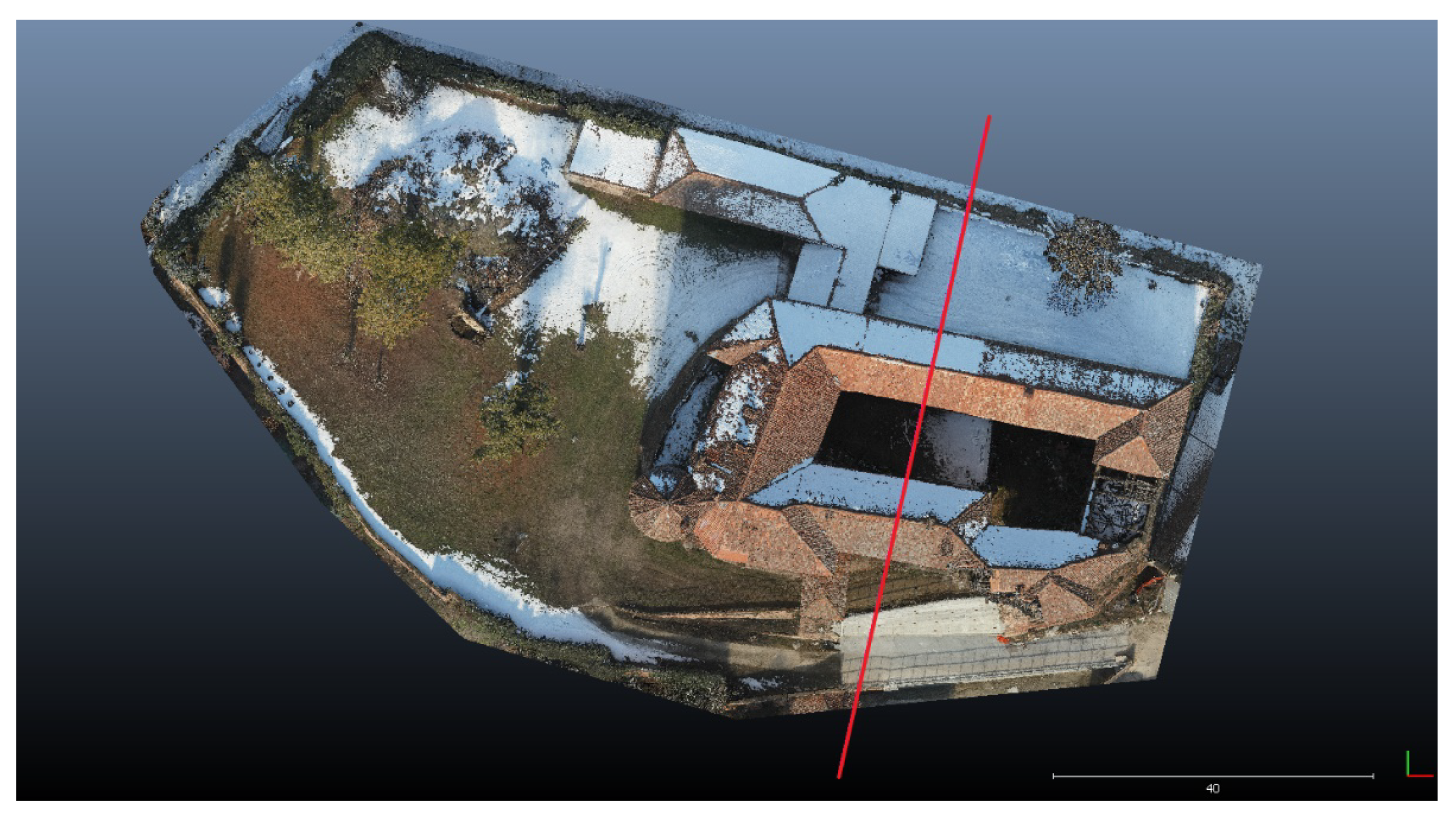
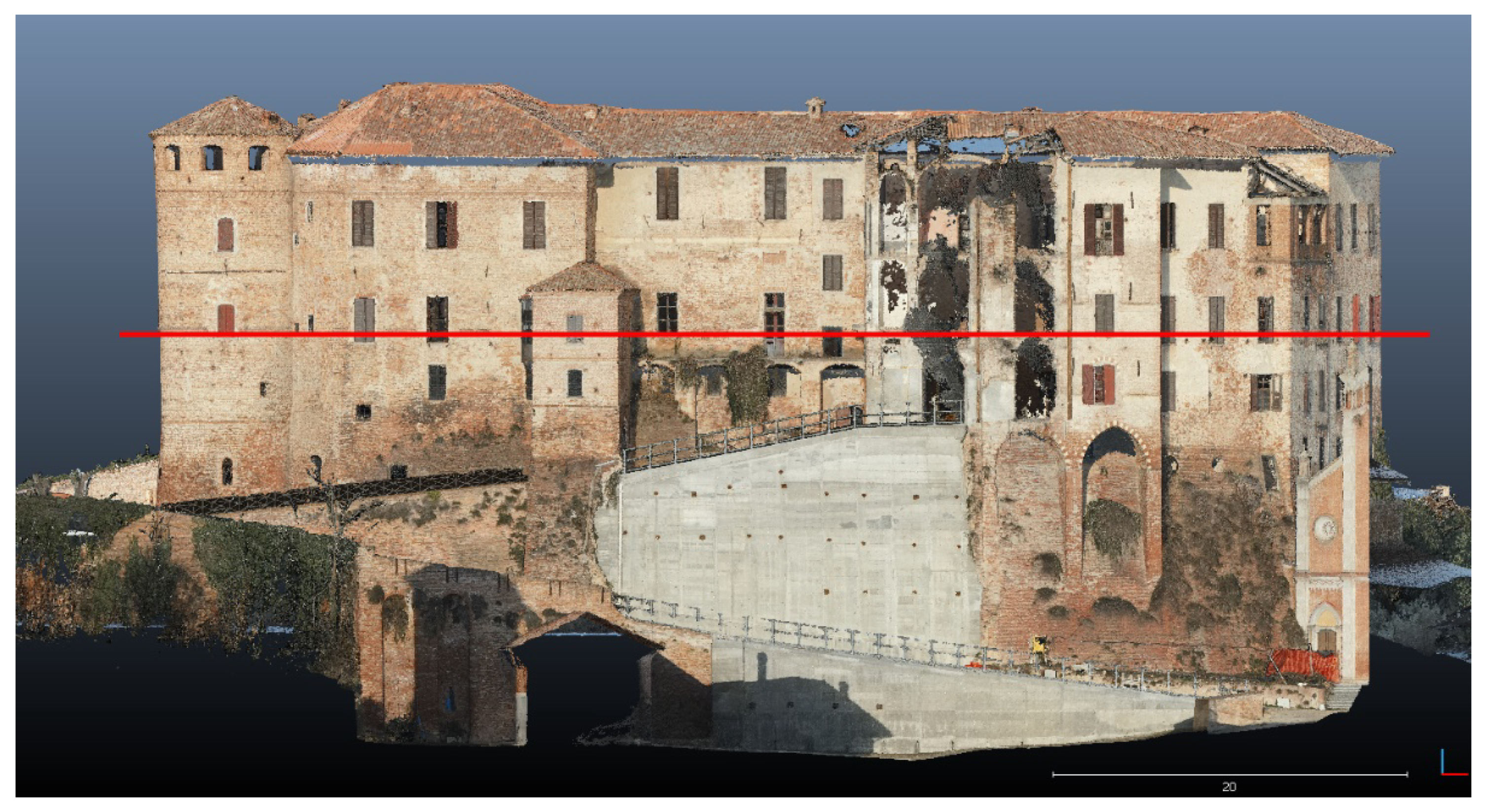
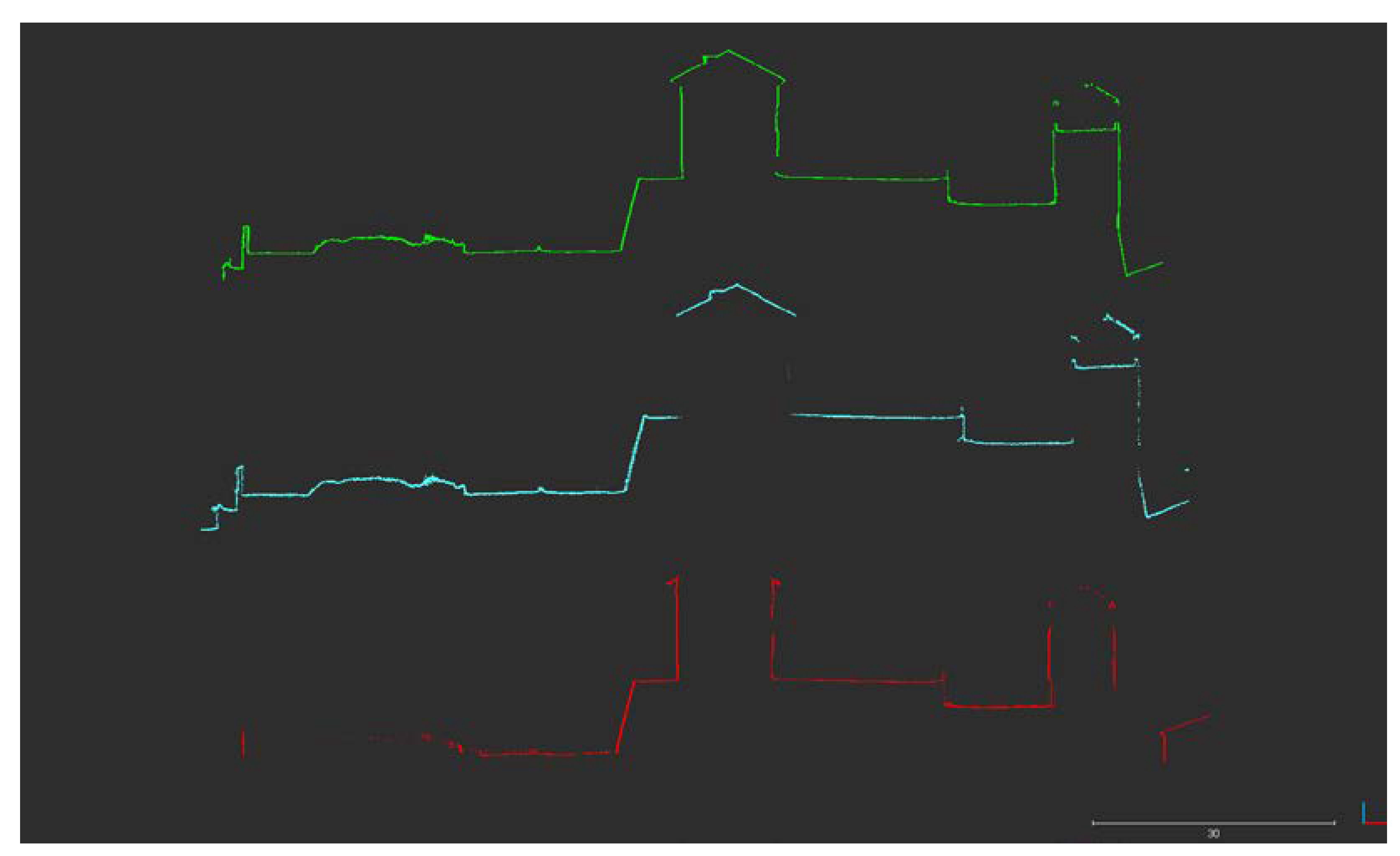
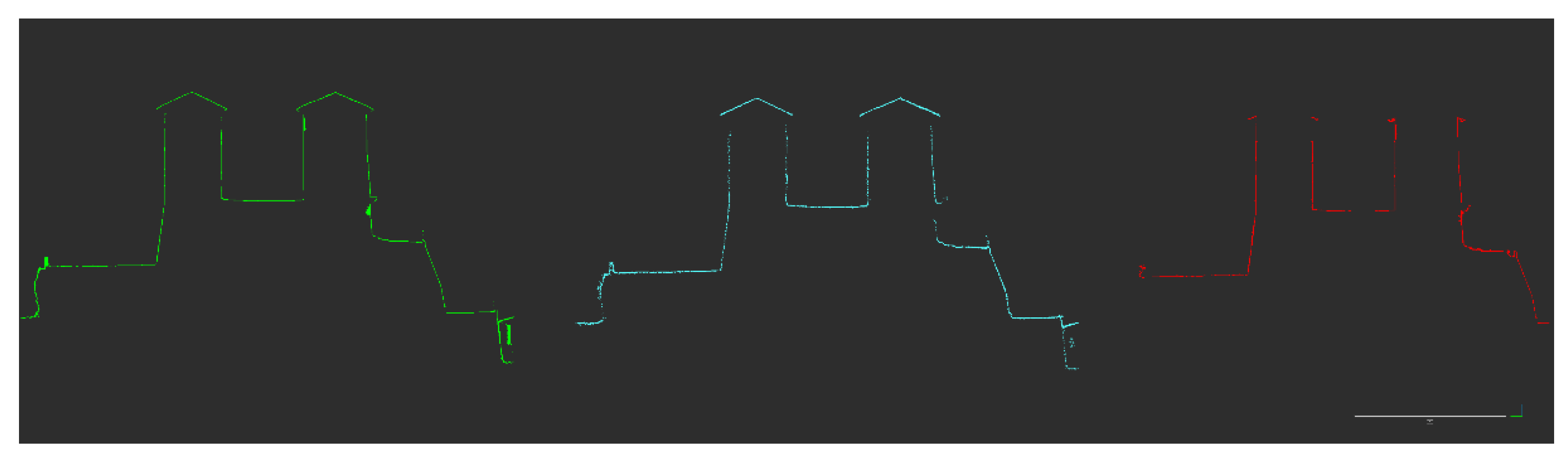
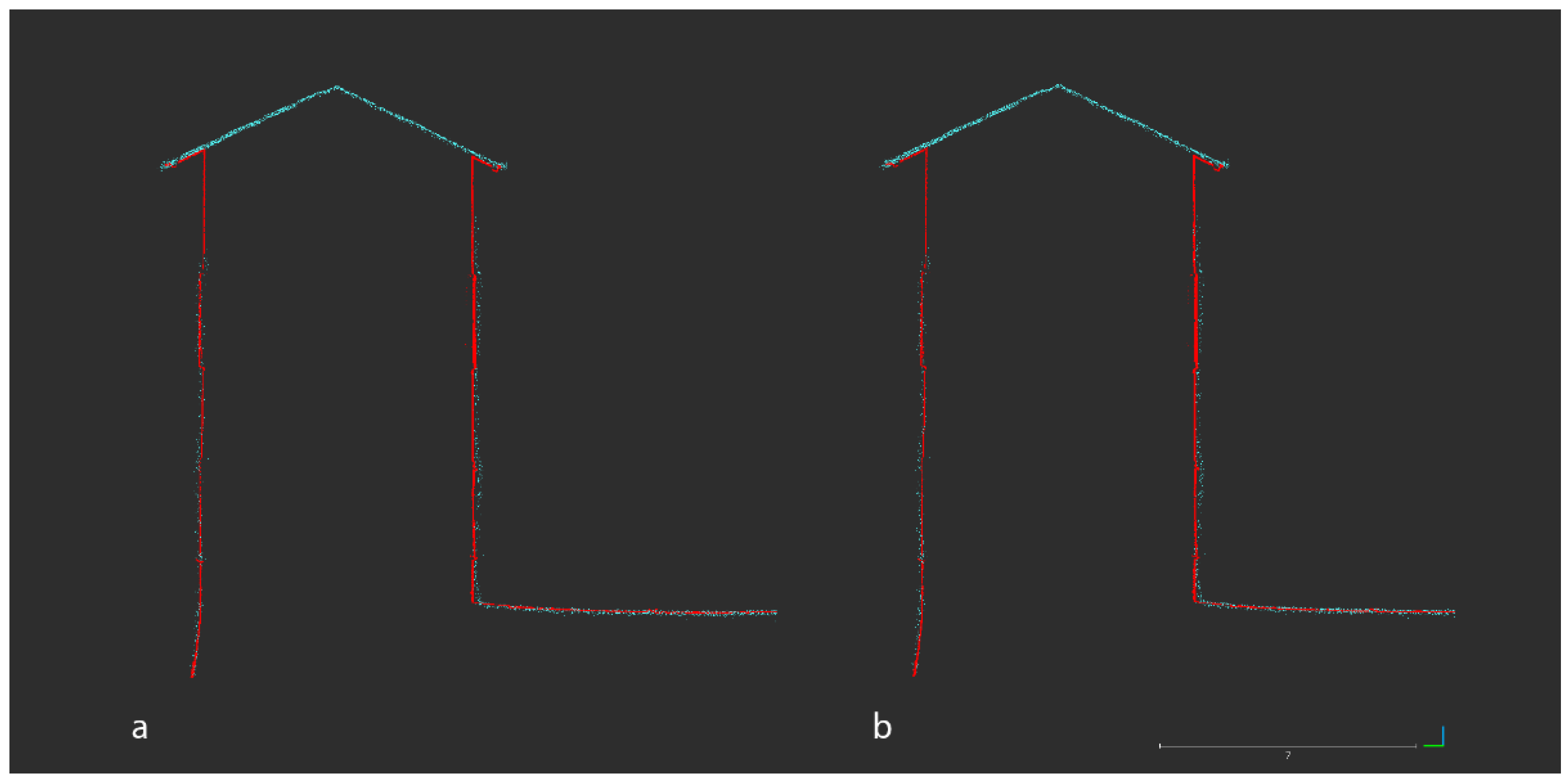
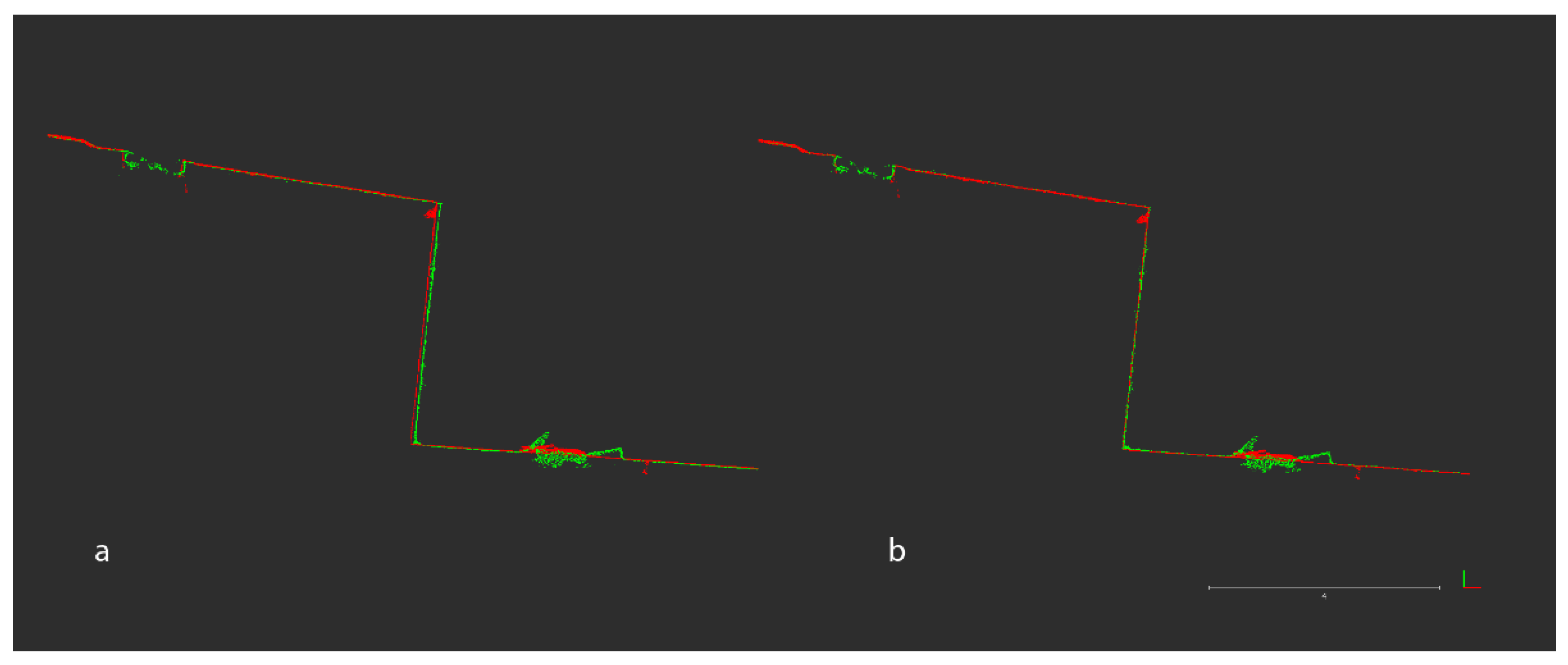
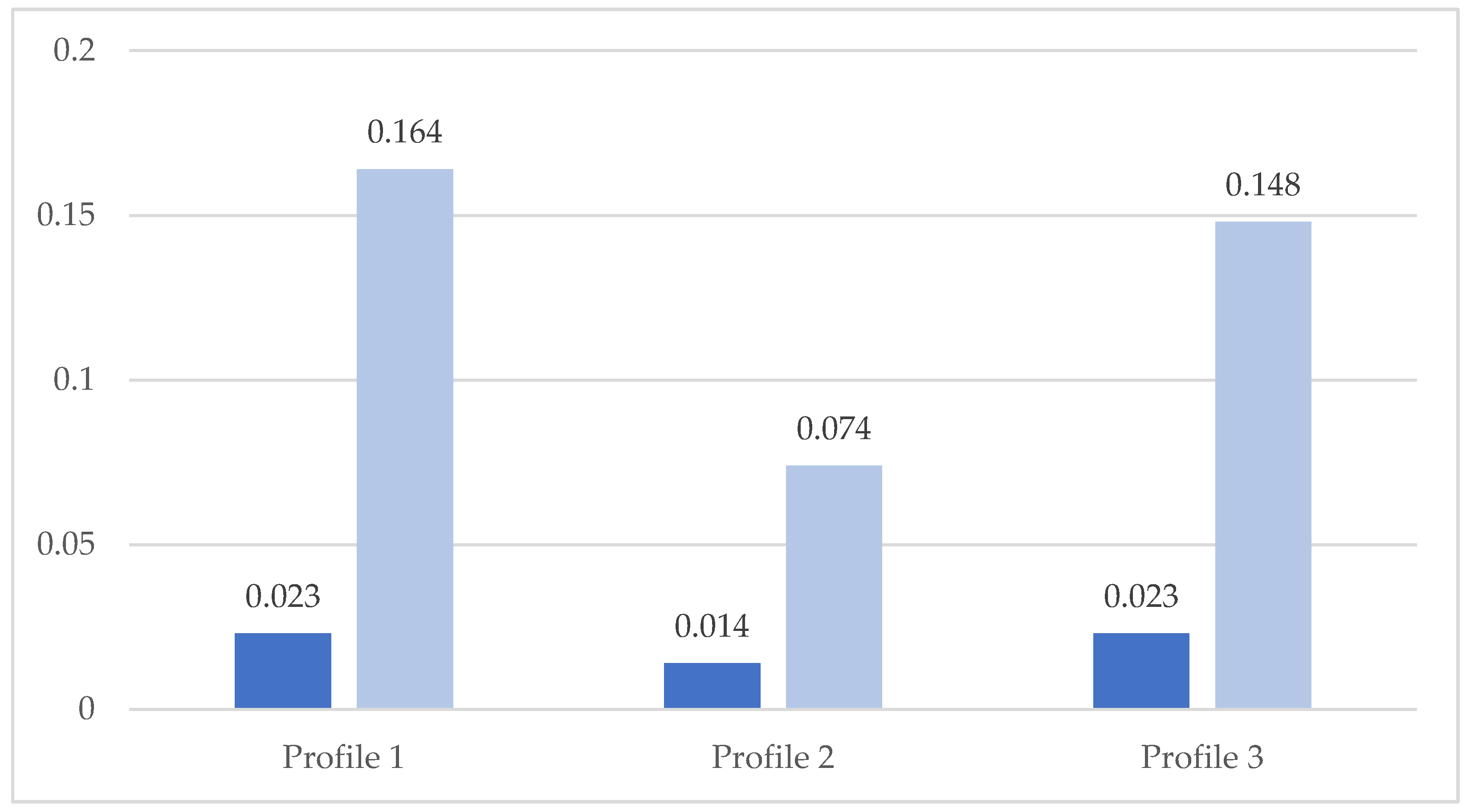
4.1.3. Profile Analyses
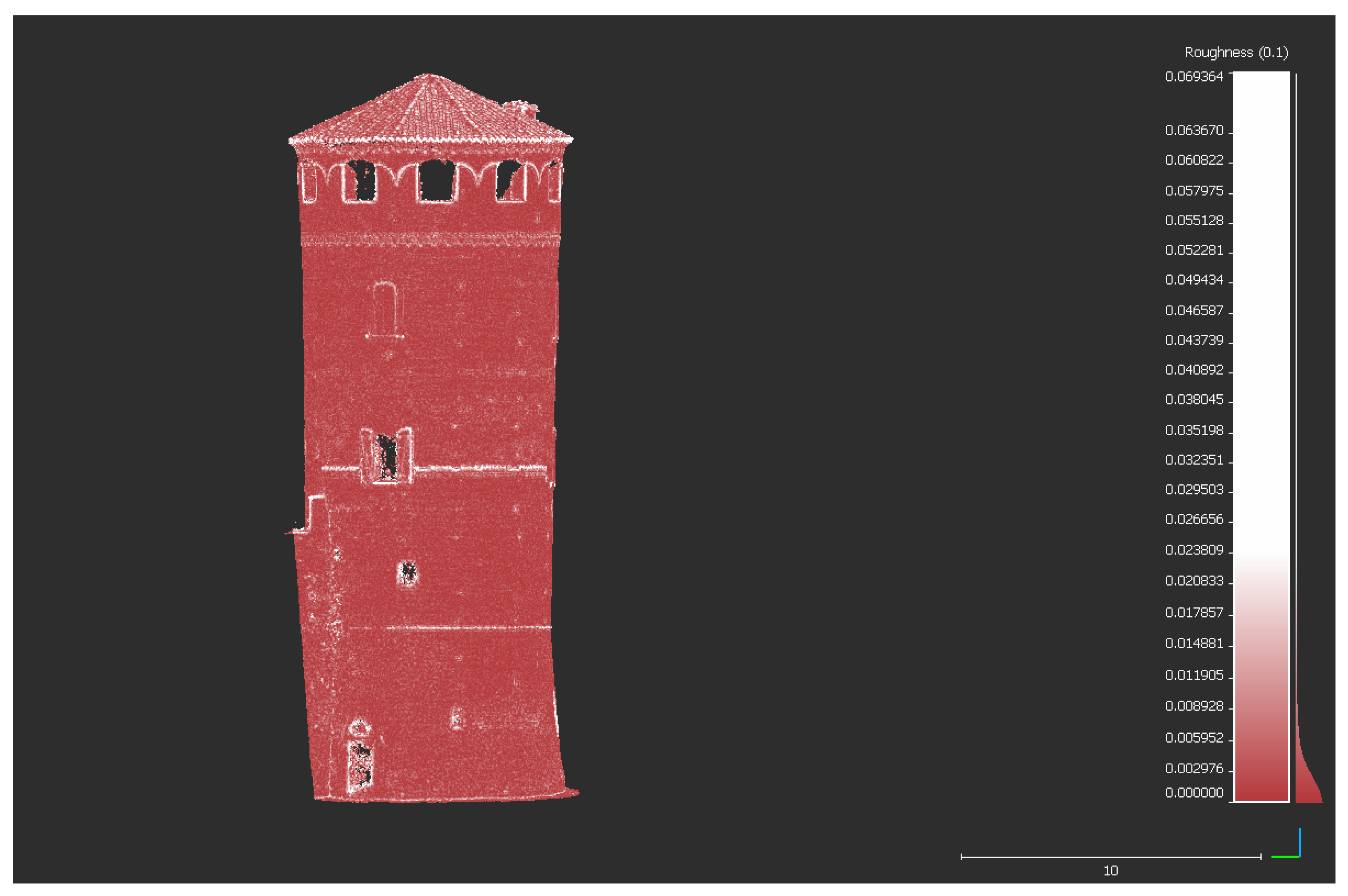
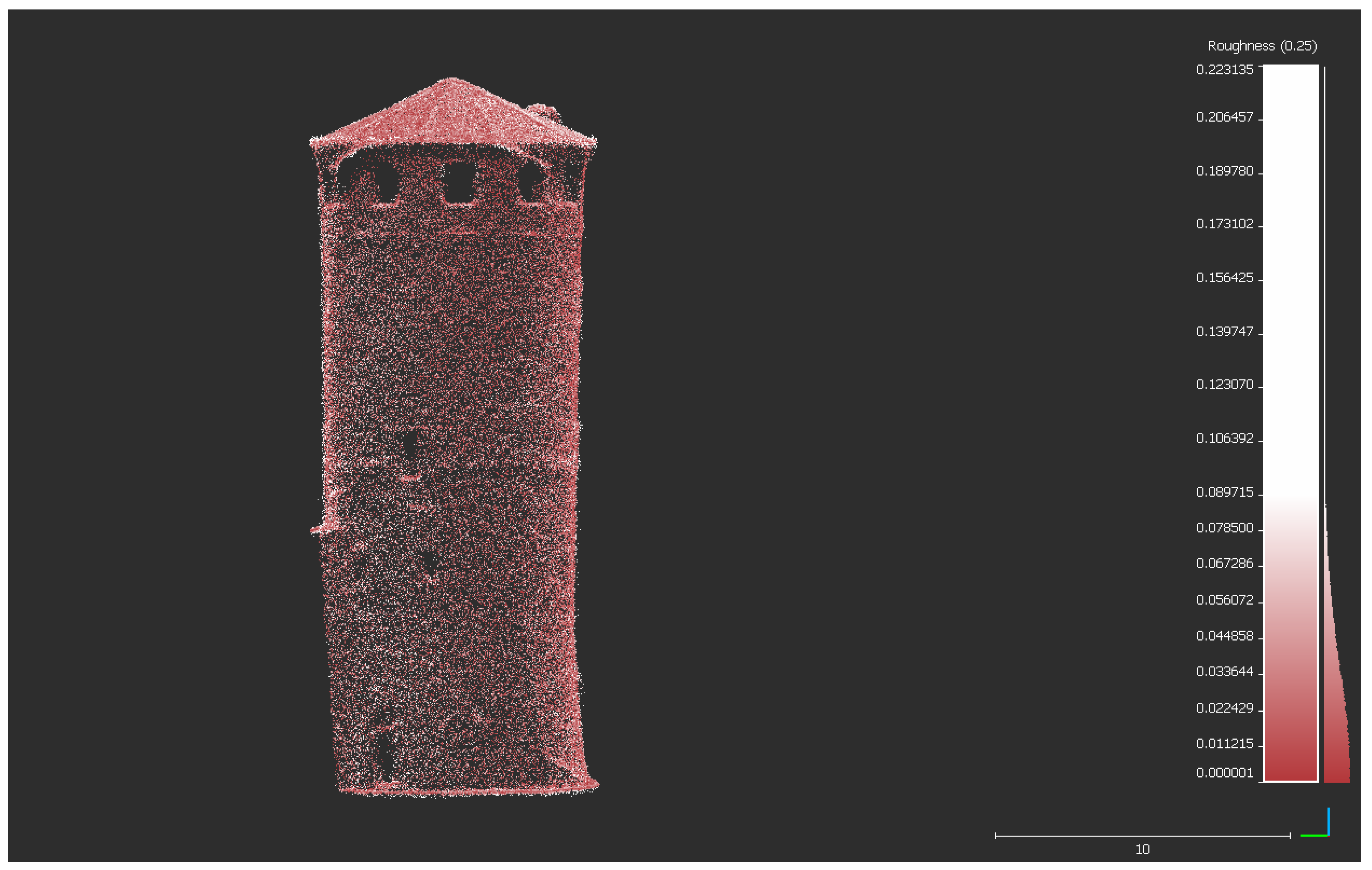
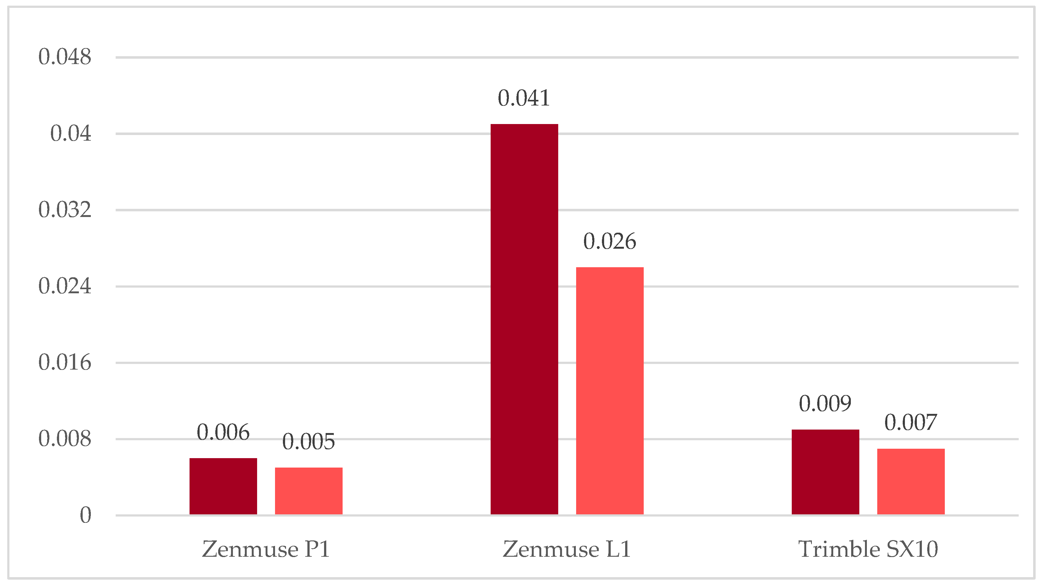
4.1.4. Roughness Analysis of the Tower
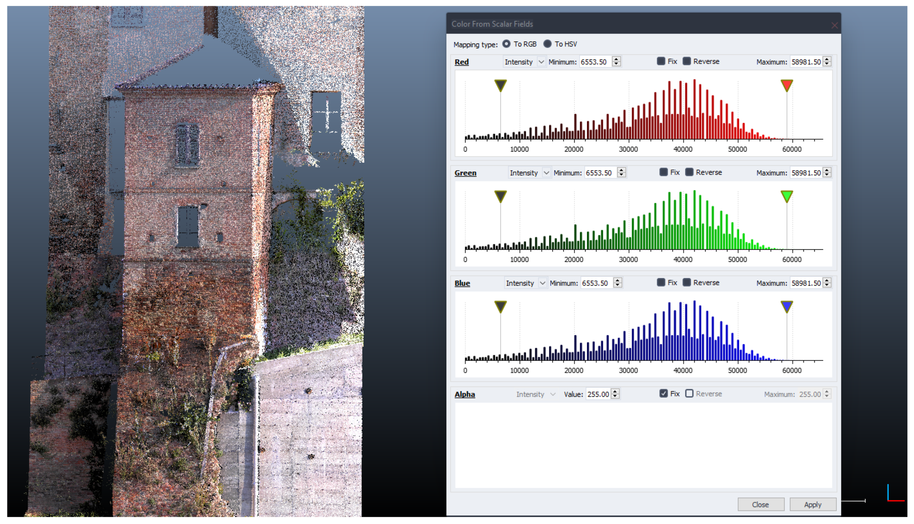
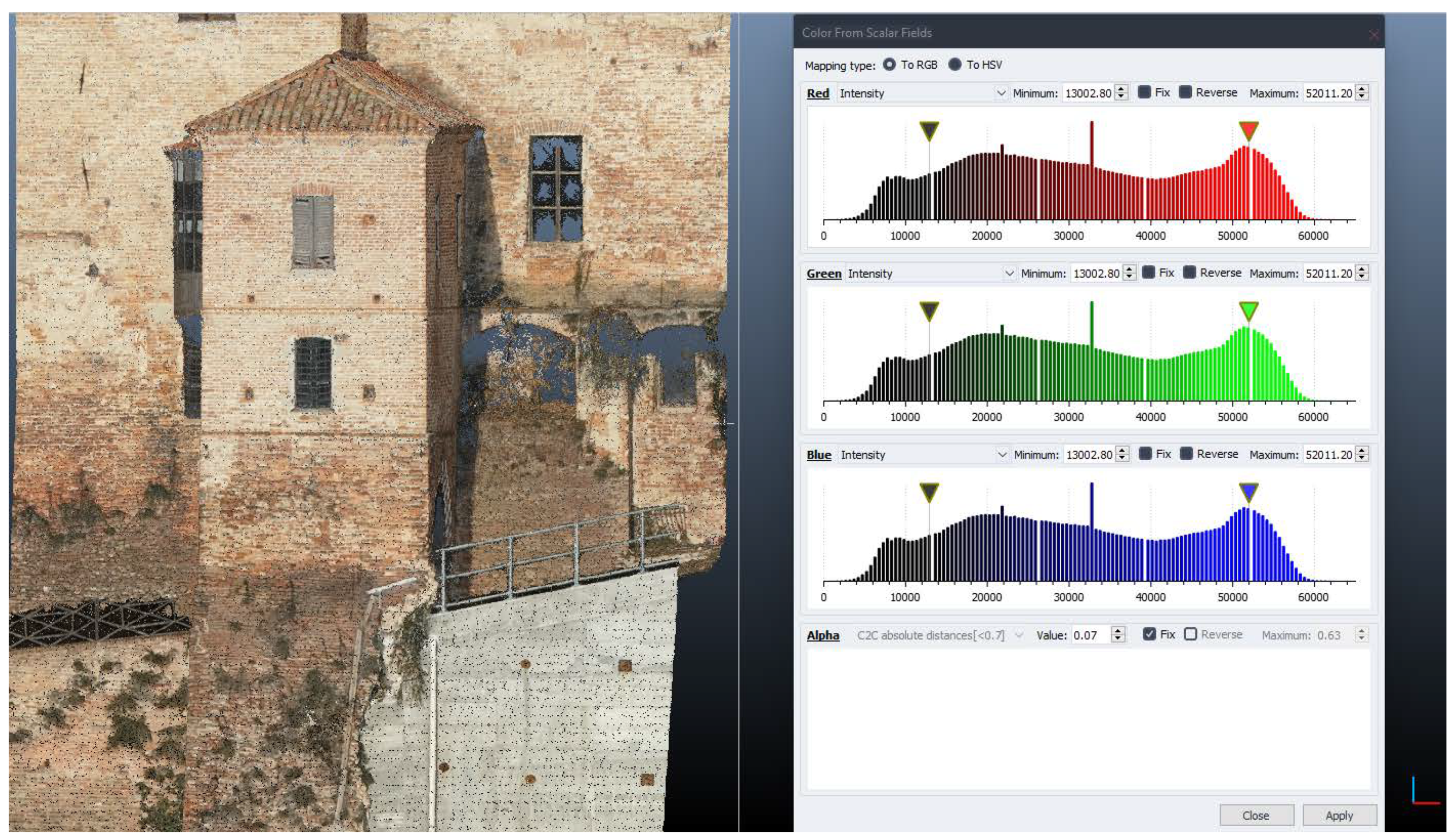
4.2. Radiometric Values Analysis
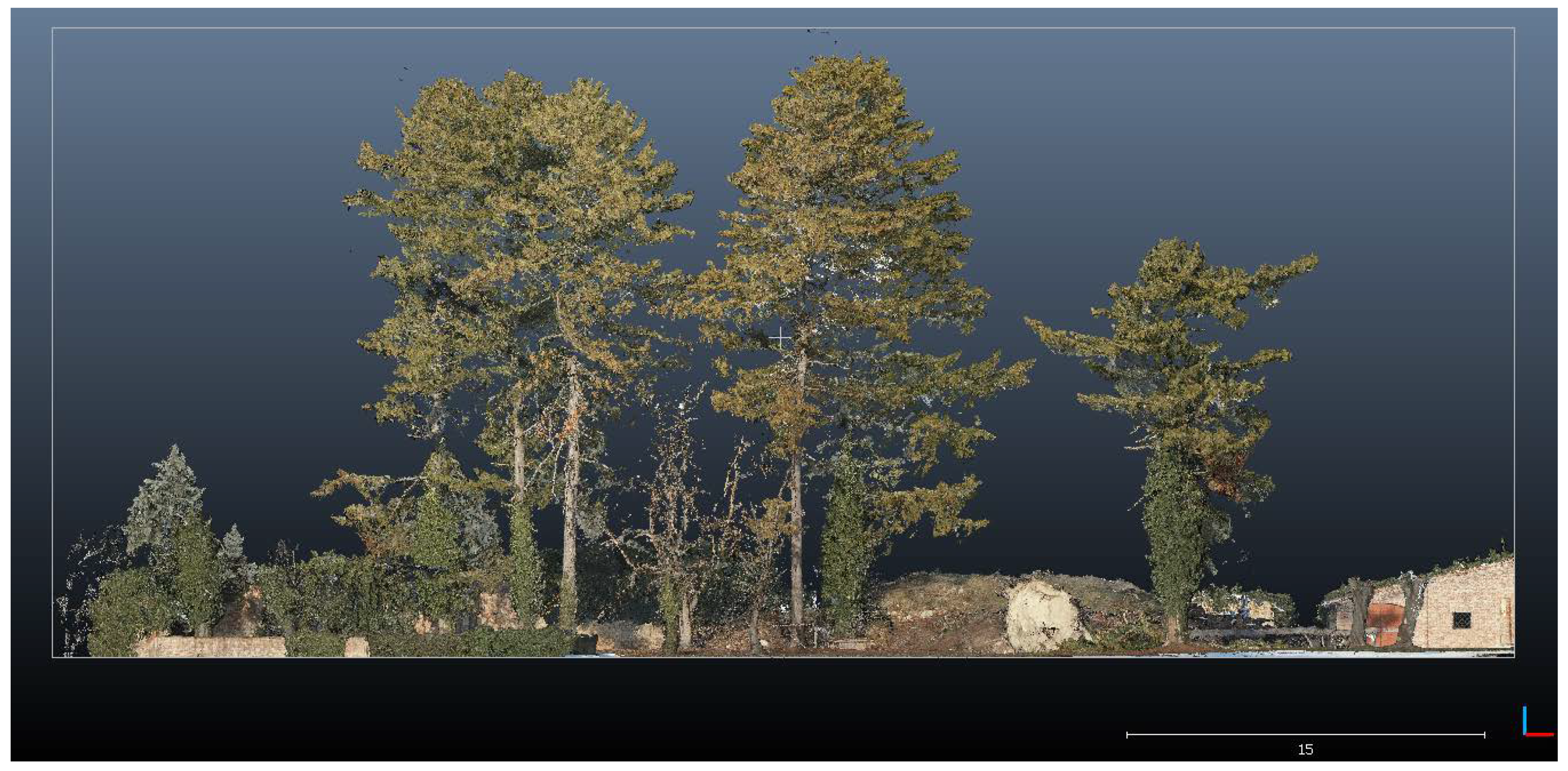
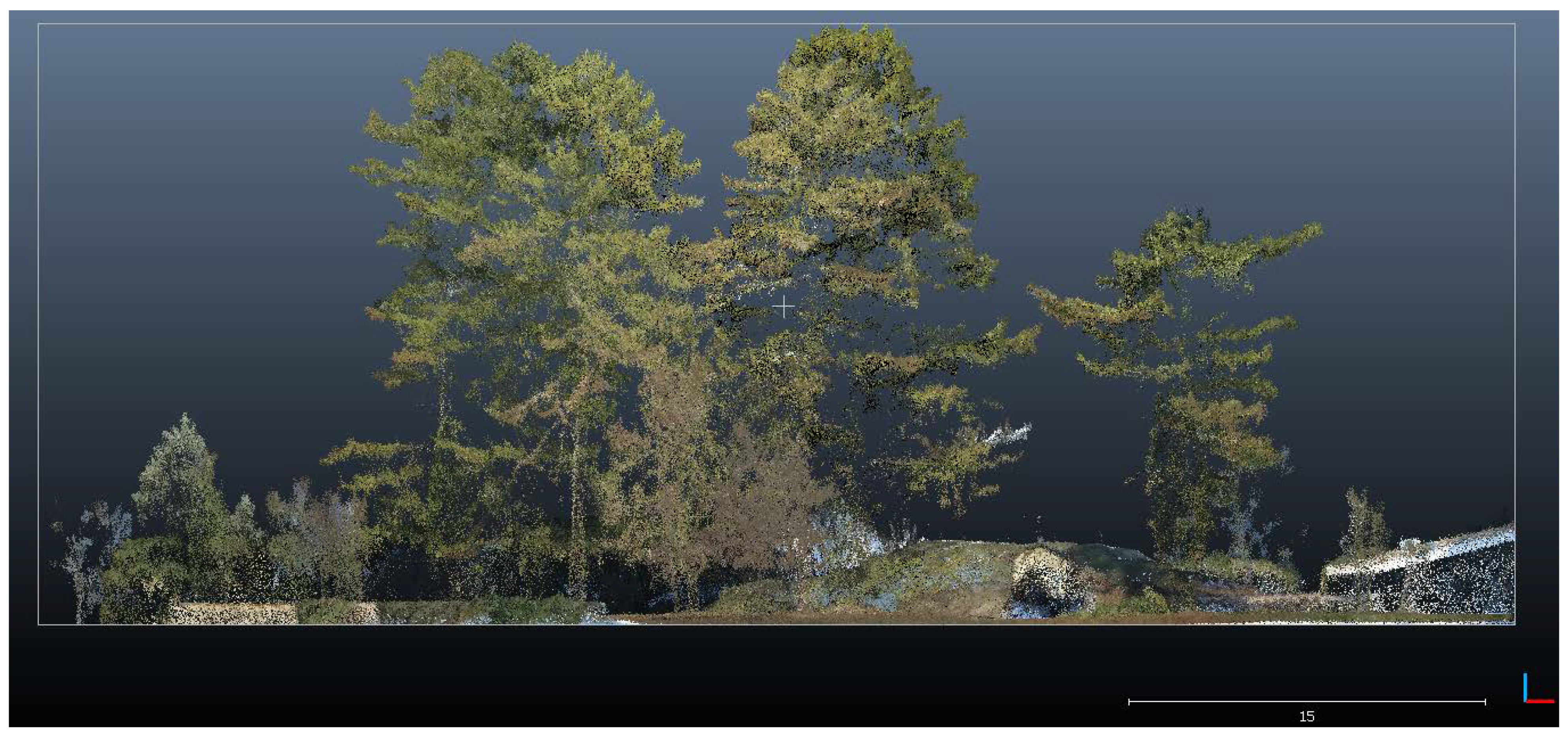
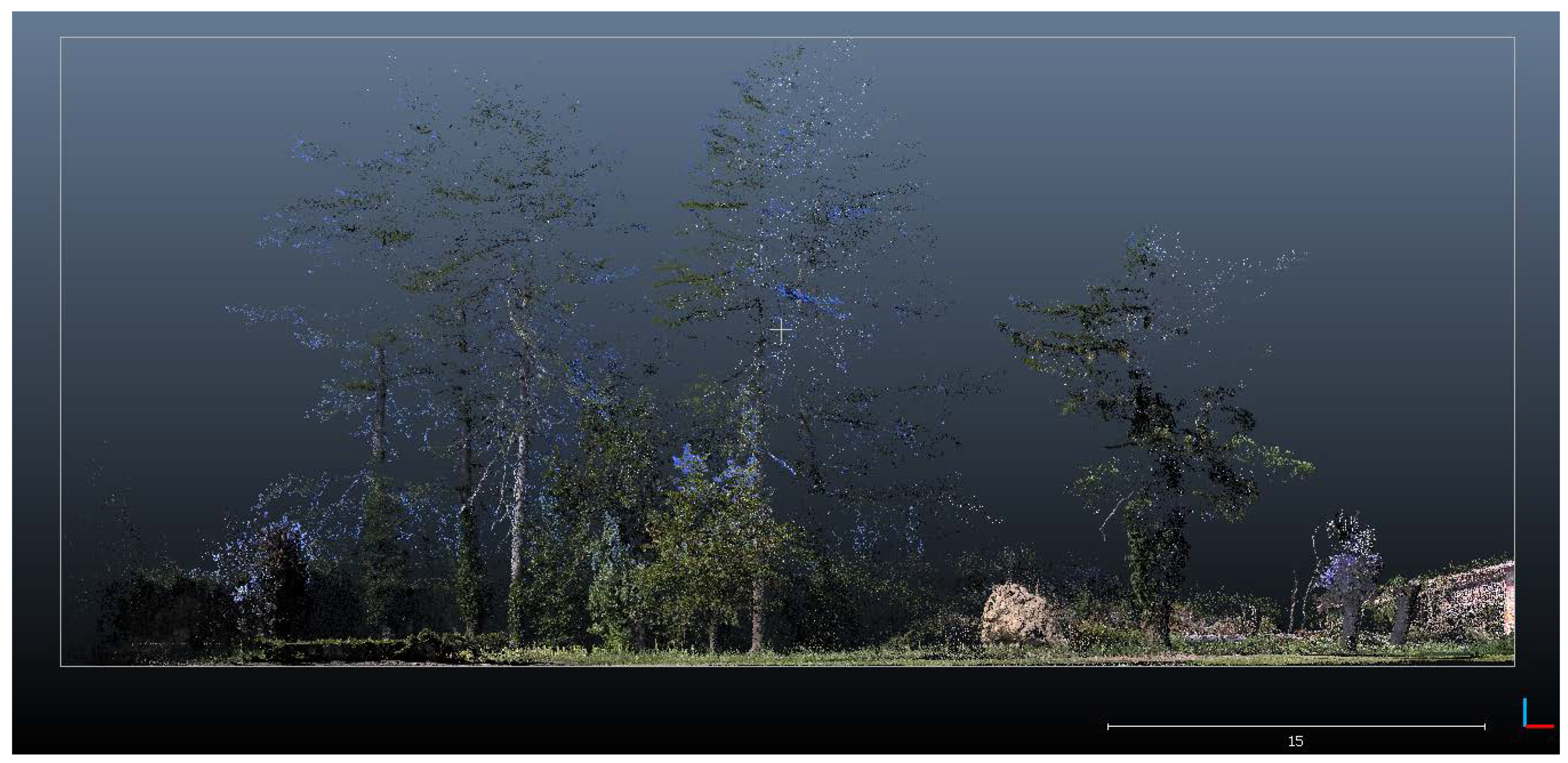
4.3. Vegetation Short Analysis
5. Results
6. Discussion
7. Conclusions
Author Contributions
Funding
Institutional Review Board Statement
Informed Consent Statement
Data Availability Statement
Acknowledgments
Conflicts of Interest
References
- DJI Website. Available online: https://www.dji.com (accessed on 21 June 2022).
- Trimble Website. Available online: https://www.trimble.com/en (accessed on 21 June 2022).
- Sani, N.H.; Tahar, K.N.; Maharjan, G.R.; Matos, J.C.; Muhammad, M. 3D reconstruction of building model using UAV point clouds. In Proceedings of the International Archives of the Photogrammetry, Remote Sensing and Spatial Information Sciences, Nice, France, 6–11 June 2022; Volume XLIII-B2-2022; pp. 455–460. [Google Scholar] [CrossRef]
- Cledat, E.; Skaloud, J. Fusion of photo with airborne laser scanning. ISPRS Ann. Photogramm. Remote Sens. Spatial Inf. Sci 2020, V-1-2020, 173–180. [Google Scholar] [CrossRef]
- Ekaso, D.; Nex, F.; Kerle, N. Accuracy assessment of real-time kinematics (RTK) measurements on unmanned aerial vehicles (UAV) for direct geo-referencing. Geo-Spat. Inf. Sci. 2020, 23, 165–181. [Google Scholar] [CrossRef] [Green Version]
- Štroner, M.; Urban, R.; Línková, L. A New Method for UAS Lidar Precision Testing Used for the Evaluation of an Affordable DJI Zenmuse L1 Scanner. Remote Sens. 2021, 13, 4811. [Google Scholar] [CrossRef]
- Gaspari, F.; Ioli, F.; Barbieri, F.; Belcore, E.; Pinto, L. Integration of UAS-LiDAR and UAS-photogrammetry for infrastructure monitoring and bridge assessment. In Proceedings of the International Archives of the Photogrammetry, Remote Sensing and Spatial Information Sciences, Nice, France, 6–11 June 2022; Volume XLIII-B2-2022, pp. 995–1002. [Google Scholar] [CrossRef]
- Nex, F.; Armenakis, C.; Cramer, M.; Cucci, D.A.; Gerke, M.; Honkavaara, E.; Skaloud, J. UAV in the advent of the twenties: Where we stand and what is next. ISPRS J. Photogramm. Remote Sens. 2020, 184, 215–242. [Google Scholar] [CrossRef]
- Teppati Losè, L.; Matrone, F.; Chiabrando, F.; Giulio Tonolo, F.; Lingua, A.; Maschio, P. New developments in lidar UAS surveys. Performance analyses and validation of the DJI Zenmuse L1. In Proceedings of the International Archives of the Photogrammetry, Remote Sensing and Spatial Information Sciences, Nice, France, 6–11 June 2022; Volume XLIII-B1-2022, pp. 415–422. [Google Scholar] [CrossRef]
- Kersten, T.; Wolf, J.; Lindstaedt, M. Investigations into the accuracy of the UAS system DJI Matrice 300 RTK with the sensors Zenmuse P1 and L1 in the Hamburg test field. In Proceedings of the International Archives of the Photogrammetry, Remote Sensing and Spatial Information Sciences, Nice, France, 6–11 June 2022; Volume XLIII-B1-2022, pp. 339–346. [Google Scholar] [CrossRef]
- Peppa, M.V.; Morelli, L.; Mills, J.P.; Penna, N.T.; Remondino, F. Handcrafted and learning-based tie point features—Comparison using the EuroSDR RPAS benchmark dataset. In Proceedings of the International Archives of the Photogrammetry, Remote Sensing and Spatial Information Sciences, Nice, France, 6–11 June 2022; Volume XLIII-B2-2022, pp. 1183–1190. [Google Scholar] [CrossRef]
- CloudCompare Software. Available online: https://www.danielgm.net/cc/ (accessed on 21 June 2022).
- Bordone, R. Andar per Castelli da Asti Tutt’intorno; Milvia: Torino, Italy, 1976; ISBN 2020010144721. [Google Scholar]
- Sorisio, R. Ricerche Storico-Giuridiche su Frinco. Master’s Thesis, University of Turin, Turin, Italy, 1979. [Google Scholar]
- Lachat, E.; Landes, T.; Grussenmeyer, P. Investigation of a Combined Surveying and Scanning Device: The Trimble SX10 Scanning Total Station. Sensors 2017, 17, 730. [Google Scholar] [CrossRef] [PubMed] [Green Version]
- Lachat, E.; Landes, T.; Grussenmeyer, P. First experiences with the Trimble SX10 scanning total station for building facade survey. In Proceedings of the International Archives of the Photogrammetry, Remote Sensing and Spatial Information Sciences, Nafplio, Greece, 1–3 March 2017; Volume XLII-2/W3, pp. 405–412. [Google Scholar] [CrossRef] [Green Version]
- HighPix Company. Available online: https://www.highpix.it (accessed on 21 June 2022).
- Agisoft Metashape. Available online: https://www.agisoft.com (accessed on 21 June 2022).
- Ramalho de Oliveira, L.F.; Lassiter, H.A.; Wilkinson, B.; Whitley, T.; Ifju, P.; Logan, S.R.; Peter, G.F.; Vogel, J.G.; Martin, T.A. Moving to Automated Tree Inventory: Comparison of UAS-Derived Lidar and Photogrammetric Data with Manual Ground Estimates. Remote Sens. 2021, 13, 72. [Google Scholar] [CrossRef]
- Jaakkola, A.; Hyyppä, J.; Kukko, A.; Yu, X.; Kaartinen, H.; Lehtomäki, M.; Lin, Y. A low-cost multi-sensoral mobile mapping system and its feasibility for tree measurements. ISPRS J. Photogramm. Remote Sens. 2010, 65, 514–522. [Google Scholar] [CrossRef]
- Zhang, F.; Hassanzadeh, A.; Kikkert, J.; Pethybridge, S.J.; Van Aardt, J. Comparison of UAS-Based Structure-from-Motion and LiDAR for Structural Characterization of Short Broadacre Crops. Remote Sens. 2021, 13, 3975. [Google Scholar] [CrossRef]
- Mugnai, F.; Masiero, A. Integrating UAS Photogrammetry and Digital Image Correlation for High-Resolution Monitoring of Large Landslides. Preprints 2022, 2022010248. [Google Scholar] [CrossRef]
- Pinto, L.; Bianchini, F.; Nova, V.; Passoni, D. Low-Cost UAS Photogrammetry for road Infrastructures’inspection. In Proceedings of the International Archives of the Photogrammetry, Remote Sensing and Spatial Information Sciences, Nice, France, 14–21 June 2020; Volume XLIII-B2-2020, pp. 1145–1150. [Google Scholar] [CrossRef]
- Yordanov, V.; Biagi, L.; Truong, X.Q.; Brovelli, M.A. Landslide surveys using low-cost UAV and FOSS photogrammetric workflow. In Proceedings of the International Archives of the Photogrammetry, Remote Sensing and Spatial Information Sciences, Nice, France, 6–11 June 2022; Volume XLIII-B2-2022; pp. 493–499. [Google Scholar] [CrossRef]


| Detection Range | Point Rate | Ranging Accuracy (RMS 1σ) | Field of View (Non-Repetitive) | Field of View (Repetitive) |
|---|---|---|---|---|
| 450 m~80% reflectivity, 0 klx; | Single return: max 240,000 pts/s | 3 cm~100 m | 70.4° (horizontal) | 70.4° (horizontal) |
| 190 m~10% reflectivity, 100 klx | Multiple return: max 480,000 pts/s | 77.2° (vertical) | 4.5° (vertical) |
| Pixel Size | Pixels | Sensor Size | Aperture Range | Photo Size |
|---|---|---|---|---|
| 4.4 μm | 45 megapixels | 35.9 × 24 mm (Full Frame) | f/2.8–f/16 | 3:2 (8192 × 5460) |
| Sensor | Total Images | Tie Points (High Accuracy) | Dense Cloud (High Quality) | 3D Model (Medium Quality) |
|---|---|---|---|---|
| DJI Zenmuse P1 | 477 (336 oblique/141 nadiral) | 304,997 pts | 349,218,444 pts | 4,341,817 faces |
| Coordinate System | East Accuracy (m) | Nord Accuracy (m) | Altitude Accuracy (m) | Accuracy (°) |
|---|---|---|---|---|
| WGS 84/UTM Zone 32N + EGM2008 | 0.012 | 0.015 | 0.05 | 10.00 |
| Zenmuse L1 (pts) | Zenmuse P1 (pts) | Trimble SX10 (pts) |
|---|---|---|
| 75,251 | 1,255,812 | 2,571,443 |
| C2C | Max Distance (m) | Standard Deviation (m) | Mean Distance (m) |
|---|---|---|---|
| L1 > SX10 | 0.3 | 0.089 | 0.076 |
| P1 > SX10 | 0.1 | 0.119 | 0.044 |
| L1 > P1 | 0.1 | 0.061 | 0.054 |
| Range (m) | Point Coverage |
|---|---|
| 0.00–0.04 | 34% |
| 0.04–0.08 | 28% |
| 0.08–0.12 | 22% |
| 0.12–0.30 | 16% |
| Range (m) | Point Coverage |
|---|---|
| 0.00–0.02 | 35% |
| 0.02–0.04 | 30% |
| 0.04–0.08 | 31% |
| 0.08–0.10 | 3% |
| Range (m) | Point Coverage |
|---|---|
| 0.00–0.02 | 33% |
| 0.02–0.04 | 26% |
| 0.04–0.08 | 28% |
| 0.08–0.10 | 13% |
| ICP | RMSe (m) | Shift on X | Shift on Y | Shift on Z |
|---|---|---|---|---|
| P1 > TLS | 0.05 | −0.057 | 0.018 | 0.006 |
| L1 > TLS | 0.19 | −0.101 | 0.036 | −0.199 |
| Zenmuse L1 (pts) | Zenmuse P1 (pts) | Trimble SX10 (pts) | |
|---|---|---|---|
| Profile 1 | 32,583 | 162,203 | 468,383 |
| Profile 2 | 14,168 | 91,889 | 159,803 |
| Profile 3 | 15,432 | 302,760 | 667,492 |
| RMSe (m) | Shift on X | Shift on Y | Shift on Z | |
|---|---|---|---|---|
| P1 aligned to TLS | 0.023 | −0.061 | 0.015 | 0.021 |
| L1 aligned to TLS | 0.164 | −0.011 | 0.003 | 0.042 |
| RMSe (m) | Shift on X | Shift on Y | Shift on Z | |
|---|---|---|---|---|
| P1 aligned to TLS | 0.014 | 0.000 | 0.023 | 0.030 |
| L1 aligned to TLS | 0.074 | 0.011 | 0.034 | 0.019 |
| RMSe (m) | Shift on X | Shift on Y | Shift on Z | |
|---|---|---|---|---|
| P1 aligned to TLS | 0.023 | −0.057 | 0.024 | 0.001 |
| L1 aligned to TLS | 0.148 | −0.071 | 0.029 | −0.009 |
| Data | Point Count | Local Neighbourhood Radius (m) | Standard Deviation (m) | RMSe (m) |
|---|---|---|---|---|
| Zenmuse L1 | 129,024 | 0.25 | 0.025 | 0.047 |
| Zenmuse P1 | 1,513,162 | 0.10 | 0.005 | 0.007 |
| Trimble SX10 | 2,571,443 | 0.10 | 0.007 | 0.009 |
Publisher’s Note: MDPI stays neutral with regard to jurisdictional claims in published maps and institutional affiliations. |
© 2022 by the authors. Licensee MDPI, Basel, Switzerland. This article is an open access article distributed under the terms and conditions of the Creative Commons Attribution (CC BY) license (https://creativecommons.org/licenses/by/4.0/).
Share and Cite
Diara, F.; Roggero, M. Quality Assessment of DJI Zenmuse L1 and P1 LiDAR and Photogrammetric Systems: Metric and Statistics Analysis with the Integration of Trimble SX10 Data. Geomatics 2022, 2, 254-281. https://doi.org/10.3390/geomatics2030015
Diara F, Roggero M. Quality Assessment of DJI Zenmuse L1 and P1 LiDAR and Photogrammetric Systems: Metric and Statistics Analysis with the Integration of Trimble SX10 Data. Geomatics. 2022; 2(3):254-281. https://doi.org/10.3390/geomatics2030015
Chicago/Turabian StyleDiara, Filippo, and Marco Roggero. 2022. "Quality Assessment of DJI Zenmuse L1 and P1 LiDAR and Photogrammetric Systems: Metric and Statistics Analysis with the Integration of Trimble SX10 Data" Geomatics 2, no. 3: 254-281. https://doi.org/10.3390/geomatics2030015
APA StyleDiara, F., & Roggero, M. (2022). Quality Assessment of DJI Zenmuse L1 and P1 LiDAR and Photogrammetric Systems: Metric and Statistics Analysis with the Integration of Trimble SX10 Data. Geomatics, 2(3), 254-281. https://doi.org/10.3390/geomatics2030015