Effects of Training Parameter Concept and Sample Size in Possibilistic c-Means Classifier for Pigeon Pea Specific Crop Mapping

Abstract

This research work aims to study the effect of training parameter concept and sample size in the process of classification by using a fuzzy Possibilistic c-Means (PCM) approach for Pigeon Pea specific crop mapping. For specific class extraction, the “mean” of the training data is considered as a training parameter of the classification algorithm. In this study, we proposed an “Individual Sample as Mean” (ISM) approach where the individual training sample is accounted as a mean parameter for the fuzzy PCM classifier. In order to avoid the spectral overlap of target Pigeon pea crop with other crops in the study area, a temporal indices database was generated from Sentinel 2A/2B satellite images acquired during the 2019–2020 Pigeon Pea crop cycle. The spectral dimensionality of temporal data was reduced to extract the required bands to achieve maximum enhancement of the target crop class in the temporal data. Further, the training sample size was increased to study the heterogeneity within the class in the classified output. The proposed ISM approach delivered a higher mean membership difference (MMD) between the Pigeon Pea crop and the co-cultivated Cotton crop as compared to the conventional mean method. This indicated that a better separation was achieved between the target crop and the spectrally similar crop grown, that were cultivated in the same study area. When the sample size was gradually increased from 5 to 60, the MMD values within the Pigeon Pea test fields remained in the range 0.013–0.02, thereby implying that the proposed algorithm works better even with a small number of training samples. The heterogeneity was better handled using the proposed ISM approach since the variance obtained within Pigeon Pea field was only 0.008, as compared to that of 0.02 achieved using the conventional mean approach.

1. Introduction

India is the primary centre of the origin and diversification for the Pigeon Pea crop. India is also the largest producer (over 85%) and consumer of the Pigeon pea crop with an annual production of 4.2 million metric tonnes in the year 2017 [1]. This crop is grown in regions with temperatures ranging from 26 °C to 30 °C in the monsoon season (June to October) and 17 °C to 22 °C in the post monsoon (November to March) season. It is mainly grown in well drained black cotton soils with a pH ranging from 7.0 to 8.5 [2]. Pigeon Pea is highly recommended for developing economies as a part of a balanced diet to fill the protein based nutritional gap, and its seeds and leaves are also used in medicinal applications. Thus, the Pigeon Pea crop is immensely important for developing economies like India and helps in maintaining the sustainable productivity of small holder cropping systems.

In recent years, the technological advancements in the data acquisition systems have made a majority of the geospatial technology affordable and accessible to the agricultural community [3,4,5]. One such application of remote sensing in the field of agriculture is the identification and mapping of specific crops that enables the determination of the acreage and spatial distribution of individual crops [6,7]. Multispectral sensor-based satellites acquire multi-band spectral data with regular temporal coverage. Thus, these multispectral satellites are an important resource for developing approaches that require spectral and temporal remote sensing information simultaneously. Since many different crops are grown in the vicinity of each other in large scale farming, the spectral properties of the target crop may overlap with those of the nearby crops, thereby resulting in faulty crop maps [8,9].The literature of crop mapping using multispectral remote sensing data establishes that using a single date imagery is a challenging task and yields a less accurate classification of crops. Temporal multispectral images have been effectively used for different applications of remote sensing and have delivered more accurate results for multiple studies as compared to single date images [10,11,12,13,14]. Similarly, multiple studies have developed methods based on temporal multispectral data in agricultural applications including specific crop identification [15,16]. The motivation for using temporal images is that identical crops are spectrally separable at some point of time during the growing season. This requires multi-date data to study the spectral signatures and assist algorithms to perform the task more efficiently. Thus, the problem of distinguishing spectrally similar crops and error in crop mapping can be resolved by adopting a temporal approach that helps in distinguishing different crops. In this regard, satellite based temporal multispectral data hold great potential to resolve the existing challenges for crop separation and identification.

Apart from temporal data requirements, crop mapping and identification demands robust algorithms that are sensitive to the spectral and temporal information of the multispectral data [17,18,19,20]. Different computer vision techniques have been applied depending upon the application in the field of agriculture. Wavelet and Fourier based techniques have been used to study crop phenology, k-means and the Support vector machine (SVM) and the Random forest (RF) algorithm, performed accurately for crop/fruit grading and techniques such fuzzy algorithms and discriminant analysis for the identification of specific crops [21,22,23,24]. Especially, the SVM and RF have been most popularly used among the machine learning algorithms for various remote sensing applications. However, the SVM does not perform well if the target classes have a high spectral overlap (e.g. spectral overlap between two identical crops) [25]. The RF algorithm is stable, less impacted by noise and reduces variance to improve accuracy, but has a greater parameter complexity, requires high computational power and has more risk of overfitting [26]. Recently, deep learning techniques are becoming popular and have been used for performing different tasks in agriculture, such as crop type classification (customised CNN), plant disease detection (AlexNet, LeNet) and prediction of soil moisture and other biophysical parameters (Deep belief networks) [27,28,29,30]. Although, the use of such advanced techniques requires expertise in the domain, and a large training dataset for the training of networks is required [31].

Fuzzy algorithms work on the principle of “one pixel—several classes”, where each pixel holds a membership value for each of the class [32]. The unique feature of a fuzzy approach is the presence of a membership function, which determines the membership grade of a pixel whose values lie between [0, 1]. The closer the value of the membership grade is to 1, the more the pixels belong to that particular class. The conventional Fuzzy c-Means (FCM) algorithm uses a hyperline constraint that sums the membership values of a pixel to 1 [33,34]. Hence, as an improvement to the existing FCM algorithm, a Possibilistic c-Means approach was developed by Krishnapuram & Keller [35] where the hyperline constraint was relaxed and a noise clustering algorithm was introduced where the outliers or the noisy points are dumped into a separate noise cluster (NC) class. Hence, this algorithm contains an additional class comprising of all the noisy points and, in the absence of training data, the NC algorithm does not forcefully allocate classes to data points and treats them as noise. A few studies [36,37,38] have demonstrated the efficiency of PCM in handling mixed pixels by extracting a single class of interest from mixed pixels using satellite multispectral data. The unique approach of the study was the extraction of a single class independent of the presence of other classes in the image. Thus, a fuzzy PCM approach helps in extracting a specific class in an image with a high spectral overlap and simultaneously deals with noise of a small training dataset exhibiting a low probability of overfitting.

The innovation that could be found in this research work is that a unique approach of “Individual Sample as Mean” (ISM) has been proposed and employed where the individual training sample itself is accounted as a mean parameter for the fuzzy PCM classifier against the conventional approach of using the statistical “mean” from the training data. The statistical parameters obtained from the training data are not representative of the variations existing within a field. Various factors, such as non-uniformly applied water, fertilisers and pesticides, could result in local variations within a crop field. This element of heterogeneity is detrimental to the classification accuracy, thereby hampering specific crop mapping. The proposed ISM approach is far superior as the heterogeneity is supressed when the individual samples in the training data were considered as the mean input parameter. Hence, this research work bridges the research gap of not exploiting the potential of fuzzy approaches in the handling of heterogeneity. Further, the effect of sample size in the handling of heterogeneity was also studied. In addition to this, a novel approach of the Class Based Sensor Independent-Modified Soil-Adjusted Vegetation Index 2 (CBSI-MSAVI2) was applied in this research work. This Class Based Sensor Independent approach ensures the maximum enhancement of target crop class in temporal domain which cannot be assured by the conventional band combinations of NIR and Red bands used in the usual MSAVI2. In totality, this research work aims to study the effect of the training parameter concept and sample size in the due process of classification by means of a fuzzy PCM (Possibilistic c-Means) approach for specific Pigeon Pea crop mapping.

2. Study Area and Datasets

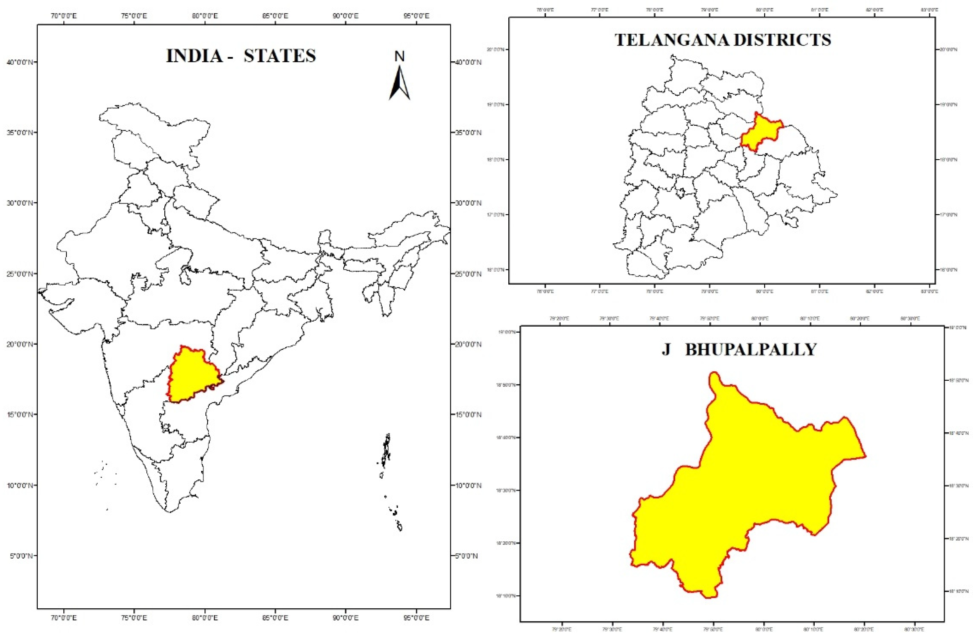
2.1. Study Area

The J Bhupalpally District in Telangana state of India was selected as the study area for this research work. This district lies between latitudes 18°9′10.312″ N and 18°52′13.835″ N and longitudes 79°33′27.045″ E and 80°20′57.83″ E. This district covers an area of 2293 Sq. Km spanning over 223 villages. The map of the study area is shown in Figure 1.

2.2. Datasets

In this research work, temporal data were acquired from Sentinel 2A/2B remote sensing satellites. Among the wide range of products, the dataset with Bottom of Atmosphere (BOA) reflectance has been utilised for this study. In other words, the atmospherically corrected Level-2 product was considered [39]. A total of 12 imageries were acquired for the period ranging from June 2019 to February 2020 as shown in

Table 1. List of Sentinel 2 Temporal datasets used in the study.

Study Site	Sentinel 2A (L2A Product)	Sentinel 2B (L2A Product)
J Bhupalpally District (Telangana)	13 June2019	18 July 2019
	10 November 2019	15 November 2019
	20 December 2019	25 November 2019
	30 December 2019	15 December 2019
	18 February 2020	24 January 2020
		13 February 2020
		23 February 2020

.

The band details of the MSI sensor onboard Sentinel 2 that were used for the study are shown in

Table 2. Bands of MSI sensor onboard Sentinel 2 used in the study.

Band Details	Resolution
Band 2-Blue (490 nm)	10 m
Band 3-Green (560 nm)	10 m
Band 4-Red (665 nm)	10 m
Band 5-Red edge (705 nm)	20 m
Band 6-Red edge (740 nm)	20 m
Band 7-Red edge (783 nm)	20 m
Band 8-NIR (842 nm)	10 m
Band 8A-Red Edge (865 nm)	20 m
Band 11-SWIR (1610 nm)	20 m
Band 12-SWIR (2190 nm)	20 m

.

3. Methods

3.1. Possibilistic c-Means Algorithm (PCM)

The Possibilistic c-means algorithm (PCM) was introduced by Krishnapuram and Keller [35] to deal with the short comings of fuzzy c-means algorithm. This approach is best suited for specific crop mapping as the untrained classes do not affect the classified output, thereby facilitating single-class extraction. The objective function of the PCM classifier is given in Equation (1):

$$J_{pcm}\left(U,V\right)={\displaystyle \sum }_{i=1}^c{\displaystyle \sum }_{k=1}^N{\mu }_k{}_i^{m}D\left(x_k{v}_i\right)+{\displaystyle \sum }_{i=1}^c{\eta }_i{\displaystyle \sum }_{k=1}^N(1-{\mu }_k{}_i)^m$$

(1)

The function is subject to below shown constraints (Equations (2)–(4))

$$\stackrel{max}{\overbrace{i}}{\mu }_{ki}>0ꓯk$$

(2)

$$N<{\sum }_{k=1}^N{\mu }_{ki}>0 \mathrm{for}$$

(3)

$$0\le {\mu }_{ki}\le 1 ꓯ k, i$$

(4)

where,

$‘{\eta }_i’$ is any suitable positive number,

‘$m$’ is called fuzzifier or weighted exponent, $1<m<\infty$.

According to the first term of Equation (2), the separation between feature vector and prototype vector should be as low as possible, while the second term (Equation (2)) forces the membership value to be as high as possible. In PCM, as ‘m’ increases, the possibility of pure pixels occurring in a class decreases [40]. From Equation (2), the membership values for PCM can be estimated as shown in Equation (5);

$$\overline{{\mu }_{ki}}=\frac{1}{1+{\left(\frac{D(x_k,\overline{v_i}}{{\eta }_i}\right)}^{\frac{1}{m-1}}}$$

(5)

where ${\eta }_i$ can be estimated as Equation (6):

$${\eta }_i=K\times \frac{{\sum }_{k=1}^N{\mu }_{ki}^{m}D\left(x_k, \overline{v_i}\right) }{{\sum }_{k=1}^N{\mu }_{ki}^m}$$

(6)

where,

$K$ = 1, constant,

${\eta }_{i }$ is called band width parameter and it is basically a distance at which membership to a class is equal to 0.5.

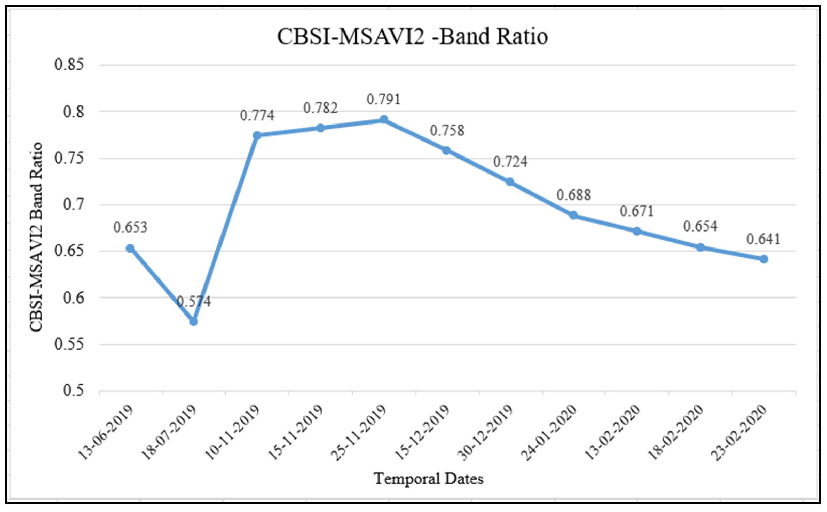
3.2. CBSI-MSAVI2 Indices

This research work proposes a novel approach of using Class-Based Sensor Independent Modified Soil Adjusted Vegetation Index 2 (CBSI-MSAVI2) for the dimensionality reduction. The usage of CBSI-MSAVI2 index ensures maximum enhancement of the target crop, without the need for a deeper knowledge of the sensor specifications. In addition to this, the usage of CBSI-MSAVI2 index ensures the spectral dimensionality reduction while preserving the temporal dimensionality. The formula used to calculate CBSI-MSAVI2 is mentioned in Equation (7), where ${\rho }_{max}$ and ${\rho }_{min}$ denotes maximum and minimum reflectance values. The bands NIR and Red in the calculation of MSAVI2 [41] have been replaced with ${\rho }_{max}$ and ${\rho }_{min}$.

$$CBSI-MSAVI2=\frac{2\left({\rho }_{max}\right)+1-\sqrt{{\left(2\left({\rho }_{max}\right)+1\right)}^2-8{\left({\rho }_{max}-{\rho }_{min}\right)}^2}}{2}$$

(7)

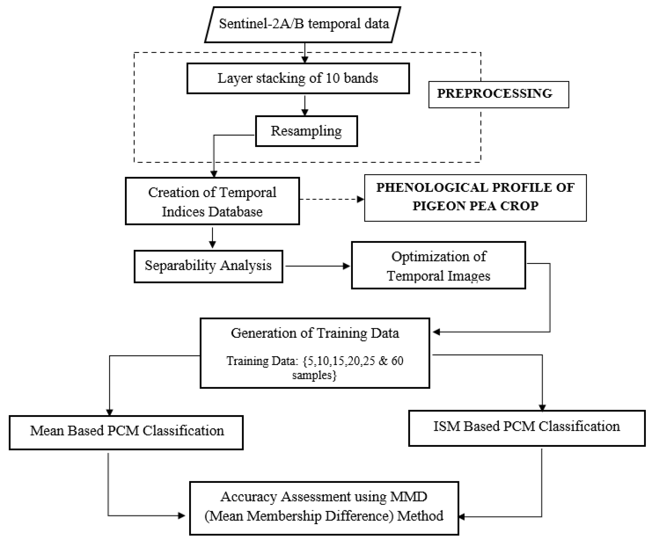
3.3. Methodology Adopted

The temporal data acquired over the period were subjected to preprocessing, where only the required ten bands (mentioned in Table 2) were considered and resampled to 10 m spatial resolution. These resampled data were taken as the input for temporal indices database generation. Initially, various vegetation indices were applied on the dataset to reduce the spectral dimensionality while retaining the temporal dimensionality. Different band combinations considered for generating those indices are maximum and minimum reflectance bands for CBSI-MSAVI2, NIR and Red for MSAVI2 [41] and NIR and Red Edge1 band to generate MSAVI2RE1 [42].

Separability Analysis was carried out on these temporal indices databases to determine the optimal number of temporal images. Since CBSI-MSAVI2 index produced the maximum Euclidean separation distance of Pigeon Pea with respect to the other crops in the region like Cotton, this index was chosen for further classification. The optimal dates were chosen based on the maximum unique information extracted towards Pigeon Pea phenology. The selected temporal dates from the temporal indices database were layer stacked and converted to the Generic Binary format which is compatible with the in-house Java-based Subpixel Multispectral Image Classifier (SMIC) tool [43].

Using this layer stacked input dataset, different signature samples were created ranging from 5 sample points up to 60 points to study the effect of sample size on the classification. The sampling was carried out six times in order to generate the signature files with 5, 10, 15, 20, 25 and 60 samples. The Java-based in-house SMIC tool was used for the PCM classification. In addition to the conventional PCM classification where Mean is taken as the input parameter [44], Individual Samples as Mean (ISM) based PCM classification was also carried out by means of this tool. In this approach, the entire sample is taken as the input parameter instead of considering the statistical mean.

The effect of training concept was experimented by making use of the same signature data of training samples without any kind of alteration. The accuracy assessment was conducted using the Mean Membership Difference (MMD) method. Basically, the difference of mean of membership values of the test fields (Cotton and Pigeon Pea) was calculated with respect to the training fields (Pigeon Pea crop). The methodology followed in this research work is shown in Figure 2.

4. Results& Discussion

4.1. Database of Generated Temporal Indices—CBSI-MSAVI2

The maximum separation distance of the target Pigeon Pea crop was obtained only from the temporal CBSI-MSAVI2 database, thereby making it the most suitable index for this study. In the study [45], it was shown that the Class-Based Sensor Independent Approach is simpler and better for the extraction of single class. This research work proposes a novel Class-Based Sensor Independent-Modified Soil Adjusted Vegetation Index (CBSI-MSAVI2) approach for spectral dimensionality reduction while preserving the temporal dimensionality. The usage of the CBSI-MSAVI2 index ensures maximum enhancement of the target Pigeon Pea crop class, without the need for a deeper knowledge regarding the sensor bands. The in-house SMIC tool was used to generate this index. The different bands as maximum and minimum reflectance used in CBSI-MSAVI2 of the temporal images were shown in

Table 3. CBSI-MSAVI2—Maximum and Minimum Reflectance Bands for Temporal indices that ensure maximum enhancement of the target Pigeon Pea crop class.

Date	Minimum Band	Maximum Band
13 June 2019	Band 2—Blue	Band 11—SWIR
18 July 2019	Band 2—Blue	Band 8A—Red Edge
10 November 2019	Band 2—Blue	Band 7—Red Edge
15 November 2019	Band 2—Blue	Band 8A—Red Edge
25 November	Band 2—Blue	Band 8A—Red Edge
15 December 2019	Band 2—Blue	Band 8A—Red Edge
30 December 2019	Band 2—Blue	Band 8A—Red Edge
24 January 2020	Band 2—Blue	Band 11—SWIR
13 February 2020	Band 2—Blue	Band 11—SWIR
18 February 2020	Band 2—Blue	Band 11—SWIR
23 February 2020	Band 2—Blue	Band 11—SWIR

.

The band ratios computed at each of the temporal dates are shown in the Figure 3.

The band ratio (0.791) peaks in the month of November indicating the peak of the crop growth. Gradually, the ratio decreases over the months January–February, coinciding with the harvest period. Hence, the growth cycle of the Pigeon Pea crop is better modelled using CBSI-MSAVI2.

4.2. Separability Analysis and Selection of Optimal Dates

The separability analysis was carried out for the target crop, Pigeon Pea with other vegetation patches, plantation and the Cotton crop grown in the study area, to find out optimum number of dates. Out of all the indices used, the CBSI-MSAVI2 produced the maximum Euclidean Separation of Cotton [46], and had also produced the highest Euclidean separation on using the Class Based Sensor Independent index. Basically, the Euclidean separation distance between the Pigeon Pea crop and the other crops has been maximised, starting with single date indices data to reduce the spectral overlap. Once the separation distance starts getting constant, the optimum dates were selected from that point. This way, the selected optimum dates ensure the maximum extraction of Pigeon Pea phenology for the best results. The result of separability analysis for CBSI-MSAVI2 has been shown in

Table 4. Separability analysis using CBSI-MSAVI2 temporal indices images for the selection of best temporal dates to map Pigeon Pea crop with spectrally least similar cotton crop.

No. of Images	Date Combinations	Min Separability Distance
1	5	15
2	2, 5	40
3	1, 2, 5	47
4	1, 2, 4, 5	54
5	1, 2, 4, 5, 8	57
6	1, 2, 4, 5, 8, 10	59
7	1, 2, 3, 4, 5, 8, 10	60
8	1, 2, 3, 4, 5, 7, 8, 10	60
9	1, 2, 3, 4, 5, 7, 8, 9, 10	60
10	1, 2, 3, 4, 5, 6, 7, 8, 9, 10	60

Note: Selected dates 1, 2, 3, 4, 5, 6, 7, 8, 9 and 10 correspond to 13 June (2019), 18 July (2019), 10 November (2019), 25 November (2019), 15 December (2019), 30 December (2019), 24 January (2020), 13 February (2020), 18 February (2020) and 23 February (2020). It has been found Cotton crop was spectrally close to Pigeon Pea crop, we tried to keep it spectrally far using optimized temporal indices database.

.

A closer look at Table 4 reveals the fact that the separability distance becomes almost constant at 59–60. This value was attained while taking six date temporal image combinations. Hence the dates corresponding to the number of temporal images (6) are the optimum dates, which are: 13 June (2019), 18 July (2019), 25 November (2019), 15 December (2019), 13 February (2020) and 23 February (2020) from Table 4. In other words, these dates capture the unique phenological information of the target Pigeon Pea crop to its maximum extent, which is helpful for the level-2 classification.

4.3. Optimising Weighted Exponent (m) Parameter

The value of “m” was varied from 1.1 to 3 to determine the optimised value to be used for the classification. For each of the outputs obtained by varying the value of m, MMD analysis was carried out to find the best result. The results were analysed by comparing the membership values of Pigeon Pea training fields with those of Pigeon Pea and Cotton Test fields. This is a two-pronged approach of examining the difference in membership values within the Pigeon Pea field and the extent of separation achieved with respect to the spectrally similar Cotton crop. The performance of the classification has not only been judged by the proximity of the Pigeon Pea training fields to the Pigeon Pea test fields, but also with the departure attained from the Cotton test fields, as this was spectrally closest crop to Pigeon Pea crop. As ‘m’ increases the chances of occurrence fuzziness in the output increases. In other words, when the value of m is closer to 1, it indicates a hard classification output. The research work [47], which had used a Possibilistic c-means classifier with a hypertangent (tanh) kernel for wheat (Triticum aestivum) identification, evaluated that for 2.7, 2.5, and 2.5 values of the weighted constant (m), images of 4 date combinations from Formosat-2 and Landsat-8 (Operational Land Imager) sensors represent the nicely separated wheat crop from other vegetation.

It was noted that the difference in the membership value remained almost constant in the case of spectrally similar Cotton for an ‘m’ value of 2.1. On the other hand, the MMD value for Pigeon Pea remained closer to 0. Thus, the optimised m value used for PCM classification was 2.1. The table of MMD values against the chosen “m” for Pigeon Pea and Cotton are shown in

Table 5. Varying ‘m’ values with MMD exhibiting Proximity of Pigeon Pea Training Fields to the Pigeon Pea Test Fields—Mean training parameter based PCM classifier.

‘M’ Value	Membership Values from Testing Site—Pigeon Pea						Mean Value at Test Site	Mean Value at Training Site	MMD
	1	2	3	4	5	6
1.1	0.996078	0.996078	0.996078	0.996078	0.996078	0.992157	0.995425	0.99607843	0.000654
1.5	0.992157	0.992157	0.996078	0.996078	0.996078	0.992157	0.994118	0.99542484	0.001307
2.0	0.937255	0.945098	0.956863	0.945098	0.941176	0.945098	0.945098	0.94705882	0.001961
2.1	0.921569	0.929412	0.941176	0.929412	0.92549	0.941176	0.931373	0.93202614	0.000654
2.2	0.905882	0.917647	0.929412	0.917647	0.909804	0.92549	0.917647	0.91830065	0.000654
2.3	0.890196	0.901961	0.913725	0.901961	0.894118	0.901961	0.900654	0.90261438	0.001961
2.4	0.870588	0.890196	0.886275	0.909804	0.866667	0.886275	0.884967	0.88823529	0.003268
2.5	0.854902	0.870588	0.866667	0.898039	0.85098	0.870588	0.868627	0.87385621	0.005229
2.6	0.839216	0.835294	0.858824	0.882353	0.835294	0.854902	0.85098	0.85947712	0.008497
2.7	0.827451	0.819608	0.843137	0.870588	0.823529	0.843137	0.837908	0.84705882	0.00915
2.8	0.811765	0.807843	0.831373	0.858824	0.811765	0.831373	0.82549	0.83398693	0.008497
2.9	0.8	0.796078	0.819608	0.847059	0.8	0.819608	0.813725	0.82156863	0.007843
3.0	0.788235	0.784314	0.807843	0.835294	0.788235	0.807843	0.801961	0.81111111	0.00915

and

Table 6. Varying ‘m’ values with MMD exhibiting Proximity of Pigeon Pea Training Fields to the Pigeon Pea Test Fields—ISM training parameter based PCM classifier.

‘M’ Value	Membership Values from Testing Site—Pigeon Pea						Mean Value at Test Site	Mean Value at Training Site	MMD
	1	2	3	4	5	6
1.1	0.996078	0.996078	0.996078	0.996078	0.996078	0.996078	0.996078	0.996078	0
1.5	0.976471	0.976471	0.980392	0.976471	0.980392	0.976471	0.977778	0.976471	0.001307
2.0	0.87451	0.866667	0.878431	0.870588	0.870588	0.866667	0.871242	0.869281	0.001961
2.1	0.854902	0.847059	0.858824	0.85098	0.85098	0.847059	0.851634	0.84902	0.002614
2.2	0.835294	0.827451	0.839216	0.831373	0.831373	0.827451	0.832026	0.830065	0.001961
2.3	0.815686	0.807843	0.823529	0.811765	0.811765	0.811765	0.813725	0.810458	0.003268
2.4	0.8	0.792157	0.803922	0.796078	0.796078	0.792157	0.796732	0.794771	0.001961
2.5	0.784314	0.776471	0.788235	0.780392	0.788235	0.780392	0.783007	0.779085	0.003922
2.6	0.768627	0.764706	0.776471	0.764706	0.764706	0.764706	0.76732	0.766013	0.001307
2.7	0.756863	0.74902	0.760784	0.752941	0.752941	0.752941	0.754248	0.752288	0.001961
2.8	0.745098	0.737255	0.74902	0.741176	0.741176	0.741176	0.742484	0.74183	0.000654
2.9	0.733333	0.729412	0.741176	0.729412	0.729412	0.729412	0.732026	0.730719	0.001307
3.0	0.72549	0.717647	0.729412	0.721569	0.721569	0.717647	0.722222	0.720261	0.001961

and

Table 7. Varying ‘m’ values with MMD exhibiting Departure of Pigeon Pea Training Fields from the Cotton Test Fields—Mean training parameter based PCM classifier.

‘M’ Value	Membership Values from Testing Site—Cotton						Mean Value at Test Site	Mean Value at Training Site	MMD
	1	2	3	4	5	6
1.1	0.011765	0.015686	0.019608	0.019608	0.011765	0.019608	0.01634	0.996078431	0.979739
1.5	0.298039	0.309804	0.313725	0.313725	0.290196	0.317647	0.30719	0.995424837	0.688235
2.0	0.392157	0.4	0.4	0.4	0.388235	0.403922	0.397386	0.947058824	0.549673
2.1	0.403922	0.407843	0.411765	0.411765	0.4	0.415686	0.408497	0.932026144	0.523529
2.2	0.411765	0.415686	0.415686	0.415686	0.407843	0.419608	0.414379	0.918300654	0.503922
2.3	0.415686	0.423529	0.423529	0.423529	0.415686	0.427451	0.421569	0.902614379	0.481046
2.4	0.423529	0.427451	0.427451	0.427451	0.419608	0.431373	0.426144	0.888235294	0.462092
2.5	0.427451	0.431373	0.435294	0.435294	0.423529	0.435294	0.431373	0.873856209	0.442484
2.6	0.431373	0.435294	0.439216	0.439216	0.431373	0.439216	0.435948	0.859477124	0.423529
2.7	0.435294	0.439216	0.439216	0.439216	0.435294	0.443137	0.438562	0.847058824	0.408497
2.8	0.439216	0.443137	0.443137	0.443137	0.435294	0.447059	0.44183	0.833986928	0.392157
2.9	0.443137	0.447059	0.447059	0.447059	0.439216	0.45098	0.445752	0.821568627	0.375817
3.0	0.443137	0.45098	0.45098	0.45098	0.443137	0.45098	0.448366	0.811111111	0.362745

and

Table 8. Varying ‘m’ values with MMD exhibiting Departure of Pigeon Pea Training Fields from the Cotton Test Fields—ISM training parameter based PCM classifier.

‘M’ Value	Membership Values from Testing Site—Cotton						Mean Value at Test Site	Mean Value at Training Site	MMD
	1	2	3	4	5	6
1.1	0.003922	0.007843	0.003922	0.003922	0.003922	0.003922	0.004575	0.996078	0.991503
1.5	0.270588	0.278431	0.270588	0.270588	0.258824	0.278431	0.271242	0.976471	0.705229
2.0	0.380392	0.380392	0.380392	0.380392	0.372549	0.380392	0.379085	0.869281	0.490196
2.1	0.388235	0.392157	0.388235	0.388235	0.384314	0.392157	0.388889	0.84902	0.460131
2.2	0.396078	0.4	0.396078	0.396078	0.392157	0.4	0.396732	0.830065	0.433333
2.3	0.403922	0.407843	0.403922	0.403922	0.4	0.407843	0.404575	0.810458	0.405882
2.4	0.411765	0.415686	0.411765	0.411765	0.407843	0.415686	0.412418	0.794771	0.382353
2.5	0.415686	0.419608	0.419608	0.419608	0.411765	0.419608	0.417647	0.779085	0.361438
2.6	0.423529	0.423529	0.423529	0.423529	0.419608	0.423529	0.422876	0.766013	0.343137
2.7	0.427451	0.427451	0.427451	0.427451	0.423529	0.427451	0.426797	0.752288	0.32549
2.8	0.431373	0.431373	0.431373	0.431373	0.427451	0.431373	0.430719	0.74183	0.311111
2.9	0.435294	0.435294	0.435294	0.435294	0.431373	0.435294	0.434641	0.730719	0.296078
3.0	0.439216	0.439216	0.439216	0.439216	0.435294	0.439216	0.438562	0.720261	0.281699

, respectively. Thus, the membership values attained at both Pigeon Pea test fields and Cotton test fields were compared with the membership values at training fields of Pigeon Pea in order to get an insight into the respective proximity and separation achieved by the classification.

4.4. Classification Results

The objective of this research was to study the effect of the training concept and the sample size in classification meant for specific Pigeon Pea crop mapping. The effect of the training concept incorporates “Individual Samples” directly to be taken as the mean input parameter without going with the conventional “mean”. With regard to this, six training sample data were generated, consisting of 5, 10, 15, 20, 25 and 60 training sample points. In general classification, according to [48],“10*n” samples size have to be considered for training, ‘n’ being the number of bands in the input image. Here, since 6 optimum dates were chosen, according to the 10*n rule, meaning 10*6, i.e., 60 samples needed to be chosen for training purpose. The subset image taken is shown in Figure 4 and the classification results for the signature file (5 samples—minimum) with the two different training parameters are shown in Figure 5.

4.5. Accuracy Assessment Using MMD

The Mean Membership Difference (MMD) method has been used to quantitatively analyze the output images generated. Basically, the difference of the mean of membership values of the test fields (Cotton and Pigeon Pea) with training fields were calculated with respect to the training fields of the Pigeon Pea crop. It is expected that the MMD for Pigeon Pea test fields were closer to 0 (proximity) and that of the Cotton fields were tending towards 1 (separation). This two-pronged approach of studying the MMD values from the perspectives of Proximity and Separation helps in a better comprehension and evaluation of the classifier performance. The MMD values for the Pigeon Pea Test field while using different training data with various sample sizes using a Mean PCM were shown in

Table 9. Effect of increase in sample size by comparing membership values between Pigeon Pea Training fields and Pigeon Pea Test fields for proximity—Mean training parameter based PCM classifier.

Number of Samples	Membership Values from Testing Site—Pigeon Pea						Mean Value at Test Site	Mean Value at Training Site	MMD	Variance
	1	2	3	4	5	6
5	0.960784	0.956863	0.980392	0.968627	0.960784	0.976471	0.96732	0.968409586	0.019608	0.019172
10	0.956863	0.956863	0.980392	0.964706	0.956863	0.976471	0.965359	0.966775599	0.018954	0.024074
15	0.964706	0.960784	0.984314	0.968627	0.964706	0.980392	0.970588	0.971568627	0.017647	0.019281
20	0.968627	0.964706	0.984314	0.972549	0.968627	0.980392	0.973203	0.973965142	0.016993	0.012309
25	0.972549	0.964706	0.988235	0.976471	0.972549	0.984314	0.976471	0.977124183	0.015686	0.015686
60	0.980392	0.972549	0.988235	0.984314	0.984314	0.992157	0.98366	0.984204793	0.013072	0.019695

, while considering an optimum m value of 2.1.

It was observed that the MMD value ranges between 0.013–0.019 while varying the number of samples. The least MMD value was achieved while using 60 samples. The MMD values for Cotton Test fields from Mean PCM outputs is shown in

Table 10. Effect of increase in sample size by Comparing Membership values between Pigeon Pea Training fields and Cotton Test fields for separation—Mean training parameter based PCM classifier.

Number of Samples	Membership Values from Testing Site—Cotton						Mean Value at Test Site	Mean Value at Training Site	MMD
	1	2	3	4	5	6
5	0.705882	0.670588	0.705882	0.682353	0.603922	0.643137	0.668627	0.968409586	0.318301
10	0.705882	0.670588	0.705882	0.682353	0.603922	0.643137	0.668627	0.966775599	0.315686
15	0.701961	0.666667	0.701961	0.682353	0.603922	0.639216	0.666013	0.971568627	0.322222
20	0.698039	0.662745	0.698039	0.678431	0.6	0.639216	0.662745	0.973965142	0.327451
25	0.694118	0.658824	0.694118	0.670588	0.592157	0.635294	0.657516	0.977124183	0.334641
60	0.701961	0.666667	0.705882	0.682353	0.603922	0.639216	0.666667	0.984204793	0.330065

, while considering optimum m value of 2.1.

The MMD value for Cotton fields ranges from 0.31 to 0.33 for using different sample signature files. The results of the MMD for the Pigeon Pea test fields using an ISM–PCM classification are mentioned in

Table 11. Effect of increase in sample size by comparing membership values between Pigeon Pea Training fields and Pigeon Pea Test fields for proximity—ISM training parameter based PCM classifier.

Number of Samples	Membership Values from Testing Site—Pigeon Pea						Mean Value at Test Site	Mean Value at Training Site	MMD	Variance
	1	2	3	4	5	6
5	0.964706	0.952941	0.976471	0.968627	0.972549	0.984314	0.969935	0.994118	0.024183	0.024401
10	0.968627	0.988235	0.980392	0.980392	0.980392	0.976471	0.979085	1	0.020915	0.008388
15	0.968627	0.988235	0.980392	0.980392	0.980392	0.976471	0.979085	0.996732	0.017647	0.008715
20	0.968627	0.988235	0.980392	0.980392	0.980392	0.976471	0.979085	0.996732	0.017647	0.008715
25	0.980392	0.972549	0.988235	0.984314	0.984314	0.992157	0.98366	1	0.01634	0.009695
60	0.980392	0.972549	0.988235	0.984314	0.984314	0.992157	0.98366	1	0.01634	0.009695

, while considering an optimum m value of 2.1.

The comparison of the variance values against sample size for both the approaches is mentioned in Figure 6.

While using the ISM approach, the variance of the Pigeon Pea test field varies from 0.008–0.02, which is lesser when compared to the conventional Mean PCM. This shows that the heterogeneity within the fields was handled better using this approach. The MMD values for Cotton field using the ISM–PCM classification is shown in

Table 12. Effect of increase in sample size by comparing membership values between Pigeon Pea Training fields and Cotton Test fields for separation—ISM training parameter based PCM classifier.

Number of Samples	Membership Values from Testing Site—Cotton						Mean Value at Test Site	Mean Value at Training Site	MMD
	1	2	3	4	5	6
5	0.670588	0.643137	0.678431	0.658824	0.588235	0.619608	0.643137	0.994118	0.35098
10	0.654902	0.694118	0.647059	0.65098	0.717647	0.643137	0.667974	1	0.332026
15	0.643137	0.686275	0.643137	0.639216	0.713725	0.635294	0.660131	0.996732	0.336601
20	0.643137	0.686275	0.643137	0.639216	0.713725	0.635294	0.660131	0.996732	0.336601
25	0.72549	0.690196	0.733333	0.705882	0.627451	0.658824	0.690196	1	0.309804
60	0.72549	0.690196	0.733333	0.705882	0.627451	0.658824	0.690196	1	0.309804

, while considering an optimum m value of 2.1.

The MMD value for Cotton ranges from 0.30–0.35, which is slightly better when compared to the values obtained using the conventional Mean PCM, thereby exhibiting a better separation from Pigeon Pea. It was observed that as the sample size kept increasing, the MMD value for the Pigeon Pea test fields also kept decreasing. In the case of Cotton, a decrease in MMD values is seen for the ISM approach, whereas there is a steady increase of the same in the conventional approach.

Ref. [49] followed a temporal approach in the specific mapping of Sugarcane Ratoon. Time series data from LISS-III and AWiFS sensors were separately subjected to the Possibilistic c-Means classifier to extract single class sub-pixel information. A Fuzzy Modified Possibilistic c-Means (MPCM) classifier was used by [50] to identify and map the vegetation cover in Newai town of Rajasthan. In this study, data from Sentinel -1 and Sentinel -2 missions were used to fulfil the required temporal dates to incorporate phenological and sessional variation. Thus, the incorporation of dual-sensor data helped in better mapping of the agro-geography. The transplanted paddy crops were mapped using MPCM and Noise Clustering algorithms by [46]. Due to the presence of cloud cover, a single optical sensor was not enough to provide the required temporal scenes. Two optical datasets (Sentinel-2 and Landsat-8) and one SAR dataset (Sentinel-1) were used for this work. The Noise Clustering algorithm had outperformed MPCM in the mapping of transplanted paddy crops.

In all of these works, pixel-based classifiers had used means or variance-covariance statistical parameters generated from training samples. In reality, these statistical parameters do not represent in totality about variations existing within class.

The research work of [50] aimed at the identification of different crops grown in a region by means of the fuzzy PCM algorithm. The MMD attained between two different crops (viz., mustard and wheat) in the study was close to 0.077, thereby indicating very little separation. Although the crops used in [50] are different from that of the current research work, better separation could have been achieved by employing the ISM-based PCM classification. Here in our research work, an MMD of up to 0.35 was attained on using this unique approach.

5. Conclusions

The training parameter concept plays an important role in the classification output. When the individual samples concept was considered as an input training parameter, a better representation of the field was achieved through the PCM classifier. The variance of the MMD values of the Pigeon Pea test fields indicates that the ISM–PCM classification handles heterogeneity in a better way. The variance value achieved in the conventional method was 0.019, whereas that for the ISM approach was 0.008.

Although, general classification requires the presence of a minimum of 60 samples (considering 10*n rule), but the PCM algorithm works well even in the presence of 5 training samples. On increasing the training samples from 5 to 60, the MMD value of the Pigeon Pea test fields kept decreasing from 0.019 to 0.013. Even the MMD values for the Cotton fields showed a decreasing trend with an increase in the number of samples. Since, the variation in MMD values was quite nominal, it can be concluded that the effect of sample size was not significant in the fuzzy PCM classification for MMD values. However, the variance value was decreasing with the increasing sample size, especially in the ISM training approach. This algorithm exhibits a robust performance even in the presence of a minimal number of training samples, say 15 training samples onwards.

References

1. GoI. Annual Report 2018-19. Ministry of Agriculture & Farmers Welfare; Government of India: New Delhi, India, 2019; pp. 1–224.
2. Pigeonpea_E.pdf. Available online: https://farmer.gov.in/imagedefault/Other_Pulses/Pigeonpea_E.pdf (accessed on 19 November 2021).
3. Rosenthal, G. Economic and Social Council. Oxford Handb. United Nations 2008, 00424, 135–148. [Google Scholar] [CrossRef]
4. Xue, Y.; Li, Y.; Guang, J.; Zhang, X.; Guo, J. Small satellite remote sensing and applications—History, current and future. Int. J. Remote Sens. 2008, 29, 4339–4372. [Google Scholar] [CrossRef]
5. Millan, R.M.; von Steiger, R.; Ariel, M.; Bartalev, S.; Borgeaud, M.; Campagnola, S.; Castillo-Rogez, J.C.; Fléron, R.; Gass, V.; Gregorio, A.; et al. Small satellites for space science: A COSPAR scientific roadmap. Adv. Space Res. 2019, 64, 1466–1517. [Google Scholar] [CrossRef]
6. Weiss, M.; Jacob, F.; Duveiller, G. Remote sensing for agricultural applications: A meta-review. Remote Sens. Environ. 2019, 236, 111402. [Google Scholar] [CrossRef]
7. Naik, P.; Kumar, A. A Stochastic Approach for Automatic Collection of Precise Training Data for a Soft Machine Learning Algorithm Using Remote Sensing Images. In Soft Computing for Problem Solving. Advances in Intelligent Systems and Computing; Tiwari, A., Ahuja, K., Yadav, A., Bansal, J.C., Deep, K., Nagar, A.K., Eds.; Springer: Singapore, 2021; Volume 1393, pp. 285–297. [Google Scholar] [CrossRef]
8. Lark, T.; Schelly, I.; Gibbs, H. Accuracy, Bias, and Improvements in Mapping Crops and Cropland across the United States Using the USDA Cropland Data Layer. Remote Sens. 2021, 13, 968. [Google Scholar] [CrossRef]
9. Paliwal, A.; Jain, M. The Accuracy of Self-Reported Crop Yield Estimates and Their Ability to Train Remote Sensing Algorithms. Front. Sustain. Food Syst. 2020, 4, 25. [Google Scholar] [CrossRef] [Green Version]
10. Gong, J.; Sui, H.; Ma, G.; Zhou, Q. A review of multi-temporal remote sensing data change detection algorithm. Int. Arch. Photogramm. Remote Sens. Spat. Inf. Sci.-ISPRS Arch. 2008, 37, 757–762. [Google Scholar]
11. Ghamisi, P.; Rasti, B.; Yokoya, N.; Wang, Q.; Hofle, B.; Bruzzone, L.; Bovolo, F.; Chi, M.; Anders, K.; Gloaguen, R.; et al. Multisource and Multitemporal Data Fusion in Remote Sensing. arXiv 2018, arXiv:1812.08287. [Google Scholar]
12. Naik, P.; Dalponte, M.; Bruzzone, L. A comparison on the use of different satellite multispectral data for the prediction of aboveground biomass. In Image and Signal Processing for Remote Sensing XXVI; International Society for Optics and Photonics: Bellingham, WC, USA, 2020; Volume 11533, p. 1153315. [Google Scholar] [CrossRef]
13. Naik, P.; Dalponte, M.; Bruzzone, L. Prediction of Forest Aboveground Biomass Using Multitemporal Multispectral Remote Sensing Data. Remote Sens. 2021, 13, 1282. [Google Scholar] [CrossRef]
14. Shu, C.; Sun, L. Automatic target recognition method for multitemporal remote sensing image. Open Phys. 2020, 18, 170–181. [Google Scholar] [CrossRef]
15. Yan, S.; Yao, X.; Zhu, D.; Liu, D.; Zhang, L.; Yu, G.; Gao, B.; Yang, J.; Yun, W. Large-scale crop mapping from multi-source optical satellite imageries using machine learning with discrete grids. Int. J. Appl. Earth Obs. Geoinf. 2021, 103, 102485. [Google Scholar] [CrossRef]
16. Sun, C.; Bian, Y.; Zhou, T.; Pan, J. Using of Multi-Source and Multi-Temporal Remote Sensing Data Improves Crop-Type Mapping in the Subtropical Agriculture Region. Sensors 2019, 19, 2401. [Google Scholar] [CrossRef] [PubMed] [Green Version]
17. Pôças, I.; Calera, A.; Campos, I.; Cunha, M. Remote sensing for estimating and mapping single and basal crop coefficientes: A review on spectral vegetation indices approaches. Agric. Water Manag. 2020, 233, 106081. [Google Scholar] [CrossRef]
18. Campos, I.; Gómez, L.G.; Villodre, J.; Calera, M.; Campoy, J.; Jiménez, N.; Plaza, C.; Sánchez-Prieto, S.; Calera, A. Mapping within-field variability in wheat yield and biomass using remote sensing vegetation indices. Precis. Agric. 2018, 20, 214–236. [Google Scholar] [CrossRef]
19. Moumni, A.; Lahrouni, A. Machine Learning-Based Classification for Crop-Type Mapping Using the Fusion of High-Resolution Satellite Imagery in a Semiarid Area. Scientifica 2021, 2021, 8810279. [Google Scholar] [CrossRef] [PubMed]
20. Kumari, M.; Pandey, V.; Choudhary, K.K.; Murthy, C.S. Object-based machine learning approach for soybean mapping using temporal sentinel-1/sentinel-2 data. Geocarto Int. 2021, 1–19. [Google Scholar] [CrossRef]
21. Kobayashi, N.; Tani, H.; Wang, X.; Sonobe, R. Crop classification using spectral indices derived from Sentinel-2A imagery. J. Inf. Telecommun. 2020, 4, 67–90. [Google Scholar] [CrossRef]
22. Viskovic, L.; Kosovic, I.N.; Mastelic, T. Crop Classification using Multi-spectral and Multitemporal Satellite Imagery with Machine Learning. In Proceedings of the 2019 International Conference on Software, Telecommunications and Computer Networks (SoftCOM), Split, Croatia, 19–21 September 2019; p. 8903738. [Google Scholar]
23. Saini, R.; Ghosh, S.K. Crop classsification on single date Sentinel-2 Imagery using Random Forest and Suppor Vector Machine. Int. Arch. Photogramm. Remote Sens. Spat. Inf. Sci. 2018, 42, 683–688. [Google Scholar] [CrossRef] [Green Version]
24. Kamilaris, A.; Prenafeta-Boldú, F.X. Deep learning in agriculture: A survey. Comput. Electron. Agric. 2018, 147, 70–90. [Google Scholar] [CrossRef] [Green Version]
25. Melgani, F.; Bruzzone, L. Classification of hyperspectral remote sensing images with support vector machines. IEEE Trans. Geosci. Remote Sens. 2004, 42, 1778–1790. [Google Scholar] [CrossRef] [Green Version]
26. Fawagreh, K.; Gaber, M.M.; Elyan, E. Random forests: From early developments to recent advancements. Syst. Sci. Control Eng. Open Access J. 2014, 2, 602–609. [Google Scholar] [CrossRef] [Green Version]
27. Liakos, K.G.; Busato, P.; Moshou, D.; Pearson, S.; Bochtis, D. Machine learning in agriculture: A review. Sensors 2018, 18, 2674. [Google Scholar] [CrossRef] [Green Version]
28. Scheer, C.; Guder, L. Deep Learning in Agriculture: A Systematic Literature Review Deep Learning in Agriculture Três de Maio. Bachelor Thesis, Faculty of Três de Maio, Tres de Maio, Brazil, 2019. [Google Scholar] [CrossRef]
29. Saleem, M.H.; Potgieter, J.; Arif, K.M. Automation in Agriculture by Machine and Deep Learning Techniques: A Review of Recent Developments; Springer: New York, NY, USA, 2021; Volume 22. [Google Scholar]
30. Naik, P.; Dalponte, M.; Bruzzone, L. A Disentangled Variational Autoencoder for Prediction of Above Ground Biomass from Hyperspectral Data. In Proceedings of the 2021 IEEE International Geoscience and Remote Sensing Symposium IGARSS, Brussels, Belgium, 11–16 July 2021; pp. 2991–2994. [Google Scholar] [CrossRef]
31. Tilson, L.; Excell, P.; Green, R. A Generalisation of the Fuzzy C-means Clustering Algorithm. In Proceedings of the International Geoscience and Remote Sensing Symposium, Remote Sensing: Moving Toward the 21st Century, Edinburgh, UK, 12–16 September 1988; Volume 3, pp. 1783–1784. [Google Scholar] [CrossRef]
32. Hung, M.-C.; Yang, D.-L. An efficient Fuzzy C-Means clustering algorithm. In Proceedings of the 2001 IEEE International Conference on Data Mining, Maebashi City, Japan, 9–12 December 2002; pp. 225–232. [Google Scholar] [CrossRef]
33. Sandhya, P.; Kumar, A. A Survey on Fuzzy C-means Clustering Techniques. Ijedr 2017, 5, 1151–1155. [Google Scholar]
34. Krishnapuram, R.; Keller, J. The possibilistic C-means algorithm: Insights and recommendations. IEEE Trans. Fuzzy Syst. 1996, 4, 385–393. [Google Scholar] [CrossRef]
35. Singh, A.; Kumar, A.; Upadhyay, P. Modified possibilistic c- means with constraints (MPCM-S) approach for incorporating the local information in a remote sensing image classification. Remote Sens. Appl. Soc. Environ. 2020, 18, 100319. [Google Scholar] [CrossRef]
36. Singh, A.; Kumar, A.; Upadhyay, P. A novel approach to incorporate local information in Possibilistic c-Means algorithm for an optical remote sensing imagery. Egypt. J. Remote Sens. Space Sci. 2020, 24, 151–161. [Google Scholar] [CrossRef]
37. Singh, A.; Kumar, A. Identification of Paddy Stubble Burnt Activities Using Temporal Class-Based Sensor-Independent Indices Database: Modified Possibilistic Fuzzy Classification Approach. J. Indian Soc. Remote Sens. 2019, 48, 423–430. [Google Scholar] [CrossRef]
38. Louis, J. Sentinel 2 MSI—Level 2A Product Definition. Eur. Sp. Agency 2016, 49. Available online: https://sentinel.esa.int/documents/247904/1848117/Sentinel-2-Level-2A-Product-Definition-Document.pdf (accessed on 22 January 2022).
39. Jankowski, J.A. (Ed.) Inflammation and Gastrointestinal Cancers; Springer Science & Business Media: Berlin/Heidelberg, Germany, 2011. [Google Scholar] [CrossRef]
40. Qi, J.; Chehbouni, A.; Huete, A.R.; Kerr, Y.H.; Sorooshian, S. A modified soil adjusted vegetation index. Remote Sens. Environ. 1994, 48, 119–126. [Google Scholar] [CrossRef]
41. Vincent, A.; Kumar, A.; Upadhyay, P. Effect of Red-Edge Region in Fuzzy Classification: A Case Study of Sunflower Crop. J. Indian Soc. Remote Sens. 2020, 48, 645–657. [Google Scholar] [CrossRef]
42. Kumar, A.; Ghosh, S.; Dadhwal, V. ALCM: Automatic land cover mapping. J. Indian Soc. Remote Sens. 2010, 38, 239–245. [Google Scholar] [CrossRef]
43. Krishnapuram, R.; Keller, J. A possibilistic approach to clustering. IEEE Trans. Fuzzy Syst. 1993, 1, 98–110. [Google Scholar] [CrossRef]
44. Upadhyay, P.; Kumar, A.; Roy, P.S.; Ghosh, S.; Gilbert, I. Effect on specific crop mapping using WorldView-2 multispectral add-on bands: Soft classification approach. J. Appl. Remote Sens. 2012, 6, 063524-1. [Google Scholar] [CrossRef]
45. Rawat, A.; Kumar, A.; Upadhyay, P.; Kumar, S. Multisensor temporal approach for transplanted paddy fields mapping using fuzzy-based classifiers. J. Appl. Remote Sens. 2020, 14, 024524. [Google Scholar] [CrossRef]
46. Nandan, R.; Kamboj, A.; Kumar, A.; Kumar, S.; Reddy, K.V. Formosat-2 with Landsat-8 Temporal-Multispectral Data for Wheat Crop Identification using Hypertangent Kernel based Possibilistic classifier. J. Geomat. 2016, 10, 89–95. [Google Scholar]
47. Jensen, J.R.; Lulla, K. Introductory Digital Image Processing: A Remote Sensing Perspective, 3rd ed.; Prentice Hall Series in Geographic Information Science; Pearson Prentice Hall: Upper Saddle River, NJ, USA, 2005; ISBN 0-13-145361-0. [Google Scholar]
48. Misra, G.; Kumar, A.; Patel, N.R.; Zurita-Milla, R. Mapping a Specific Crop—A Temporal Approach for Sugarcane Ratoon. J. Indian Soc. Remote Sens. 2013, 42, 325–334. [Google Scholar] [CrossRef]
49. Devinda, C.S.; Kumar, A. Application of fuzzy machine learning algorithm in agro-geography. Khoj Int. Peer Rev. J. Geogr. 2020, 7, 30–46. [Google Scholar] [CrossRef]
50. Najafabadi, M.M.; Villanustre, F.; Khoshgoftaar, T.M.; Seliya, N.; Wald, R.; Muharemagic, E. Deep learning applications and challenges in big data analytics. J. Big Data 2015, 2, 1. [Google Scholar] [CrossRef] [Green Version]
Figure 1. Study Area for Pigeon Pea crop identification, J Bhupalpally District, Telangana state, India.
Geomatics 02 00007 g001
Figure 2. Proposed Methodology of research work.
Geomatics 02 00007 g002
Figure 3. Graph of CBSI-MSAVI2 indices versus temporal dates.
Geomatics 02 00007 g003
Figure 4. Subset image from district image, dated 10 November 2019.
Geomatics 02 00007 g004
Figure 5. PCM Classification output with five samples signature file, (a) conventional mean PCM output (b) ISM based PCM output.
Geomatics 02 00007 g005
Figure 6. Graph of variance versus sample size for both the approaches.
Geomatics 02 00007 g006