


Abstract
Since the 1930s, theories of skin-friction drag from plates with rough surfaces have been based by analogy to turbulent flow in pipes with rough interiors. Failure of this analogy at small fluid velocities has frustrated attempts to create a comprehensive theory. Utilizing the concept of a self-similar roughness that disrupts the boundary layer at all scales, this investigation derives formulas for a rough or smooth plate’s skin-friction coefficient and forced convection heat transfer given its characteristic length, root-mean-squared (RMS) height-of-roughness, isotropic spatial period, Reynolds number, and the fluid’s Prandtl number. This novel theory was tested with 456 heat transfer and friction measurements in 32 data-sets from one book, six peer-reviewed studies, and the present apparatus. Compared with the present theory, the RMS relative error (RMSRE) values of the 32 data-sets span 0.75% through 8.2%, with only four data-sets exceeding 6%. Prior work formulas have smaller RMSRE on only four of the data-sets.
1. Introduction
Fluid flowing along a wall (plate) experiences “skin-friction drag” (or “resistance”) opposing its flow. Related to skin-friction, “forced convection heat transfer” is the heat transfer to or from a surface induced by fluid flow along that surface. Skin-friction and forced convection are fundamental processes with applications from engineering to geophysics.
This investigation seeks to develop formulas to predict the skin-friction coefficient and forced convection heat transfer from rough and smooth plates.
1.1. Pipe-Plate Analogy
Circa 1930, Prandtl [1] and von Kármán [2] developed theories for resistance along (smooth) plates from the results of research on flow through pipes; this is the “pipe-plate analogy”.
In 1934, Prandtl and Schlichting [3] developed a theory of skin-friction resistance for rough plates based on their analysis of Nikuradse’s [4] measurements of sand glued inside pipes (“sand-roughness”). The conclusion of the (translated) paper states:
“The resistance law just derived for rough plates has chiefly validity for a very specific type of roughness, namely a smooth surface to which sand grains have been densely attached and where the Nikuradse pipe results have been taken as the basis…
A single roughness parameter (the relative roughness) will in all likelihood no longer answer the purpose in continued investigations of the roughness problem”.
In 1936, Schlichting [5] investigated the velocity profiles and resistance of water flowing through a closed rectangular channel having one wall replaced in turn by a series of plates, each having an array of identical protrusions attached: spheres, spherical caps (bumps), or cones. The protrusions were positioned on the plates in a hexagonal array that was elongated 15% in the direction of flow.
With a significant pressure drop between inflow and outflow of the channel, it was not an instance of the isobaric (uniform pressure) flow that can occur along external plates. The similarity of channel and pipe flows is well known, but neither supports nor refutes treating rough pipe interiors and plates analogously.
In 1954, Hama [6] described three challenges of the pipe-plate analogy:
“Now there is no obvious reason why pipe flow and boundary-layer flow should be identical or even similar. First, a pressure gradient is essential for flow through a pipe but not along a plate. Second, pipe flow is confined and perforce uniform, while flow along a plate develops semi-freely and bears no such a priori guarantee of displaying similar velocity profiles at successive sections. Finally, the diameter and roughness size are the only geometrical dimensions of established flow in pipes, whereas at least three linear quantities are necessary to characterize the boundary-layer”.
1.2. Boundary Layer
Schlichting [7] describes the boundary layer: “In that thin layer the velocity of the fluid increases from zero at the wall (no slip) to its full value which corresponds to external frictionless flow”.
Hama attempted to confirm the rough pipe-plate analogy with measurements of wire screens affixed to smooth plates, but concluded that it was confirmed only in the fully rough regime (defined below).
1.3. Sand-Roughness
Prior works [3,4,5,6,7,8,9,10,11] specify sand-roughness , the height of “coarse and tightly placed roughness elements such as, for example, coarse sand grains glued on the surface” (Schlichting [7]).
Testing a machined analogue of sand-roughness circa 1975, Pimenta, Moffat, and Kays [8] stated that, while agreement with the Prandtl–Schlichting model was “rather good” in the fully rough regime, the apparatus’s behavior differed from “Nikuradse’s sand-grain pipe flows in the transition region”.
Modeling the wake component of the velocity profile, in 1985 Mills and Hang [9] presented a formula improving the match with data from Pimenta et al. in the rough regime; however, it did not address other flow regimes.
1.4. Flow Regimes
Along with laminar flow, the theory for flow within pipes (and channels) distinguishes three turbulent flow regimes: smooth, (fully) rough, and transitional. Smooth-regime pipe flow encounters viscous resistance varying inversely with the fluid velocity per viscosity ratio. Rough pipe flow encounters resistance varying with the height-of-roughness, while being largely insensitive to viscosity. The transitional regime describes the range of fluid velocities where both viscosity and roughness affect the resistance (Colebrook [12]).
1.5. Reynolds Number
The Reynolds number () represents the bulk fluid velocity (far from the plate); with a subscript represents other fluid velocities. The local Reynolds number , where x is the distance from the leading edge of the plate in the direction of flow, and characteristic length L is the length scale for the physical system. Local measurements are made at distance x from the leading edge. Unless stated otherwise, L is the plate length in the direction of flow.
1.6. Skin-Friction Coefficient
Skin-friction in prior works is represented by the (dimensionless) local drag coefficient or , a function of the relative sand-roughness and or a subscripted .
Prandtl and Schlichting [3] specified the boundaries between flow regimes using the “sand-roughness Reynolds number” . For plates, it assigned the boundaries between smooth, transitional, and rough regimes at and . Pimenta et al. [8] gave as the transitional-to-rough boundary.
Figure 1a presents local skin-friction coefficient curves, regime boundaries, and measurements from the Pimenta et al. [8] plate having at . Figure 1b presents the (whole-plate) average skin-friction coefficients with m.
Figure 1.
(a) Local versus [8], (b) Average versus .
1.7. Plate Flow versus Pipe Flow
Schlichting [7] states: “The resistance to flow offered by rough walls [of pipes] is larger than that …for smooth pipes”.
The rough pipe-plate analogy holds that this rule also applies to rough, external plates. For example, the “Prandtl-Schlichting ” curve is never less than the “White (smooth) ” curve in Figure 1a.
The Pimenta et al. measurements are much closer to than they are to . (The Bergstrom, Akinlade, and Tachie [13] local friction coefficient () measurements of woven wire meshes and perforated sheets (present work Section 14) are also much closer to than .) Pimenta et al. [8] and Mills and Hang [9] both designated as the friction coefficient. All three measurements in Figure 1 are less than the smooth regime coefficient . If rough friction is never less than smooth friction, then these measurements must not be in any turbulent flow regime; the remaining alternative is laminar flow. Laminar flow coefficients have a steeper slope than ; yet these measurements are near the constant level predicted by Mills–Hang for the rough regime.
- The pipe-plate analogy fails for roughness because rough skin-friction coefficients can be less than the smooth regime coefficients for external plates, but not inside pipes.
1.8. More Recent Work
With the rough pipe-plate analogy’s failure obscured by the factor of 2, research based on the pipe-plate analogy continued. The 2004 survey article Jiménez [14] did not question the rough pipe-plate analogy, writing: “The theoretical arguments are sound, but the experimental evidence is inconclusive”.
Circa 2005, Bergstrom, Akinlade, and Tachie [13], performed experiments with sandpapers, woven wire meshes, and perforated sheets attached onto a flat plate, reporting that: , where is the displacement thickness and is the 99% velocity boundary layer thickness. As a function of a roughness metric, this formula has no predictive value because both and must be inferred from velocity measurements along the surface under test. Fortunately, Bergstrom et al. included free-stream velocity in their tables, allowing comparisons of their skin-friction data with the present theory.
The 2021 survey article Chung, Hutchins, Schultz, and Flack [15] summarizes studies for predicting the drag, (boundary layer) velocity profiles, or convection from rough walls or pipes in terms of turbulence theory. Several roughness metrics were introduced, however none convert to the “isotropic spatial period” introduced in Section 8 of the present work.
The studies cited by [15] generally rely on turbulence theory, sand-roughness, Prandtl and Schlichting [3], and the pipe-plate analogy. The present theory relies on none of these.
- Sand-roughness’s lack of generality and the failure of the pipe-plate analogy for roughness motivate a fresh theoretical analysis of isobaric flow along a rough plate, an analysis derived from traceable roughness metrics.
- Prior works analyze turbulence in the boundary layer. The central premise of this investigation is that plate roughness disrupts its boundary layer. The present theory does not utilize turbulence theory.
- The present theory is about plates; it has no implications for smooth or rough pipe flow.
1.9. Approach
Flow along flat, smooth plates can be laminar or turbulent with a continuous boundary layer. This investigation uses the term “rough flow” for disrupted boundary layer flow from a rough plate.
Figure 1a,b shows that the skin-friction from smooth and rough plates are substantially different. Roughness disrupts what would otherwise be a viscous sub-layer adjacent to the plate. Lienhard and Lienhard [16] teaches: “Even a small wall roughness can disrupt this thin sublayer, causing a large decrease in the thermal resistance (but also a large increase in the wall shear stress)”.
With a sufficiently large roughness, the nascent boundary layers forming after each disruption will be smaller than the roughness. The momentum can thus transfer directly between the fluid flow and the plate’s roughness. In order for these transfers to constitute most of the skin-friction, there must be no significant pressure gradients acting on the plate. Thus, this approach works only with a thin plate parallel to an isobaric fluid flow. It is not applicable to pipes, for example, because the pressure decreases as fluid flows through a cylindrical pipe.
Shearing stress can be determined from the free-stream velocity, ignoring turbulent velocity perturbations. Thus, the skin-friction can be derived without turbulence theory.
- While understanding the nature of the flow shed by roughness is of theoretical interest, it is not needed for determining the skin-friction coefficient from a very rough surface in an isobaric flow.
1.10. Not Empirical
Empirical theories derive their coefficients from measurements, inheriting the uncertainties from those measurements. Theories developed from first principles derive their coefficients mathematically. For example, Incropera, DeWitt, Bergman, and Lavine [17] gives the thermal conductance of one face of a diameter D disk into a stationary, uniform medium having thermal conductivity k () as . The present theory derives from first principles; it is not empirical. Each formula is tied to aspects of the plate geometry, fluid, and flow.
1.11. Mathematics
Familiarity with calculus is assumed. Computational geometry, probability, self-similar recurrences, the Lambert function, vector-space norms, and Fourier transforms are also employed; each is briefly introduced or illustrated graphically. Differential equations are not explicitly used.
1.12. Overview
After a comparison of roughness metrics in Section 3, a thought experiment about flow along self-similar roughness is solved using computational geometry in Section 5. The resulting skin-friction coefficient formula’s range of validity does not extend to 0 height-of-roughness. However, analyzing the case of a roughness which induces skin-friction midway between that of a self-similar rough surface and that of a smooth surface in Section 6 produces a formula with unprecedented accuracy for smooth plates.
The self-similar roughness was designed to produce the most boundary layer disruption possible within a given RMS height-of-roughness. A self-similar roughness could be fabricated, but measuring its skin-friction could confirm predictions only for self-similar roughness. Instead, Section 7 and Section 8 turn to isotropic, periodic roughness, which applies in many practical use cases. Fourier analysis and computational geometry result in a quantitative test for periodic isotropy which computes the isotropic period from a sufficiently large height map of roughness. Section 8 computationally tests arrays of posts and wells to find the upper/lower area ratio spans which qualify as isotropic, periodic roughness.
Section 9 presents formulas for converting between local and average friction coefficients, and tests them on measurements from Pimenta et al. [8], Churchill [11], and Žukauskas and Šlančiauskas [18].
Section 10 derives formulas for forced convection heat transfer from rough and smooth plates.
Periodicity enables the derivation of formulas for the onset of rough flow from an isotropic, periodic rough surface in Section 11.
Section 12 finds that the skin-friction coefficient of isotropic, periodic roughness is the same as for self-similar roughness, except when the periodic roughness peaks are all co-planar (at the same elevation) plateaus. Plateau roughness is an isotropic, periodic roughness with most of its area at its peak elevation. Section 12 derives a quantitative test for plateau roughness from a height map of roughness. It also develops formulas for the thresholds separating rough flow and turbulent flow along the plate. These thresholds are tested in Section 14 and Section 15.
Section 13 derives formulas for skin-friction coefficients and convection heat transfer from a plateau roughness shedding rough and turbulent flow from regions of the plate separated at the thresholds developed in Section 12.
Section 14 tests the present theory on measurements from Bergstrom et al. [13].
Section 15 tests the present theory on measurements from the present apparatus.
Section 16 analyzes fluid flow along isotropic, periodic roughness at smaller than the rough flow thresholds found in Section 11. This flow strongly resembles the “oscillations […] discovered in the laminar boundary layer along a flat plate” by Schubauer and Skramstad [19]. The present work treats them identically. Although measurements of flows over such small roughnesses are lacking, smooth plate skin-friction measurements from Gebers [20,21] and uniform-wall-temperature convection measurements by Žukauskas and Šlančiauskas [18] support the present theory.
2. Data-Sets and Evaluation
Table 1.
Sources of friction measurements.
Table 2.
Sources of convection measurements.
Rough surface convection measurements were obtained from an apparatus built for this investigation, which measured (whole-plate) average convection heat transfer in air at 93,000. Appendix A describes this apparatus and its measurement methodology. Section 15 presents its measurements.
The Gebers [20,21] skin-friction measurements were captured from a graph in Schlichting [7] by measuring the distance from each point to the graph’s axes, then scaling to the graph’s units using the “Engauge” software (version 12.1). The remaining measurement data-sets were manually entered from tables in the cited works. Several obvious single-digit typographical errors were corrected.
Two non-obvious single digit errors in the text of a prior work are detailed in Section 14.
The transcribed data-sets are available from Supplementary Materials.
RMS Relative Error
The “±” column of Table 1 and Table 2 lists the estimated measurement uncertainties stated by the cited studies. While essential to empirical theories, these estimates are only indicative for non-empirical theories.
Root-mean-squared relative error (RMSRE) provides an objective, quantitative evaluation. It gauges the fit of measurements to function , giving each of the n samples equal weight in Formula (1).
Along with presenting RMSRE, charts in the present work split RMSRE into the bias and scatter components defined in Formula (2). The root-sum-squared (RSS) of bias and scatter is RMSRE.
3. Roughness Metrics
Two established, traceable roughness metrics are the root-mean-squared (RMS) height-of-roughness and the arithmetic-mean height-of-roughness. For an elevation function defined on area A having a convex perimeter, its mean elevation and RMS height-of-roughness are:
The arithmetic-mean height-of-roughness is defined in terms of the same mean elevation Formula (3):
3.1. Sand-Roughness
Modeling sand-roughness grains as diameter spheres sitting in a pool of depth g glue, the mean elevation of a cell of area A containing one sphere is:
With the cell’s RMS height-of-roughness computed from Formula (4), Figure 2 shows versus the ratio of cell area to the sphere’s shadow area, at six glue-levels between 0% and 50% of . Table 3 lists , grain densities, and conversion factors for Nikuradse’s [4] sand coatings, assuming .
Figure 2.
versus cell area of sand-roughness [4].
Table 3.
Nikuradse’s sand coatings at .
3.2. Conversions
Afzal, Seena, and Bushra [26] fitted 5.333 as the RMS to sand-roughness conversion factor , and 6.45 as the arithmetic-mean to sand-roughness conversion factor (both in pipes). is a broad minimum of the curve in Figure 2.
The “” column values in Table 3 (“Nikuradse” in Figure 2) match each other within 2%. The tightest spread on Table 3 data with the arithmetic-mean height-of-roughness exceeds 20%. Thus, sand-roughness correlates an order of magnitude more strongly with RMS than arithmetic-mean height-of-roughness.
Flack, Schultz, Barros, and Kim [27] measured skin-friction from grit-blasted surfaces in a duct, writing “The root-mean-square roughness height is shown to be most strongly correlated with the equivalent sand-roughness height () for the grit-blasted surfaces”.
- Arithmetic-mean height-of-roughness will not be considered further by this investigation.
3.3. Packed Spheres Roughness
The Pimenta et al. [8] plate was composed of 11 layers of closely packed 1.27 mm diameter metal spheres “arranged such that the surface has a regular array of hemispherical roughness elements”. Joined by brazing, there was no pool of glue surrounding the spheres. Shrinking the cell to the sphere’s shadow, , the RMS height-of-roughness of the top half of the 1.27 mm sphere is 0.150 mm. Pimenta et al. gave ; , which matches 0.150 mm within 1%.
- This investigation will use as the RMS to sand-roughness conversion factor.
4. Formulas from Prior Works
Several prior works gave formulas for skin-friction coefficient in the fully rough regime.
4.1. Prandtl and Schlichting
In boundary layer theory [7], Prandtl and Schlichting gave formulas for fully rough local () and plate average () skin-friction coefficient for a rough plate as a function of and , respectively:
4.2. Mills and Hang
4.3. White
White is also the source of widely used formulas for turbulent skin-friction coefficients of a smooth plate:
4.4. Average Coefficient
Mills and Hang [9] derived the average Formula (10) from the local Formula (9) by fitting a curve to the result of a numerical integration such as Formula (13):
The local Formulas (7), (9), and (11) each have a singularity where the expression containing the logarithm is 0. The lower limit of integration () must be large enough to avoid this; but the lower limit is not revealed in the prior works. The averaging Formula (13) is quite sensitive to the lower limit because the largest value of the local formula occurs there.
4.5. Churchill
Churchill [11] compared eight formulas from diverse sources versus the data from Pimenta et al. [8], finding none significantly closer to the measurements than the Mills–Hang local Formula (9).
Section 9 compares the local fully rough regime formulas with measurements from Pimenta et al. [8].
5. Flow over Obstacles
Jiménez [14] wrote “In flows with , the effect of the roughness extends across the boundary layer, and is also variable. There is little left of the original wall-flow dynamics in these flows, which can perhaps be better described as flows over obstacles”.
This investigation focuses first on a case where flow over obstacles dominates the dynamics. It models the shearing stress of flow along a roughness which disrupts that flow at a succession of scales: L, , , , …. While simpler surfaces may produce rough flow, a roughness which disrupts at all these scales surely will.
- This approach departs from prior works because their continuous boundary layer assumption is incompatible with a roughness which repeatedly disrupts boundary layers.
5.1. Profile Roughness
Simpler than surface roughness, profile roughness is nonetheless informative.
Let a “profile roughness” be a function with ; its mean elevation and RMS height-of-roughness are computed similarly to surface roughness :
5.2. Self-Similar Profile Roughness
Let a “self-similar profile roughness” be a profile roughness function such that the RMS height-of-roughness of over an open interval is twice the RMS height-of-roughness of over each half of that interval (leaving out the midpoint).
These x intervals are open (not containing the endpoints); the value for each endpoint contributes to the height-of-roughness of its parent interval, but not to any sub-interval. This definition is designed so that will have the following property:
- The RMS height-of-roughness of over an open interval, divided by the length of that interval will be invariant through its succession of scales.
5.3. Ramp Permutation
An additional constraint is needed to reduce the uncountable variety of possible functions to a manageable number. Experience with self-similar curves suggests a restriction to profile roughnesses, which are permutations of the linear ramp with . Each elevation from 0 to peak height occurs exactly once.
5.4. Self-Similar Ramp Permutation
A self-similar integer sequence from integers allows self-similar behavior to be explored with a finite approximation. Letting constructs a profile roughness from a sequence by .
The following three examples are self-similar ramp-permutation sequences. Each element of the sequence is generated by calling its recurrence function with a sequence index and w, an integer power of 2. Each recursive call divides w by 2, terminating (and returning) when w reaches 1.
Figure 3.
(a) Gray -code profile roughness; (b) wiggliest self-similar roughness; (c) random reversal profile roughness; (d) random reversal ramp surface.
5.5. Cardinality
The goal is to characterize self-similar roughnesses in general. The theory should work for the vast majority of self-similar roughness functions, with few outliers. For a given number of points , there are distinct self-similar ramp-permutation sequences, of which there are only two distinct ramps and two distinct wiggliest sequences.
5.6. Friction Travel and Velocity
When the fluid flow encounters roughness, some particles of fluid must move in directions not parallel to the bulk flow. Such movement results from deflections of flow by roughness peaks, pits, ridges, and valleys; the extent of deflections should grow with the RMS height-of-roughness.
Let “run” be the horizontal axis and “friction” be the vertical axis of a profile roughness such as in Figure 3c. For an integer ramp-permutation sequence , the sum of the (dimensionless) lengths of all its run segments is simply . The sum of its friction segment lengths is:
If a particle of fluid traces the ramp-permutation sequence between and , then is the run travel, while Formula (20) is the friction travel.
Figure 4 shows the friction per run travel ratio versus . The linear ramp trace has slope 0; the Gray-code trace has slope 1/2; the random reversal cases have slope of approximately 1/2; and the wiggliest roughness trace has slope 2/3.
Figure 4.
Travel along profile roughness.
5.7. Roughness Sequence Outliers
A wiggliest roughness sequence is an extreme case; it reverses friction direction at each increment of run (t). For each wiggliest roughness sequence with there are other random reversal roughness sequences. In contrast, the linear ramp never reverses direction. For each linear ramp sequence there are other random reversal sequences.
- Being outliers, and linear ramps are excluded from further consideration as roughness.
5.8. Dimensional Analysis
Excluding the outliers, Figure 4’s friction per run ratios are about:
, t, and w are dimensionless. The friction per run ratio (21) needs to be reformulated in terms of and L, which have length units. Turning to dimensional analysis, the argument to must be dimensionless, involve , and be greater than 1, so that the logarithm will be positive. This friction per run ratio must increase with increasing . Thus, and the logarithm will be in denominators, yielding:
- Considering the run travel and friction travel with respect to time lets Formula (23) also serve as the friction velocity per bulk fluid velocity ratio: .
5.9. Isotropy
Fluid particles stay within the vertical plane of profile roughness. Surface roughness deflects particles in all directions. Therefore, this investigation will use instead of and restrict its attention to “isotropic” roughness, where rotating the flow azimuth (direction) in the plane of the rough surface does not substantially affect its behavior. Section 8 develops a decision procedure for roughness isotropy.
The friction-to-run-length ratio should not be tied only to ramp-permutations based on successive halving. Instead, use the expected value of a continuous random variable having a Pareto distribution whose probability density function is :
5.10. Shearing Stress
The skin-friction coefficient is the ratio of the shearing stress per the fluid flow’s dynamic pressure (kinetic energy density) , where is the fluid’s density:
Both and have units of pressure, . From Formula (24):
- Eliminating from Formulas (25) and (26) yields the average skin-friction coefficient of an isotropic, self-similar roughness:Figure 5 plots Formula (27). Section 9 and Section 14 compare Formula (27) with friction measurements from rough surfaces.
Figure 5.
Average versus of rough plate.
Note that Prandtl and Schlichting [3] calculated , not . As a result, and . Pimenta et al. [8] and Mills and Hang [9] designated as the friction coefficient.
6. Turbulent Friction
Formula (27) is not defined for , a smooth plate.
Given there must be an ratio so large that a length L plate with a self-similar roughness of RMS height induces skin-friction midway between that of a rough surface and that of a smooth surface.
6.1. Roughness Reynolds Number
Let the “roughness Reynolds number” derive from friction velocity at scale :
where is the fluid’s kinematic viscosity (with units ) and . The strength at which rough plate friction transitions to smooth plate friction should have the same value at all . when . Combining with Formula (28) relates and at transition:
This link between and suggests that the turbulent friction coefficient can be inferred by combining Formulas (27) and (29). However, there being no roughness on a smooth plate, the coefficients must be different from Formula (27). Scaling by , and its argument by :
Euler’s number is a fixed point of , which appears in Formula (32). The etiology of is unclear, but the present work’s tiny bias in Section 6.3 makes mere coincidence unlikely.
6.2. Lambert Function
The (natural) logarithm function ln is the inverse of . Similarly, the Lambert function is the inverse of . can be eliminated from Formulas (29) and (30) using the Lambert function’s principal branch , which is defined by equivalence (31) and plotted in Figure 6.
Figure 6.
Lambert function .
6.3. Comparison with Measurements
Churchill [11] compared turbulent friction formulas from multiple studies with measurements from Smith and Walker [22], and Spalding and Chi [23]. Figure 7 plots them and Formula (33); the key gives the RMS error of the measurements relative to each formula (RMSRE was introduced in Section 2).
Figure 7.
Average versus of smooth plate, [11].
- With 0.75% RMSRE, Formula (33) has less error than any formula evaluated by Churchill.
7. Spectral Roughness
- Self-similar roughness served to establish the skin-friction coefficient upper bound for roughness , and the coefficient for . Attention now turns to existing conventional types of roughness.
Several prior works [4,5,6,9,12] use the term “uniform roughness” to describe sand-roughness, implying that its height-of-roughness is the same at all scales. This concept of uniform roughness is incompatible with self-similarity; the RMS height-of-roughness of a portion of a self-similar surface must shrink with its succession of scales.
Sand-roughness can be described as “repeated roughness”. However, a roughness composed of parallel rows of 1000 sand grains spanning its length can also be described as having 500 sand grain pairs spanning its length. An unambiguous method for determining the spatial period is needed.
7.1. Discrete Fourier Transform
The discrete Fourier transform (34) converts a series of equally spaced samples of a function into a complex-number coefficient for each of its harmonic sinusoidal components:
A complex number consists of two real numbers as , where ; b is called the imaginary part. The amplitude of , written .
There is a profound connection between and the RMS height-of-roughness :
because all the elevations have imaginary parts ; hence there are distinct ; only needs to be considered in the developments which follow.
7.2. Dominant Component of Roughness
The term, the mean value of , is the only term not included in the Formula (35) sum for . Hence, the dominant component of roughness will be the () having the largest amplitude.
- Let the “period index” be the nonzero index j of the having the largest amplitude .
- When one is dominant, is well-defined and the profile roughness’s spatial period is .
Figure 8a shows the amplitude spectrum of the Gray-code profile roughness from Figure 3a, as well as the mean Fourier spectrum amplitudes from 187 instances of 128-point random reversal profiles (). For both spectra, has the largest amplitude; thus , indicating that neither spectrum is from repeated roughness.
Figure 8.
(a) Gray and random spectra; (b) Gray and random eighths.
Figure 8b shows the spectrum of eight concatenated repetitions of a Gray-code sequence, as well as the mean Fourier spectrum amplitudes from 187 instances of eight concatenated random reversal sequences. The period index of the Gray-code eighths is 8, as expected; but the random reversal sequences have because their amplitudes are not correlated between the random eighths.
- This use of the discrete Fourier transform was able to determine the spatial period of profile roughness. Section 8 generalizes this spatial period metric to isotropic surface roughness.
8. Periodic Roughness
- Let a “periodic roughness” be a flat surface tiled with many isotropic, uniformly sized patches, all sharing the same mean elevation and RMS height-of-roughness .
- The mean elevation and RMS height-of-roughness of the entire surface will therefore be and .
8.1. Discrete Spatial Fourier Transform
Let be a matrix of mean elevations from a square grid of an region of a rough surface. Its two-dimensional discrete spatial Fourier transform is:
- Let the two-dimensional period index , where and are the indexes of the coefficient having the largest amplitude, excluding .
- The two-dimensional spatial period .
Figure 9a shows the values of a square equal-area bi-level surface (regular array of square posts on a flat plate) computing from a interpolated sampling of that surface with azimuth from through , and which is scaled between 9 and 13 cells per side. At each scale, varies within a range as the azimuth is rotated. Figure 9b shows values of a 25% high, 75% low, bi-level surface; some of its traces have peaks outside of the range. This suggests a quantitative criterion for surface roughness isotropy:
Figure 9.
(a) Bi-level plate 50%; (b) Bi-level plate 25%.
- A surface roughness is isotropic if varies no more than through its full flow azimuth rotation.
- More specifically, using () samplings of roughness at nine scales over a 2:1 range such that most of the calculated values satisfy at each scale, we carry out 56 sampling trials with randomized offset and randomized azimuth rotation per scale. A roughness is considered isotropic if no more than 5 of the trials have varying more than from its scale.
8.2. Exploring Isotropy
Tests of this criterion applied to interpolated samplings found the following roughnesses to be isotropic:
- Square arrays of aligned square posts having an upper area fraction between 27% and 76%;
- Square arrays of circular columns having an upper area fraction between 24% and 78%;
- Hexagonal arrays of circular columns having an upper area fraction between 6% and 75%;
- Hexagonal arrays of circular wells (depressions) having an upper area fraction between 25% and 94%;
- Hexagonal arrays of aligned square posts having an upper area fraction between 4% and 49%;
- Hexagonal arrays of aligned square wells having an upper area fraction between 51% and 96%;
- 15% elongated hexagonal arrays of cone or bump protrusions described in Schlichting [5].
8.3. Visual Isotropy
This isotropy test is not equivalent to the visual appearance of isotropy. Square post arrays having upper area fractions of 20% fail the isotropy test, while those with 30% pass. Plates from Schlichting [5] having elongated hexagonal arrays of cones are not visually isotropic, yet pass the test.
9. Local Skin-Friction Coefficients
Conversions between local and average skin-friction are needed in order to compare prior work with the present work.
9.1. Continuous Local to Average Skin-Friction
The ratio of average to local skin-friction of a continuous boundary layer is calculated from by Formula (37). Using as the integration lower-bound avoids the division-by-zero singularity at the leading edge of the plate.
The Blasius laminar model in Schlichting [7] derives the local drag coefficient:
Applying transform (37) to Formula (38) and factoring the denominator produces a novel formula for the average laminar friction coefficient that lacks the leading-edge singularity:
Lienhard and Lienhard [16] estimates , leading to .
9.2. Disrupted Local to Average Skin-Friction
The local skin-friction coefficient is not well-defined for self-similar roughness because of its constant . Periodic roughness has varying ; conveniently, it also provides as the lower-bound of integration.
A crucial distinction between periodic roughness and smooth surfaces is that periodic roughness disrupts the boundary layer repeatedly. Thus, the local skin-friction coefficients being averaged are independent. Instead of scaling linearly, it should scale as the square:
9.3. Average Formulas from Prior Work
Figure 10 compares fully rough regime average skin-friction formulas with Formula (27). To the right of each “” is the maximum discrepancy from over the Mills–Hang range , which is 14,666. The Mills–Hang range boundaries are marked by red arrows in Figure 10.
Figure 10.
Average friction coefficient of sand-roughness.
Note that Section 12 establishes that Formula (27) applies to sand-roughness.
9.4. Disrupted Average to Local Skin-Friction
For disrupted boundary layers, the transform for local friction given average friction is:
9.5. Local Formulas from Prior Work
Figure 11a plots the local friction coefficients from White (11), Prandtl–Schlichting (7), Mills–Hang (9), and the present work’s Formula (43).
Figure 11.
(a) Pimenta et al. [8] versus ; (b) Pimenta et al. [8] versus .
- Mills–Hang matches Formula (43) within 3.1% over .
9.6. Comparison with Local Drag Measurements
The points labeled “” in Figure 11a show the local drag coefficient measurements versus for the sphere-roughened plate at three rates of flow. Table 4 presents RMSRE of this set of 19 measurements to each of the rough regime formulas.
Table 4.
Local friction coefficient of sphere-roughened plate.
Formula (62) calculates from the and values supplied by Pimenta et al. [8]. Figure 11b plots local versus for the sphere-roughened plate.
- These measurements have an RMSRE of from Formula (43).
9.7. Continuous Average to Local Skin-Friction
For continuous boundary layers, the transform for local friction given average friction is:
9.8. Comparison with Local Measurements
Table 5 compares measurements at made by Smith and Walker [22] and Spalding and Chi [23] with “present work” Formula (46) and formulas collected by Churchill [11].
Table 5.
Local turbulent performance.
When calculating RMSRE, the error due to the variation in a single sample tends to be larger than the error when that variation is distributed among multiple samples. Thus, local measurements tend to have a larger RMSRE than average measurements do. Other than “Churchill Equation (18)”, this is the case when comparing Table 5 with Figure 7.
- The Churchill local data-set has 1.9% RMSRE versus “present work” Formula (46).
9.9. Skin-Friction in Liquids
Figure 12 compares Formula (46) with skin-friction measurements in several fluids from Žukauskas and Šlančiauskas [18].
Figure 12.
Local versus of smooth plate [18].
A fluid’s Prandtl number () is its kinetic viscosity per thermal diffusivity ratio. Fluids with transport heat primarily via fluid flow; conduction dominates heat transfer in fluids with .
- These data-sets have 2.5–5.2% RMSRE versus “present work” Formula (46).
- No significant dependence on is manifested.
10. Forced Convection
Forced convective heat transfer is expressed as the (dimensionless) average Nusselt number , where k is the fluid’s thermal conductivity () and is the plate’s average convective surface conductance in that fluid (). The local version, , has the same units.
10.1. Rough Plate
The disruption which transfers momentum can also transfer heat. Hence, heat transfer will grow with .
Jaffer [28] finds that the natural convection boundary layer of an upward-facing plate is disrupted by collision of the flows and their detachment from the plate’s center; the other plate orientations have continuous boundary layers. Boundary layer disruption being the essence of rough flow, this investigation proposes that heat transfer grows with the same dependence as upward-facing natural convection.
Fluid heating by the leading part of the plate reduces heat transfer from the trailing part; hence, heat transfer is scaled by 1/2. Expanding from Equation (27) yields Formula (47) for rough average forced convection heat transfer, provided that and :
The present analysis for self-similar did not involve continuous boundary layers; hence, it avoids the restriction affecting Formula (48). Formula (47) is compared with measurements in Section 15.
10.2. Smooth Plate
For turbulent convection, Lienhard [29] recommends composing the Gnielinski Formula (48) with the White Formula (12), subject to :
Smooth plate forced convection is similar to natural convection from a vertical plate; in both, fluid flows parallel to the plate’s characteristic length axis, and is uniform across the plate’s other axis. Jaffer [28] finds that stationary fluid conducts heat from the vertical plate with an effective Nusselt number ; is a coefficient factor of both the static and flow-induced heat transfer terms.
Flow-induced heat transfer grows with . Because this heat traverses boundary layers, the dependence is more complex than . In Jaffer [28], the vertical-plate natural convection dependence is , where is defined using -norm (discussed in Section 13) Formula (51) with :
In Figure 13, is asymptotically at large , and at small . At small , conduction does not amplify forced convection as it does for natural convection; the exponent should be 1. An additional factor using the -norm accomplishes this. Formula (53) is asymptotically when . The “” trace shows that Formula (53) has a slope close to Formulas (49) and (50) for gases.
Figure 13.
Smooth plate dependence on .
The slope of Formula (48) decreases with increasing ; at large , is proportional to (). Recall from Equations (25) and (26) that ; hence . This indicates that transport through the boundary layer restricts heat transfer at large . In order to reduce the asymptotic dependence from to , the convection formula will include a factor which takes the square-root of an expression gating by :
Note that 12.7 is a coefficient in the Gnielinski Formula (48).
The scaling for upstream heating was 1/2 in Formula (47) for disruptive roughness; the turbulent boundary layer reduces this interaction; appears correct in the smooth case.
- Formula (55) is proposed for turbulent convection for all and :
10.3. Performance
Section 16 compares Formula (55) with measurements over a wide range of .
Lienhard [29] compares the Gnielinski–White convection formula with local measurements from studies of fluids with spanning . The smallest turbulent was ≈. Gas Formula (49) is more accurate than Gnielinski–White for turbulent air () at .
Figure 14 and Figure 15 show versus and , respectively. The “present work” traces are Formula (55). The “averaged” traces use Formula (56) to numerically average the composition of the Gnielinski Formula (48) with the White Formula (12).
Figure 14.
Smooth plate average turbulent convection versus by .
Figure 15.
Smooth plate average turbulent convection versus by .
Figure 16.
Smooth plate local turbulent convection.
10.4. Laminar Forced Convection
Formula (58) is the Reynolds–Colburn [30] analogy relating laminar friction to forced convective heat transfer. Applying it to Formula (39), and scaling by the reduction in characteristic length due to an unheated starting band , yields the laminar forced convection Formula (59) given , , and .
11. Onset of Rough Flow
- Periodicity organizes roughness such that the approximate onset of rough flow can be found from , L, and .
For an isotropic, periodic roughness with , there must be some value such that when , there is only laminar or turbulent fluid flow along the plate.
The boundary layer is thinnest at the leading edge. For isotropic, periodic roughness, any disruption will start within the leading band () of roughness. This investigation considers a boundary layer disrupted when , where is the boundary layer momentum thickness at x.
11.1. Momentum Thickness
is the thickness of bulk flow having the same momentum flow rate as the plate’s boundary layer at x. is not directly measurable. Schlichting [7] gives the momentum thickness of laminar and turbulent boundary layers as Formulas (60) and (61), respectively:
Laminar derives from the Blasius boundary layer model. Turbulent is less certain.
Momentum thickness is a local property of the fluid flow. In order to work locally with Formula (28), change and ; then solve for :
is proportional to x (); hence, the turbulent momentum thickness should be proportional to the product of x and Formula (24). Eliminating using Formula (62):
The proposed Formula (64) coefficient is , which may relate to .
Figure 17a demonstrates that “turbulent ” Formula (64) and “Schlichting ” Formula (61) nearly match between the origin and the intersection of the laminar and turbulent curves at:
Figure 17.
(a) smooth plate versus ; (b) Smooth plate versus .
- Thus, is a reasonable approximation for in the leading band of roughness.
11.2. Flow Mode Bounds
Figure 17b shows the leading band momentum thickness of laminar and turbulent flows along a 1 m long plate versus . The intersecting laminar and turbulent curves partition the graph into four regions labeled I, II, III, and IV.
- When the point at coordinates is in region I, the roughness is sufficient to disrupt both laminar and turbulent flow; hence, the leading band fluid flow will be rough.
- When is in regions II or III, the roughness is not large enough to significantly disrupt laminar flow; hence, the leading band fluid flow will be laminar, possibly transitioning to turbulent.
- When is in region IV, the roughness would be sufficient to disrupt laminar flow, but not large enough to disrupt turbulent flow; hence, the leading band fluid flow would be turbulent.
With and , solve Formula (60) for the laminar upper-bound :
With and in Formula (64) with :
The inverse of is . Solving for the turbulent upper-bound :
Equating and yields their intercept (found numerically) at .
The combination of and required by region IV operation will be rare; will hold for nearly all isotropic, periodic roughnesses.
12. Plateau Roughness
Self-similar roughness disrupts a boundary layer at all scales. At a minimum, isotropic, periodic roughness disrupts a boundary layer only every period . Between these disruptions the RMS height-of-roughness must be smaller than because is the dominant period. If this inter-roughness region is flat, parallel to the flow, and that flat is the tallest feature of each roughness cell, then a boundary layer can grow along it.
- If an isotropic, periodic roughness lacks flats parallel to the flow, then its shearing stress comes from the same flow–roughness interaction as a self-similar roughness induces, and the skin-friction coefficient will be Formula (27).
Distinct flow mode regions can form along plates whose roughness peaks are all co-planar (at the same elevation) plateaus. With producing rough flow in the leading band of the plate, turbulent flow occurs downstream from where is large enough to bridge the gaps. Theskin-friction drag from the downstream portion of the surface will be proportional to , not the constant associated with rough flow. The combined skin-friction drag formula is developed in Section 13.
Informally, a “plateau roughness” is an isotropic, periodic roughness with most of its area at its peak elevation. Of particular interest are plateau roughnesses where each cell contains a single continuous plateau area whose boundary has a convex perimeter within the cell. This will either be an array of “islands” whose tops are all co-planar, or an array of “wells” dropping below an otherwise flat plane.
12.1. Plateau Islands
Consider a smooth flat plate etched with a square grid of grooves subjected to a flow. When the boundary layer is disrupted by a groove perpendicular to the flow, the turbulent boundary layer restarts at the leading edge of the next island. At the scale of the roughness period , the momentum thickness of the boundary layer grows from 0 to nearly the L-scale value (depending on the size of the island). If grows to exceed , then the rest of the plate (to its trailing edge) will have a turbulent friction coefficient proportional to , but with characteristic length .
Along isotropic roughness, the growth of depends on plateau size, but not on orientation. An isotropic size metric is needed. In natural convection from an upward-facing horizontal plate [31,32], the (isotropic) characteristic length metric , where is the convex region’s area and is its perimeter length. For a regular polygon or circle, , where r is the minimum radius of the regular polygon or circle.
In order to find the island threshold , multiply both sides of Equation (64) by . This allows to be isolated using the Lambert function identity :
The boundary layer thickness needed to bridge the gap grows with and shrinks with increasing , suggesting . The strength needed to reach thickness at grows strongly with . Letting in Equation (69), then taking the logarithm of both sides:
The inverse of is . Solving Formula (70) for :
With wide enough gaps, the islands are too narrow to support turbulent flow bridging the gaps, leading to the inequality in Formula (71). Formula (71) is tested against two square-grooved plates in Section 15.
12.2. Plateau Wells
Laying a perforated sheet on a flat plate turns its holes into wells. . Fluid is forced up after diving into a well; instead of in Formula (70), let , leading to the wells threshold :
With sufficiently wide wells, the flats between them are too narrow to support turbulent flow bridging the wells, leading to the inequality in Formula (72). Formula (72) is tested with perforated sheets in Section 14.
12.3. Openness
Let “openness” be the non-plateau area per cell area ratio; is thus the “upper area fraction” of Section 8. Let be a matrix of elevations. The span of elevations accepted as plateau must be a length smaller than and decrease with increasing , which suggests :
This allows a quantitative definition of plateau roughness:
- “Plateau roughness” is an isotropic, periodic roughness with .
An isotropic, periodic roughness which is not plateau roughness disrupts nascent boundary layers every , but lacks the flat peaks necessary for turbulent layer growth. Thus, this investigation proposes:
- When and , flow along the entire surface will be rough.
12.4. Circularity
For island area with perimeter , circularity takes its maximum value, 1, in disks; it is in hexagons, in squares, and in equilateral triangles. Similarly, for square cell area A with perimeter p, circularity . Scaling by the circularity ratio derives from .
Formula (74) is the same within a hexagonal cell, and perimeter .
The plateau wells roughness formula replaces with :
The slope of each trace in Figure 18 is its ratio. The “square/square” trace for a square array of square posts has slope 1. The “disk/hexagon” trace for a hexagonal array of circular wells has slope . The “square/hexagon” trace for a hexagonal array of square posts has slope . Each trace spans the bounds for that bi-level configuration discovered in Section 8.
Figure 18.
versus .
Also plotted are the values of experiments by Pimenta et al. [8], Bergstrom et al. [13], and this investigation. The experiments of Section 9, Section 14, and Section 15 find friction and heat transfer consistent with the type of flow named in three of the quadrants. The lower right quadrant would be reached when the convex region circularity is less than the cell circularity. But Section 8 found that such bi-level surfaces did not qualify as isotropic, periodic roughness when . The Pimenta et al. plate did not have bi-level roughness.
- This experimental data locate the threshold as being between 0.495 and 0.506.
13. Combining Transfer Processes
This unnamed form appears frequently in heat transfer formulas:
Churchill and Usagi [33] stated that such formulas are “remarkably successful in correlating rates of transfer for processes which vary uniformly between these limiting cases”. Convection and skin-friction are transfer processes. Convection transfers heat; skin-friction drag () transfers momentum.
13.1. The -Norm
Requiring and , and taking the pth root of both sides of Equation (76) yields a vector-space functional form known as the -norm, which is notated :
Norms generalize the notion of distance. Formally, a vector-space norm obeys the triangle inequality: , which holds only for . The present work finds useful as well.
Let and . When , the processes compete and ; the most competitive is . The -norm is equivalent to root-sum-squared; it models perpendicular competitive processes such as forced and natural convection from the present apparatus plate sides in Formula (A8).
When , the processes cooperate and . Cooperation between conduction and flow-induced heat transfer uses the -norm in natural convection [28]. Formula (52) uses the -norm from natural convection in forced convection.
When , , with the transition sharpness controlled by p; the extreme is . Negative p can model a single flow through serial processes; the most restrictive process limits the flow. The -norm appears in the unheated starting length term of Formula (59), and in fan-speed Formula (A4). The -norm appears in laminar-turbulent transition Formulas (80), (81), (84), (86) and (87).
13.2. Flow Modes
Isotropic, periodic surfaces with and shed the rough flow of Formulas (27), (43), and (47) when . Plateau roughness () sheds either smooth or rough flow, or a combination. Table 6 proposes the behaviors of plateau islands and plateau wells roughnesses. If the condition is not satisfied, then the conditions split the plate at distance x from the leading edge into regions operating in different modes. Formula (71) is the islands threshold ; Formula (72) is the wells threshold .
Table 6.
Flow modes for plateau roughness.
13.3. Plateau Islands
The “” flow mode is turbulent with characteristic length . The island’s plateau area is augmented by 1/2 of the non-plateau area and an area which grows with , combined using the -norm because and are perpendicular:
and are active at ; and are active at . The term transitions between these parts gradually in Formulas (80) and (81). The factor normalizes the characteristic length in Formula (80).
Figure 19a shows that and are closely related in gases. Section 15 compares convection measurements from two bi-level plates with Formula (81).
Figure 19.
(a) Plateau islands friction; (b) plateau wells friction [13].
13.4. Plateau Wells
In “blend” mode, the plateau sheds turbulent flow while its wells shed rough flow. The effective friction coefficient is the area-proportional blend:
where , the friction is turbulent, but with additional area . The well walls are perpendicular to the plateau, but only a portion of each well wall is parallel to the flow, which must divert to brush by both. A strength between and is needed; their geometric mean is :
is active at ; is active at :
The plane can split wells; thus the transition between and flows must be gradual in Formula (84). With the -norm, the PM (expected uncertainty) curves in Figure 19b bound the PM measurements from Bergstrom et al. [13]; the -norm does not. Section 14 compares local friction measurements of perforated sheets with Formulas (83) and (84).
13.5. Staged-Transition
When laminar and turbulent flow occupy distinct plate regions separated at , their transfers combine using the -norm (addition). An abrupt transition at would behave as Formula (85). In practice, staged-transitions are not abrupt, behaving as the -norm in Formulas (86) and (87). The subscript 4 is used to identify staged-transition formulas.
Formula (87) models staged-transition convection. Convection’s positive slope versus friction’s negative slope requires scaling by so that the lower edge of the transition is at . Formula (87) is tested in Section 16.
14. Rough Skin-Friction Measurements
Bergstrom et al. [13] has skin-friction coefficient measurements of sandpapers, woven wire meshes, and perforated sheets attached to a smooth plate, and also the smooth plate alone. Skin-friction measurements were derived from Pitot probe measurements of air velocity at locations which were 1.3 m downwind from the leading edge of the plate. Bergstrom et al. [13] estimated 5% as the combined measurement uncertainty of the smooth surface friction coefficient, and 9% for the rough surfaces.
The measurement tables in [13] include a column for free-stream velocity, . In order to compute the Reynolds number , the kinematic viscosity was calculated for air at , 25% RH, and 95 kPa, the mean atmospheric pressure at the University of Saskatchewan.
14.1. Smooth Plate
Three of the four measurements labeled “SM smooth” are within 5% of “present work ” in Figure 20. The RMSRE versus Formula (46) is 4.8%; RMSRE versus White’s Formula (12) is 9.6%.
Figure 20.
Local versus of sandpaper [13].
14.2. Sandpaper
Microscopic examination of coarse grades of sandpaper reveals glued mounds of grits separated by canyons having depths that are several times the mean grit diameter. Sandpaper grit mean diameter is standardized, but not the height-of-roughness of the mounds; it can vary by manufacturer and lot. The horizontal traces in Figure 20 show that skin-friction coefficients which are independent of , as in the present theory, can be within the 9% estimated measurement uncertainty of the data.
14.3. Comparison with Sand-Roughness
The RMS height-of-roughness of sandpaper is much larger than of sand-roughness with the same mean grit diameter. For example, 40 grit sandpaper has a skin-friction coefficient consistent with µm, while µm sand-roughness would have µm.
14.4. Woven Wire Mesh
Bergstrom et al. [13] has local skin-friction coefficient measurements of woven wire meshes attached to a smooth plate.
14.5. Mesh Openness
Woven wire meshes are specified by wire diameter d and wire center spacing s. Bergstrom et al. [13] calculate mesh openness as instead of the formula used by manufacturers (neither metric is plateau openness ). Table 7 lists the dimensions and openness from [13] along with openness calculated both ways. The WML and WMM meshes have values close to [13]. The WMS mesh has , versus 44% from [13]. If the 1.68 mm spacing was instead 1.48 mm, WMS would have , but significantly less friction coefficient than the WMS measurements in Figure 21. A 0.36 mm wire diameter has conventional openness and matches the WMS data and the WMM trace and data.
Table 7.
Wire mesh dimensions.
Figure 21.
Local versus of woven wire mesh [13].
14.6. Gaps
There are periodic gaps between the wires and the plate, so the mesh–plate combination is not strictly a roughness. With the gaps filled, the RMS height-of-roughness would be:
The periodic gaps between wires and the plate increase the flow’s shearing stress. Scaling by the square root of the filled-gap per empty-gap side area ratio is an increase of about for these meshes:
The “unscaled 1.04 mm, 3.68 mm” trace in Figure 21 shows the predicted WML friction without this scaling.
- Using (scaled) , the WML and WMM measurements match the present theory well within the estimated measurement uncertainty. The WMS measurements do not match unless a hypothesized single digit misprint in [13] is corrected, changing the wire diameter from to . Taken together, the (corrected) three wire meshes have 3.3% RMSRE versus the present theory.
14.7. Perforated Sheet
Bergstrom et al. [13] has local skin-friction coefficient measurements of perforated sheets attached to a smooth plate.
14.8. Perforated Sheet Openness
Table 8 checks the openness of the perforated sheets from Bergstrom et al. [13]. It indicates that the holes were hexagonally arrayed. However, the PS sheet’s calculated openness is 1/2 of the paper’s 22%. There are two single digit changes, either of which results in hexagonal openness near 22%: hole diameter or center spacing .
Table 8.
Perforated sheet openness.
North American suppliers of perforated sheet metal generally specify hole diameter and center spacing in terms of 1/64 of an inch. Table 8 provides dimensions both ways. with is a standard size; with is not. Table 9 uses the parameters from the last row of Table 8.
Table 9.
Perforated sheet parameters.
14.9. Plateau Wells
Table 9 shows the dimensions and metrics of the -thick perforated sheets when laid on the flat plate. For PL, ; its flow will be rough. The “” trace in Figure 22 shows the predicted local skin-friction coefficient’s close proximity to the PL measurements. The “? 2.00 mm, 2.81 mm, 0.90 mm” trace with transition at “PL?” shows the behavior predicted if had been the case.
Figure 22.
Local versus of perforated sheet [13].
PM and PS have . As grows to exceed , the local drag coefficient gradually transitions from blend Formula (82) to smooth Formula (83). The Formula (72) transitions are marked by vertical lines. Figure 19b details the PS and PM abrupt and smooth transitions.
- PL and PM measurements match the present theory within the measurement uncertainty. The PS measurements do not match unless a hypothesized single digit misprint in [13] is corrected, changing the PS hole spacing from to . The “PS?” trace shows the behavior predicted of the original PS. Taken together, the (corrected) three perforated sheets have 4.4% RMSRE versus the present theory.
15. Rough Heat Transfer Measurements
Both the Pimenta et al. [8] and Bergstrom et al. [13] measurements are restricted to velocity ranges of less than 3:1. For a novel theory to be persuasive, confirmations over a wider range of fluid velocities are needed.
The present apparatus combined an open intake wind-tunnel, software phase-locked loop (PLL) fan control, and a heated aluminum plate. It measured average convection in air at 93,000, a 40:1 range. Appendix A describes the apparatus and measurement methodology.
15.1. Bi-Level 3 mm Roughness
A square grid of 6 mm deep grooves in a plate created the bi-level roughness.
The two peripheral sides of the bi-level plate roughness which are parallel to the fluid flow also contribute to forced convection. Turning to dimensional analysis, and plate width cooperate weakly, leading to an effective width of , about a 5.4% increase.
Applying average convection Formula (47) to the bi-level plate geometry, with the 5.4% increase, yields:
Note that this correction applies only to average measurements, not to local measurements.
Figure 23 shows convection measurements made with the plate averaging 11 K warmer than the ambient air. is Formula (90); is Formula (81). At , the natural convection component dominates the mixture; hence, measurements at are excluded from the RMSRE calculations.
Figure 23.
Convection from bi-level plate; .
- Measurements in the range 50,000 match Formula (90) with RMSRE.
At 55,566, is Formula (79); its 4/5 slope shows that convection is from turbulent flow. Its height above the trace shows that it is operating with a shorter characteristic length than . The Figure 23 inset shows that Formula (81) is a closer match to measurements at 60,000 90,000 than an abrupt transition.
- Measurements in the range 90,000 match the plateau islands Formula (81) with RMSRE.
15.2. Bi-Level 1 mm Roughness
After making a variety of convection measurements, the mm plate was machined to reduce its roughness to mm.
In order to preserve the plate’s wire suspension, the four corner posts were not shortened. The transition involves only the leading portion of the plate. was calculated by Formula (71) using mm, the RMS height-of-roughness of the leading three rows of posts.
The plate’s effective width, , is about 2.6% larger than , but affects only flow at . Formula (81) already accounts for smooth convection from the post sides.
In Figure 24, is Formula (81). At , the natural convection component dominates the mixture; hence, measurements at are excluded from the RMSRE calculations.
Figure 24.
Convection from bi-level plate; .
The -norm in Formula (81) fits very well with the measurements in Figure 24. Replacing it with the -norm drives some values out of the expected uncertainty bounds.
- Convection measurements at match plateau-islands Formula (81) with 1.5% RMSRE.
15.3. Onset of Rough Flow
Formula (66) predicts that the flow along the leading band of roughness of the 3 mm bi-level plate transitions from laminar to rough flow at , which is too slow to test in this apparatus. Formula (66) predicts for the 1 mm bi-level plate. The plate was found to have convection consistent with rough flow at , which is less than .
16. Smoothness
Thus far, this investigation has focused on rough and turbulent flows. Attention now turns to laminar flows.
Schlichting [7] describes the behavior of parallel flow of “low turbulence intensity” along a sharp-edged, smooth surface as a “stable laminar flow following the leading edge”, transitioning to a “fully developed turbulent boundary layer” at some . Lienhard [29] models a gradual transition between laminar and turbulent flow along the smooth plate.
16.1. Laminar Flow over Roughness
The amount of laminar flow displaced by a periodic roughness grows with both and . Dimensional analysis suggests that this displacement is significant when . However, the laminar disturbance will be eclipsed by turbulent flow when , leading to a proposed criterion:
- An isotropic, periodic roughness behaves as a “smooth” surface when and .
A silicon wafer is an isotropic, periodic roughness with and . The “silicon wafer” has in Table 10; it should behave as a smooth surface when .
Table 10.
Dimensionless surface parameters.
16.2. Pierced-Laminar Flow
Consider “duck tape”, the only row in Table 10 with .
Tuck and Kouzoubov [34] finds that slow laminar flow over a periodic roughness “…represents a shift of the apparent plane boundary toward the flow domain”. At small , the flow from the apparent boundary plane outward is the same as smooth laminar flow. Thus, the roughness has little effect on shear stress when .
- When , the purely laminar upper-bound (critical ) .
Consider the boundary layer where . Between the surface and its apparent boundary plane, shearing stress periodically () exceeds that of a smooth surface, spawning vortexes as increases, asymptotically approaching turbulent flow. This investigation terms this mixture “pierced-laminar flow”; the laminar flow is pierced by vortexes.
16.3. Smooth Laminar Flow
Reducing free-stream turbulence to unusually low values, Schubauer and Skramstad [19] reported that “oscillations were discovered in the laminar boundary layer along a flat plate". These periodic oscillations suggest that rough and smooth laminar flows both spawn vortexes periodically along the plate, controlled by the purely laminar upper-bound .
16.4. Laminar-Turbulent Mixing
The hypothesized periodic vortexes pierce the laminar boundary layer. The present theory holds that the laminar component is active through the entire range in pierced-laminar flow, resulting in friction Formula (91) and convection Formula (92).
Because laminar and turbulent flows mix in pierced-laminar flow, the -norm and -norm of staged-transition Formulas (86) and (87) are replaced by the -norm and -norm in Formulas (91) and (92). The laminar and turbulent flows are in mild competition, so . Figure 25a shows Formula (91) curves at and . Smaller results in a sharper downward bend, while more negative results in a sharper upward bend. Letting links the variables to sharpen the bends together within their respective ranges.
Figure 25.
(a) Pierced-laminar friction by ; (b) Pierced-laminar friction by .
The geometric mean of 1 and 2 is ; for the moment, assume and .
Figure 25b plots Formula (91) at five values. Note that traces with smaller have larger friction coefficients than the turbulent trace.
Figure 26 compares measurements from Gebers [20,21] with staged-transition Formula (86), pierced-laminar Formula (91), and Formula (93) from Schlichting [7] for an apparatus with , which is marked with a vertical green arrow.
Figure 26.
Average friction versus of smooth plate [20,21].
16.5. Duck Tape
The bi-level test plate assembly of the present apparatus has four sides perpendicular to the test-surface, each a wedge of extruded polystyrene foam (XPS) insulation filling a 2.7 cm chamfer in the metal slab. In order to isolate the convective heat flow of the test-surface from that of the sides, the estimated side convection, between 50% at and 7% at 90,000 of the measured heat flow, is deducted from that measured heat flow (see Appendix A for details).
The surface of the XPS foam board in Figure 27a was not smooth and not an isotropic, periodic roughness. Without a theoretical basis for computing its convective heat transfer, the accuracy of measurements of the surface-under-test would have been limited. Hence, the foam was covered with Intertape AC6 duck tape, a 152 µm thick polyester cloth/polyethylene film with a pressure-sensitive adhesive (shown in Figure 27a). The geometric mean of its 3.62 mm × 1.47 mm thread cell is mm; the thread diameter plus the sheet thickness is mm. The filled-gap woven wire mesh Formula (88) calculates mm. These values with m yielded the “duck tape” row in Table 10.
Figure 27.
(a) XPS foam board and duck tape; (b) duck tape convective heat transfer.
16.6. Pierced-Laminar Convection from Roughness
In the present theory, an m strip of duck tape fails to generate rough flow in the present apparatus because the apparatus’s largest . Because in the duck tape row of Table 10, the critical in Formula (92) convection.
With duck tape applied to the foam faces, the measurements presented in Section 15 are consistent with the side convection modeled by pierced-laminar Formula (92). The other curves in Figure 27b are substantially less than Formula (92); they do not account for enough heat transfer to keep the surface-under-test measurements within the expected uncertainty bounds presented in Appendix A.
That consistency rules out laminar , turbulent , and staged-transition as explanations of convection from the duck tape covered sides in combination with plateau islands convection from the plate. This evidence is not conclusive, but supports pierced-laminar Formula (92) convection from the duck tape surface.
16.7. Local Skin-Friction and Convection
Average-to-local transform (44) derives Formulas (94) and (96) from Formulas (86) and (91), with scaled by . Formulas (95) and (97) compute the local convections from the average convection Formulas (87) and (92), with scaled by . These scale factors are needed to make the local curve transitions align with .
16.8. Convection Transition
The Lienhard [29] comprehensive smooth plate convection formula can be expressed using the -norm:
is the critical upper-bound for purely laminar flow. Lienhard [29] states “The value of should be fit to the dataset, and the value of c may either be fitted or estimated from” Formula (100). The Lienhard curves presented here use the c estimated by Formula (100).
In the graphs which follow, the and c values fit by Lienhard [29] are marked with a star (∗). The curves are computed and labeled with the value which minimizes the data-set RMSRE (relative to the formula) using the “Golden section search” algorithm from Kiefer [35].
Figure 28 plots measurements from two Kestin, Maeder, and Wang [24] data-sets. Figure 29 plots data from Reynolds, Kays, and Kline [25] at with unheated . Pierced-laminar Formula (97) has the closest match (lowest RMSRE) to the measurements in Figure 28 and Figure 29.
Figure 28.
Kestin et al. [24] local convection critical transition.
Figure 29.
Reynolds et al. [25] local convection critical transition.
16.9. Uniform Heat Flux
Thus far, this investigation concerned uniform-wall-temperature (UWT, also termed “isothermal”) plates. Žukauskas and Šlančiauskas [18] measured critical transitions with a uniform-heat-flux (UHF) flowing through a smooth surface. In the present work, each convection graph is labeled UWT or UHF.
Per Lienhard [29], 0.4587 replaces 0.332 in Formula (99) for UHF plates. Similarly, scales Formula (59) when modeling UHF plates.
Lienhard [29] uses the Gnielinski turbulent Formula (48) for both UWT and UHF plates. This investigation similarly applies its turbulent Formula (55) to both UWT and UHF plates.
When a vortex transports fluid away from the surface of a UHF plate, the temperature of the fluid which replaces it increases more slowly than it would from a UWT plate. This reduction in local surface temperatures interferes with laminar heat transfer, largely restricting it to the region of the plate. Staged-transition Formula (87) models heat transfer from distinct laminar and turbulent areas, making it appropriate for UHF convection. Note that the fluid flow is the same; only its heat transfer is affected.
Figure 30 compares staged-transition Formula (95), Lienhard Formula (98), and pierced-laminar Formula (97) with measurements by Žukauskas and Šlančiauskas [18] of UHF plates in air.
Figure 30.
Žukauskas and Šlančiauskas [18] air critical transition.
The two points of each Figure 30 data-set at are far from the transition range of interest. Disregarding them reveals that the three data-sets match (S) staged-transition Formula (95) with RMSRE less than 2.6%; the other formulas have more than twice this RMSRE.
Thus far, all the UWT transition data-sets have been in air at . Žukauskas and Šlančiauskas had transition data-sets measured from UHF plates. How are UWT and UHF behaviors related?
Staged-transition and pierced-laminar heat transfer will not coincide at because of their different laminar heat transfer coefficients. Fluids with larger will transport more heat away from the UHF plate’s warmer regions, reducing the temperature variations across the plate. Thus, UHF and UWT heat transfer formulas should converge at large and .
- At the staged-transition curve is nearly identical to the pierced-laminar curve with and in Figure 31a. Therefore, convection varies with , and .
- Mild competition between laminar and turbulent flows suggests .
Figure 31.
(a) Pierced and staged friction; (b) and .
Note that and are dependent only in convection. Graphing friction coefficient instead of heat transfer in Figure 31a isolates the -norms from the effects of on laminar and turbulent heat transfer.
16.10. Viscous Liquids
Žukauskas and Šlančiauskas [18] measured critical transitions in liquid water and transformer oil. The of those fluids is sensitive to temperature. They recommended scaling the bulk fluid by to yield , where is at plate temperature. In the presence of vortexes, the surface temperature of a UHF plate is not well-defined; this investigation treats UHF . Žukauskas and Šlančiauskas [18] also scaled their UHF measurements by ; the UHF data presented here are descaled.
Figure 32 and Figure 33 compare Lienhard Formula (98), pierced-laminar Formula (97), and staged-transition Formula (95) with UHF transition measurements in fluids by Žukauskas and Šlančiauskas [18]. Lienhard Formula (98) has 1.8% RMSRE on the data-set in Figure 32, but larger RMSRE than staged-transition Formula (95) on the other data-sets.
Figure 32.
Žukauskas and Šlančiauskas [18] oil-critical transition.
Figure 33.
Žukauskas and Šlančiauskas [18] water-critical transition.
- With optimized to minimize RMSRE (at ), the Žukauskas and Šlančiauskas [18] UHF data-sets align to staged-transition Formula (98) with RMSRE less than 5%.
16.11. UWT at Large Temperature Differences
Thus far, the heat transfer measurements have all been local. Žukauskas and Šlančiauskas [18] also measured average UWT heat transfer in air and liquids at the wide variety of fluid and plate temperatures paired in Figure 34. Testing both cooled and heated plates, this is a rigorous but challenging set of measurements because , , and are independent parameters. Adding to that challenge, for many measurements in the UWT data-sets.
Figure 34.
UWT plate-fluid temperature pairs [18].
While this investigation uses for UHF plates, for UWT plates it uses (which Žukauskas and Šlančiauskas [18] recommended for both types).
In the large temperature difference data-sets which follow, the numerically averaged version of Lienhard’s comprehensive Formula (98) had RMSRE values exceeding 10%; they are not tabulated here.
16.12. Air
Žukauskas and Šlančiauskas [18] contains a table of fluid properties by temperature. However the air properties were for dry air, as shown in Figure 35a. The monthly average relative humidity (RH) in Kaunas, Lithuania, where the experiments were likely performed, varies between 70% and 90%. Appendix B details the humid-air model assembled from formulas in Kadoya, Matsunaga, and Nagashima [36], Wexler [37], Tsilingiris [38], and Morvay and Gvozdenac [39]. The large relative errors in Figure 35b shows that the Žukauskas and Šlančiauskas [18] fluid table is inconsistent with 80% RH at air pressure .
Figure 35.
(a) Air property fits at 1% RH [18]; (b) Air property fits at 80% RH [18].
Using the humid air model at relative humidity, Figure 36 shows the air data-sets versus turbulent and pierced-laminar . A single measurement excluded as an outlier is represented as a half-sized symbol. Figure 34 also represents outliers with half-sized symbols.
Figure 36.
UWT average convection in air [18].
These measurements were obtained from plates incorporating either an electric heater or a water-based calorimeter in a separate apparatus for each type of fluid. Žukauskas and Šlančiauskas [18] intended to measure turbulent convection, not critical transitions in these UWT convection data-sets; most of the . Hence, is the data-set fitted value or 600, whichever is greater.
16.13. Triggered Turbulence
In these tests, Žukauskas and Šlančiauskas [18] placed a roughness strip across the leading plate edge, asserting that the downstream flow was all turbulent. But Figure 36 shows that is significantly less than . At , (staged-transition) . This rules out and as explanations of Figure 36. While these measurements exceed both laminar and turbulent convective heat transfer, pierced-laminar has RMSRE less than 4.3%.
16.14. Water
Unlike air, water’s viscosity and thermal properties vary significantly with temperature. Grouping by is insufficient to characterize these data sets having three independent variables (, , and ). Most are between the traces for heated and cooled plates in Figure 37. The measurements below the “” trace correspond to the group of measurements near the top of Figure 34.
Figure 37.
UWT average convection in water [18].
The initial RMSRE calculations exceeded 10%. Figure 38 compares the Žukauskas and Šlančiauskas water property values with formulas from Pramuditya [40] based on Wagner and Pruß [41]. Correcting per these formulas did not significantly reduce the RMSRE values.
Figure 38.
Water property fits [18].
This investigation hypothesizes that the measurements had been calculated with a constant instead of temperature dependent values. Correcting per this hypotheses and water properties, the RMSRE values for pierced-laminar are 5.1% or less.
- UHF convection is staged-transition with .
- UWT convection is pierced-laminar with .
- Triggered turbulence leading a smooth plate can be modeled as a smooth plate with a small .
16.15. Transformer Oil
There are multiple sources for the viscosity and thermal properties of air and water; the only source for the transformer oil used in these experiments is a 10-row table (–) in the appendix of Žukauskas and Šlančiauskas [18]. The data-set temperatures span . Thus, there is no information about the oil’s behavior between and , where the slopes of the and curves are changing most rapidly. Dynamic viscosity was fit by . Having less variation, , k, and specific heat (at constant pressure) were modeled by linear ramps. Figure 39 shows the curves hewing to Žukauskas and Šlančiauskas [18] within . Figure 40a,b plot the table values and this investigation’s hypothesized and curves at –.
Figure 39.
Transformer oil property fits [18].
Figure 40.
(a) Transformer oil [18]; (b) Transformer oil [18].
Žukauskas and Šlančiauskas [18] apparently calculated transformer oil with a constant instead of temperature dependent values. As with the water measurements, this is corrected in this investigation’s plots and RMSRE calculations. Figure 41 plots the transformer oil measurements, which are nearly bounded by pierced-laminar traces for heated and cooled plates.
Figure 41.
UWT average convection in oil [18].
Relative to pierced-laminar Formula (92), the heating electric calorimeter data-set of 40 measurements had 4.7% RMSRE. Excluding 1 negative outlier from 11 points, the heating water calorimeter set had 6.7% RMSRE. Excluding 2 positive and 2 negative outliers from 29 points, the cooling water calorimeter set also had 6.7% RMSRE.
Having only an incomplete source of transformer oil properties creates additional uncertainty for the transformer oil convection measurements.
- Relative to pierced-laminar Formula (92), the Žukauskas and Šlančiauskas [18] UWT data sets for air, water, and transformer oil have RMSRE values between and .
17. Results
All of the present work formulas which were tested are listed here with their prerequisites. Table 11 lists the top-level formulas tested by one or more data-sets.
Table 11.
Top-level formula coverage.
The average skin-friction coefficient of steady flow along a smooth, flat surface is:
The local and average Nusselt numbers from a smooth, flat, isothermal plate are:
; is at plate temperature; is at free stream temperature.
For smooth, flat, uniform-heat-flux plates, and:
Algorithms were presented to find , , and from an elevation grid of a square portion of the rough surface. A plate surface is isotropic, periodic roughness when its .
Turbulent momentum thickness at ; laminar momentum thickness at .
- An isotropic, periodic roughness with behaves as a smooth surface with when .
- When and , flow along the entire surface will be rough.
The average skin-friction coefficient and average Nusselt number of rough flow are:
Plateau islands roughness:
Plateau wells roughness:
Conformance
Table 12 and Table 13 summarize the present theory’s conformance with 456 measurements in 32 data-sets from one book, six peer-reviewed studies, and the present apparatuses.
Table 12.
Friction measurements versus present theory.
Table 13.
Convection measurements versus present theory.
signifies a smooth plate. The “Heat” column in Table 13 contains “UHF”, “UWT” or “UWT−” indicating a heated UHF plate, a heated UWT plate, or a cooled UWT plate, respectively.
- Relative to the present work formulas, the 32 data-set RMSRE values span 0.75% through 8.2%.
- Only 4 of the 32 data-sets have an RMSRE exceeding 6%.
- Prior work formulas have a smaller RMSRE on only four of the data-sets.
18. Discussion
Rather than trying to tease rough flow from a nearly smooth surface, this investigation started with an analysis of roughness deep enough to disrupt boundary layer flow.
18.1. Skin-Friction
With boundary layers disrupted by self-similar roughness, the flow’s roughness velocity was used to derive the average skin-friction coefficient . Deriving the roughness Reynolds number led to a formula for average turbulent skin-friction with unprecedented 0.75% RMSRE fidelity to the Smith and Walker [22], and Spalding and Chi [23] measurements (via Churchill [11]).
Section 9 and subsequent comparisons with measurements established that transforms between local and average friction differ for continuous versus disrupted boundary layers. Thus, these transforms are not valid for combined flows over plateau roughnesses which shed rough and turbulent flow simultaneously.
18.2. Laminar Friction
Formula (39) differs from the traditional formula because Formula (39) is valid for all , with . This removes the need to treat the leading edge differently from the rest of the plate in many cases.
Measuring smooth plate at in a viscous liquid, then solving Formula (39) for would refine the value.
18.3. Forced Convection
Combining Formula (58) with rough friction Formula (27) results in the formula , which is identical to rough convection Formula (47).
Formula (58) is the original (1933) form of the Reynolds–Colburn analogy. Lienhard [29] demonstrates that the analogy can fail for turbulent flows. In particular, the exponent should be in gasses.
Formula (47) using matches rough convection from the mm apparatus spanning within its estimated measurement uncertainties (plotted in Appendix A). With (air), is 9% smaller than ; this mismatch exceeds some of those estimated measurement uncertainties.
Thus, the dependence of rough and turbulent convection differ.
None of the present or cited experiments measured fluids with . Forced convection heat transfer measurements in this range are needed.
18.4. Onset of Rough Flow
The present theory predicts that an isotropic, periodic rough plate with switches from all laminar to all rough flow as . The prior and present work measurements from rough plates were taken at ; most were at . Measurements at values closely bracketing are needed to test Formula (66).
18.5. Pierced-Laminar
Section 15 presented indirect evidence of duck tape generating pierced-laminar convection exceeding both laminar and turbulent convection.
To definitively test pierced-laminar flow from roughness, convection or skin-friction measurements at values near are needed from a surface having .
18.6. Expected Measurement Uncertainty
The present work made several claims based on measurements being within the present apparatus’s expected measurement uncertainties. Attributing discrepancies to parameters was robust because each parameter affected different ranges:
- The pierced-laminar convection of duck tape-covered sides affected both plates at .
- Blending plateau islands convection using the -norm affected plates only near their values of 6178 and 55,566, respectively.
- The factor in rough convection affected the mm plate at .
18.7. Chung, Hutchins, Schultz, and Flack
Of the studies cited by Chung et al. [15], some plates would qualify as having isotropic, periodic roughness; testing them against the present theory requires isobaric flow, roughness height maps (or enough dimensional information to create them), free-stream , and skin-friction coefficient or convection heat transfer measurements. Although some of the studies are likely to have this information, few, if any, report all of these details in the published articles.
19. Conclusions
- The pipe-plate analogy fails for roughness because rough skin-friction coefficients can be less than smooth regime coefficients for external plates, but not inside pipes.
- While understanding the nature of the flow shed by roughness is of theoretical interest, it is not needed for determining the skin-friction coefficient from a rough surface in an isobaric flow. The present theory is independent of turbulence theory.
- Modeling the flow along a rough plate as repeated boundary layer disruptions leads to exact formulas calculating the skin-friction coefficient and Nusselt number of a flat plate given its characteristic length, RMS height-of-roughness, isotropic spatial period, openness, Reynolds number, and the fluid’s Prandtl numbers at free-stream and plate temperatures.
- These new equations offer improved accuracy or improved range relative to prior works. They were tested with 456 heat transfer and friction measurements in 32 data-sets from one book, six peer-reviewed studies, and the present apparatus.
- -
- Relative to the present work formulas, the 32 data-set’s RMSRE values span 0.75% through 8.2%.
- -
- Only 4 of the 32 data-sets have an RMSRE exceeding 6%.
- -
- Prior work formulas have a smaller RMSRE on only four of the data-sets.
Supplementary Materials
The following supporting information can be downloaded at: https://www.mdpi.com/article/10.3390/thermo3040040/s1: a zip archive of the measurements from this investigation and prior works which were compared with the present theory.
Funding
This research received no external funding.
Informed Consent Statement
Not applicable.
Data Availability Statement
Data are contained within the supplementary materials.
Acknowledgments
Thanks to John Cox (1957–2022) and Doug Ruuska for machining the bi-level plate. Thanks to Martin Jaffer for his critiques and insights. Thanks to the anonymous reviewers for their useful suggestions.
Conflicts of Interest
The author declares no conflict of interest.
Abbreviations
The following abbreviations are used in this manuscript:
| ARM | computer processor architecture |
| LM35C | temperature sensor integrated circuit |
| MIC-6 Al | an aluminum alloy |
| MPXH6115A6U | air pressure sensor integrated circuit |
| PIR | polyisocyanurate foam |
| PLL | phase-locked loop, synchronization control method |
| PL | Bergstrom et al. [13] perforated sheet large |
| PM | Bergstrom et al. [13] perforated sheet medium |
| PS | Bergstrom et al. [13] perforated sheet small |
| RAM | random access memory |
| RH | relative humidity (%) |
| RMS | root-mean-squared |
| RMSRE | root-mean-squared relative error (%) |
| RSS | root-sum-squared |
| SGL | Bergstrom et al. [13] sandpaper grit large |
| SGML | Bergstrom et al. [13] sandpaper grit medium-large |
| SGM | Bergstrom et al. [13] sandpaper grit medium |
| SGS | Bergstrom et al. [13] sandpaper grit small |
| SM | Bergstrom et al. [13] smooth plate |
| STM | STMicroelectronics, integrated circuit manufacturer |
| UHF | uniform heat flux (W/m) |
| USB | Universal Serial Bus |
| UWT | uniform wall temperature, isothermal (K) |
| WML | Bergstrom et al. [13] wire mesh large |
| WMM | Bergstrom et al. [13] wire mesh medium |
| WMS | Bergstrom et al. [13] wire mesh small |
| XPS | extruded polystyrene foam |
Nomenclature
| Latin Letters | |
| A | surface area () |
| local, average skin-friction coefficient Mills-Hang [9] and Pimenta et al. [8] | |
| average skin-friction coefficient Churchill [11] | |
| fluid specific heat at constant pressure () | |
| local, average skin-friction coefficient Prandtl-Schlichting [3] | |
| local, average skin-friction coefficient present work | |
| Gray-code self-similar ramp-permutation | |
| local, average convective surface conductance () | |
| period index, the index of largest or | |
| k | fluid thermal conductivity ()a |
| sand-roughness (m) | |
| L | plate characteristic length (m) |
| roughness spatial period (m) | |
| ratio of plateau convex region area to its perimeter (m) | |
| local, average Nusselt number (convection) | |
| Prandtl number of fluid | |
| q | positive integer |
| Reynolds number of flow parallel to the plate | |
| purely laminar upper-bound | |
| rough-to-turbulent flow threshold | |
| laminar, turbulent upper-bound | |
| roughness, sand-roughness Reynolds number | |
| local Reynolds number | |
| integration lower bound | |
| of leading unheated band | |
| matrix of elevations | |
| t | integer |
| bulk fluid, friction velocity () | |
| wiggliest integer self-similar ramp-permutation | |
| principal branch of the Lambert function | |
| w | integer power of two |
| discrete Fourier transform coefficient | |
| distance, unheated distance from leading edge of plate (m) | |
| integer self-similar ramp-permutation | |
| Z | roughness random variable (m) |
| roughness elevation function (m) | |
| mean elevation of roughness function (m) | |
| Greek Symbols | |
| momentum thickness of boundary layer flow (m) | |
| laminar, turbulent flow momentum thickness (m) | |
| profile, surface RMS height-of-roughness (m) | |
| exponent p of the -norm | |
| fluid kinematic viscosity () | |
| ratio of non-plateau area to cell area () | |
| fluid density () | |
| fluid shearing stress () | |
| peak elevation of roughness (m) | |
| mathematical scalar variables | |
| Subscripts | |
| Laminar flow | |
| Turbulent flow | |
| Rough flow | |
| Pierced-laminar flow (smooth UWT plate) | |
| Staged-transition (smooth UHF plate) | |
| Platform islands | |
| Platform islands | |
| Platform wells | |
| Platform wells | |
| Platform wells |
Appendix A. Apparatus and Measurement Methodology
This goal of the present apparatus was to measure forced convection heat transfer from a precisely rough plate over the widest practical span of airflow velocities.
Although more complicated to analyze, the plate was suspended, not embedded, in the wind-tunnel. The measurements from prior investigations that embedded the plate in a wind-tunnel wall were largely incompatible with the present theory because their flows were not isobaric.
Figure A1.
(a) Rough surface of plate; (b) plate assembly cross-section.
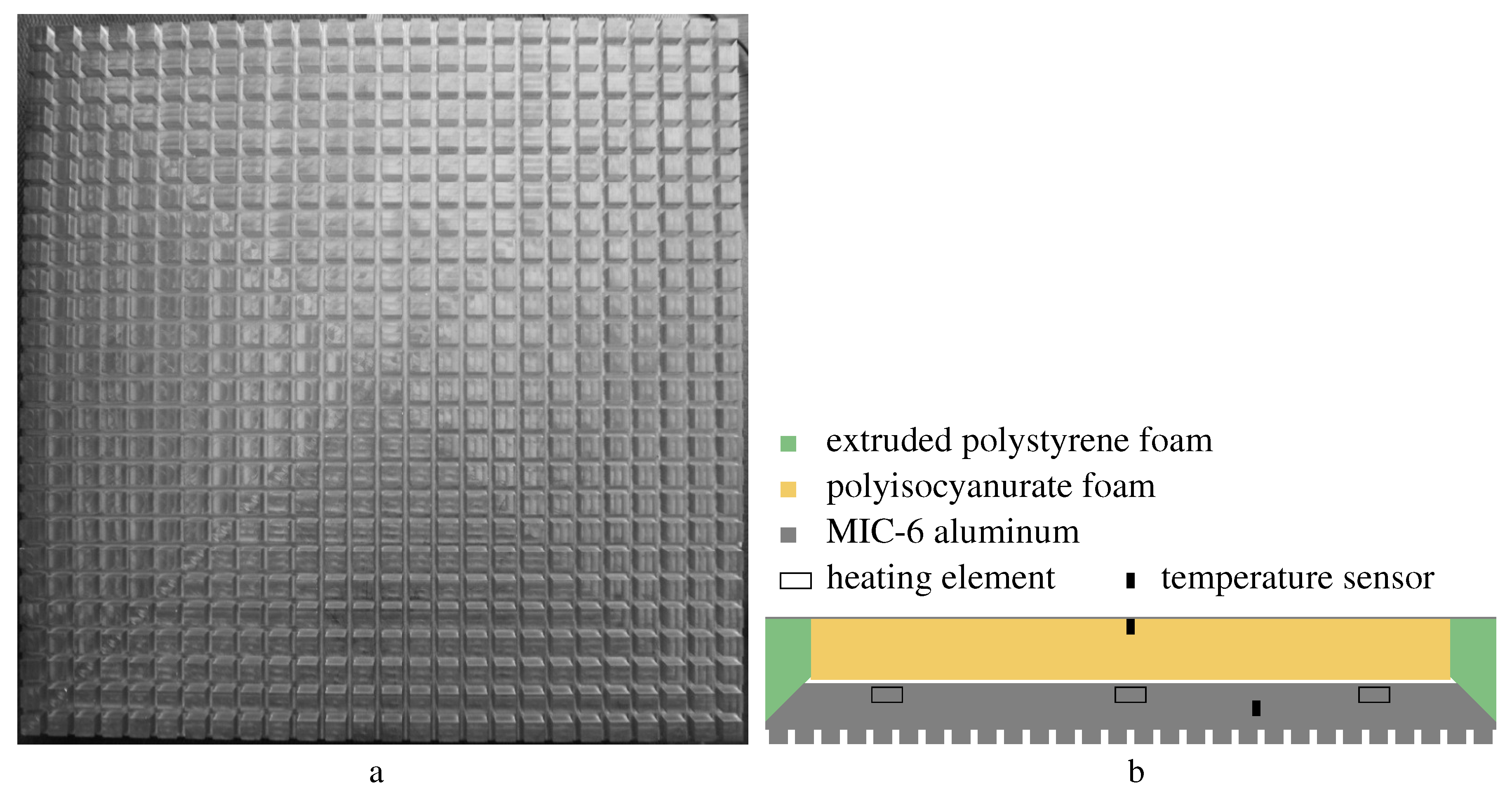
Appendix A.1. The Plate
Figure A1a shows the rough surface of the test plate; it was milled from a slab of MIC-6 aluminum (Al) to have (676 of) square posts spaced on 11.7 mm centers over the plate. The area of the top of each post was , which was 50.4% of its cell. The RMS height-of-roughness . Openness . Embedded in the plate are 9 electronic resistors as heating elements and a Texas Instruments LM35 Precision Centigrade Temperature Sensor. 2.54 cm of thermal insulating foam separates the back of the plate from a 0.32 mm thick sheet of aluminum with an LM35 temperature sensor at its center. Figure A1b is a cross-section illustration of the plate assembly.
Figure A2.
(a) plate in wind-tunnel; (b) wind-tunnel boundary layers.
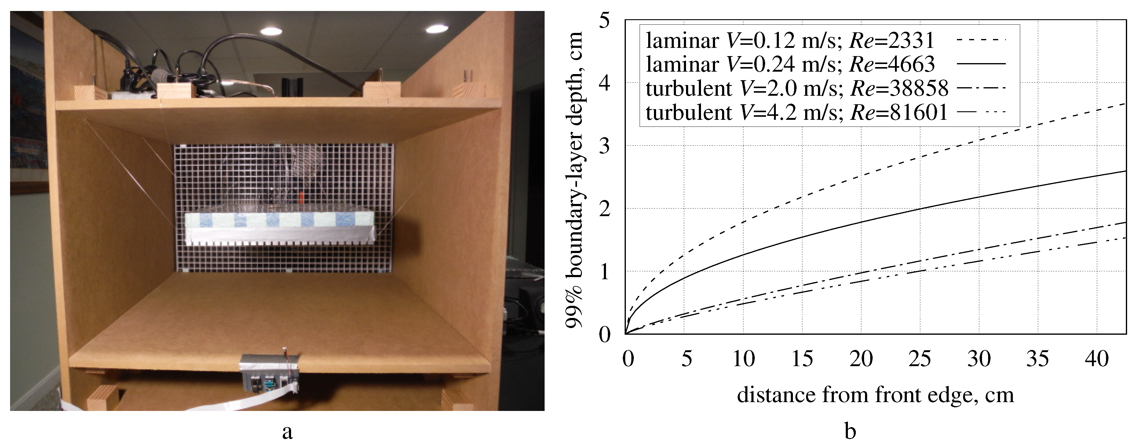
Appendix A.2. Wind Tunnel
The fan pulls air from the test chamber’s open intake through the test chamber. The fan blows directly into a diffuser made of folded plastic mesh to disrupt vortexes generated by the fan. In a sufficiently large room, the disrupted vortexes dissipate before being drawn into the open intake.
To guarantee isobaric (no pressure drop) flow, the wind-tunnel must be sufficiently large that its test chamber and plate assembly boundary layers do not interact at fan-capable airspeeds.
The wind-tunnel test chamber in Figure A2a has a cross-section and a 61 cm depth. This allows the plate assembly to be centered in the wind-tunnel with 15 cm of space on all sides. The fan pulling air through the test chamber produces a maximum airspeed of 4.65 m/s ( along the 30.5 cm square plate). Its minimum nonzero airspeed is 0.12 m/s ().
Test chamber laminar and turbulent 99% boundary layer thicknesses (Schlichting [7]) are:
Figure A2b shows that the 15 cm clearance between the plate and the test chamber walls is sufficient to prevent their boundary layers from interacting at airspeeds within the fan’s capabilities.
The plate assembly is suspended from six lengths of 0.38 mm-diameter steel piano wire terminated at twelve zither tuning pins in wooden blocks fastened to the exterior of the test chamber. The plate is suspended face-down to minimize the natural convection from the test-surface. With the plate assembly in the test chamber, the airspeed increases in proportion to the reduction of test chamber aperture by the plate’s cross-sectional area :
Appendix A.3. Automation
Data capture and control of convection experiments are performed by an “STM32F3 Discovery 32-Bit ARM M4 72MHz” development board. The program written for the STM32F3 captures readings and writes them to the microprocessor’s non-volatile RAM, controls the plate heating, servos the fan speed, and later uploads its data to a computer through a USB cable.
Once per second during an experiment, the program calibrates and reads each on-chip 12 bit analog-to-digital converter 16 times, summing the sixteen 12 bit readings to create a 16 bit reading per converter.
Rotations of the fan are sensed when a fan blade interrupts an infrared beam. The microprocessor controls a solid-state relay (supplying power to the fan) to maintain a fan rotation rate, , which is dialed into switches. At r/min, the microprocessor pulses power to the fan to phase-lock the beam interruption signal to an internal clock. At r/min, the microprocessor servos the duty cycle of a 7.5 Hz square-wave gating power to the fan. This system operates at .
Figure A3.
(a) Airspeed versus fan speed; (b) Fan PLL variability.
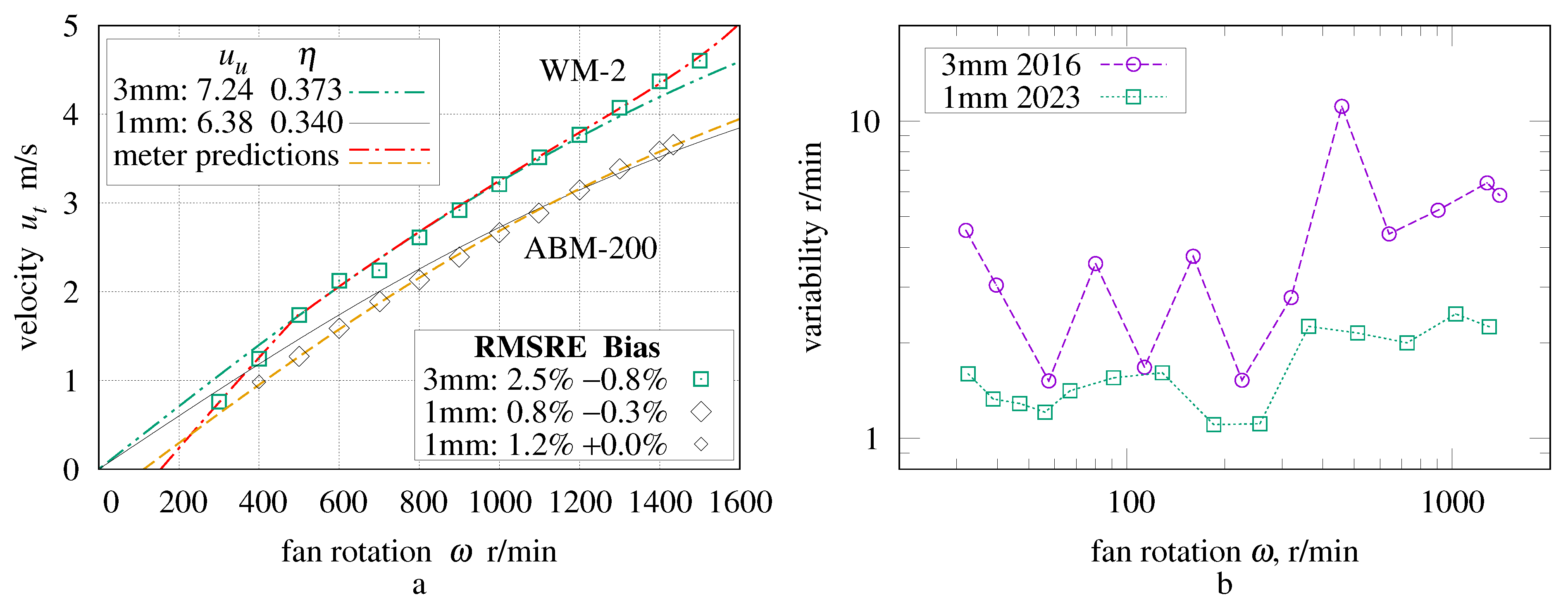
Appendix A.4. Calibration
The correspondence between fan rotation rate and test chamber airspeed u was determined using an “Ambient Weather WM-2”, which specifies an accuracy of of reading. After 2017 an “ABM-200 Airflow & Environmental Meter” specifying an accuracy of of reading between 2.2 m/s and 62.5 m/s, was used.
The “UtiliTech 20 inch 3-Speed High Velocity Floor Fan” has three blades with maximum radius m. Its characteristic length is its hydraulic-diameter, m. The velocity of the blade tips is , where is the number of rotations per minute. The Reynolds number of the fan is:
The 3 blade tips trace the whole circumference in only 1/3 of a rotation, hence the 3 in the denominator.
Faster fan rotation yields diminishing increases of test-chamber airspeed , suggesting Formula (A4), where is the limiting velocity for arbitrarily fast rotation, and coefficient converts fan to test-chamber . Figure A3a gives the parameters and measurements at . The “3 mm” points are the WM-2 measurements of the 3 mm plate in the original wind-tunnel; The “1 mm” points are the ABM-200 measurements of the 1 mm plate in the tunnel with a new diffuser and fan cowling.
Airspeeds slower than 2 m/s should be nearly proportional to . Both anemometers show evidence of dry (bearing) friction in Figure A3a. The ABM-200 “meter predictions” trace plots ; the WM-2 “meter predictions” trace plots when and otherwise. A mistake in the 2016 measurement software under-counted fan rotations at r/min. This is compensated by replacing in Formulas (A3) and (A4) with in the WM-2 “meter predictions”. The RMSRE and Bias are relative to the “meter predictions”. The second “1 mm” row includes the point at 400 r/min.
Figure A3b shows the fan speed variability for each downward-facing experiment; these are used by the measurement uncertainty calculations. The differences reflect improvements in the fan-control software written by the author (28 September 2023).
Figure A4.
Ambient sensors.
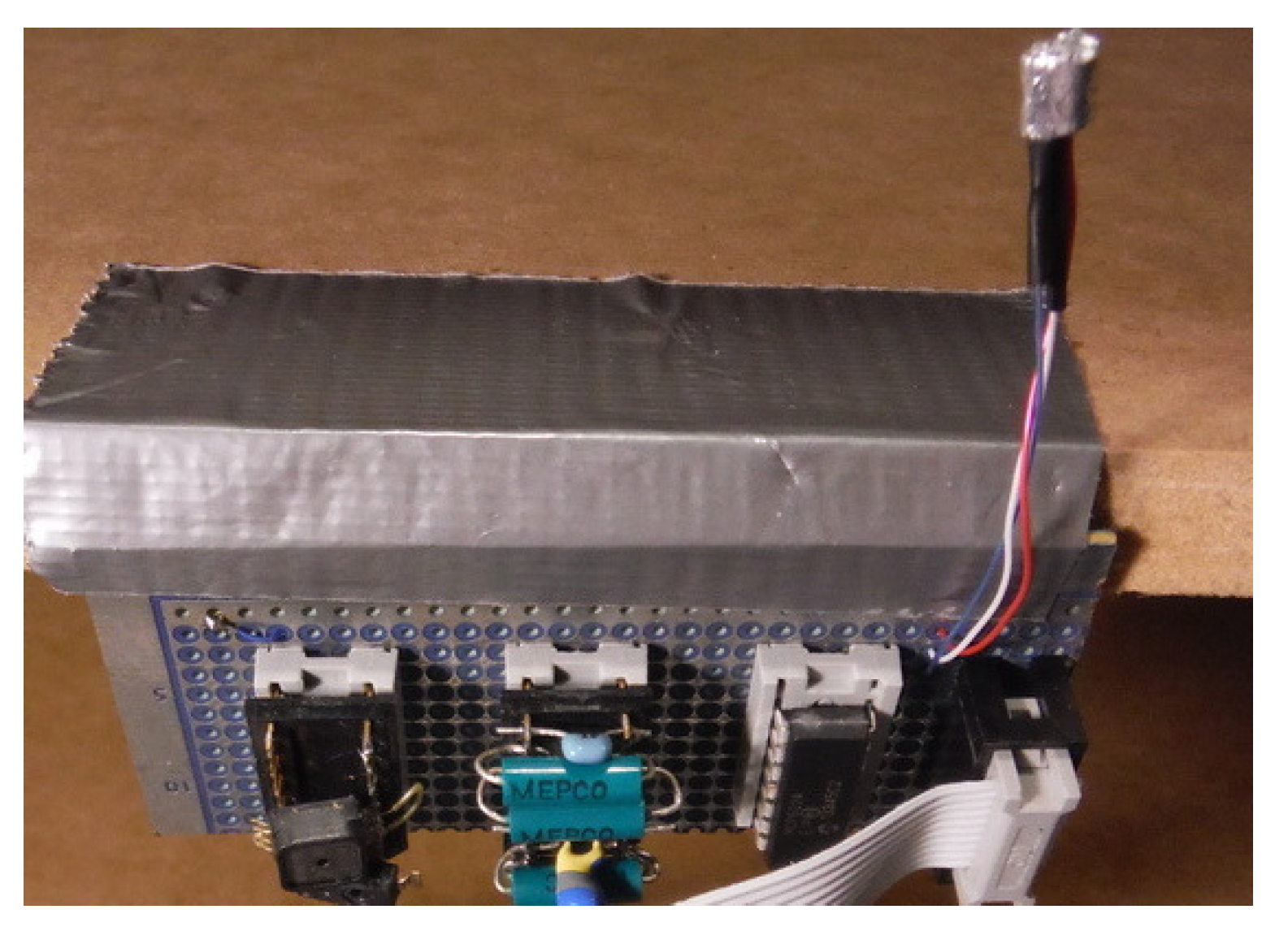
Appendix A.5. Ambient Sensing
Figure A4 shows the ambient sensor board which was at the lower edge of the test chamber in Figure A2a. It measures the pressure, relative humidity (RH), and air temperature at the wind-tunnel intake. Wrapped in aluminum tape to minimize radiative heat transfer, the LM35 temperature sensor projects into the tunnel. To minimize self-heating, the LM35 is powered only while being sampled.
Table A1.
Physical parameters.
Appendix A.6. Physical Parameters
Table A1 lists the static parameters from measurements and specifications.
The effective may differ from the medium-density-fiberboard emissivity given by Rice [42] because the temperatures of the test chamber surfaces may not be uniform. Through the open intake, the plate also exchanges thermal radiation with objects in the room having different temperatures.
Appendix A.7. Modeling of Parasitic Heat Flows
At low airflow velocities, the sides of the insulation behind the test plate can leak more heat than the test-surface transfers, shrinking to 6% at 1300 r/min. To compensate, expected side heat transfers will be subtracted from the (combined) measured heat flow.
Figure A2a shows duck tape applied to the lower 54% of the plate’s side, which corresponds to 50% coverage of the XPS foam wedge. For this partial tape coverage, Formula (A5) is the area proportional mean of the duck tape emissivity and XPS emissivity. Barreira, Almeida, and Simões [43] measured emissivities of 0.86 and 0.89 from two brands of “duck tape”; the larger value is used for the aged tape on the plate sides. As of this writing, published emissivity measurements of XPS foam have not been located.
Relative to the theory in Jaffer [28], natural convection measurements () from the plate assembly over the span of inclinations have less than 2.8% RMSRE when calculated with ; the RMSRE increases to either side of 0.515. This value is consistent with natural convection measurements of the plate assembly without tape.
Figure A5.
XPS wedge conduction.
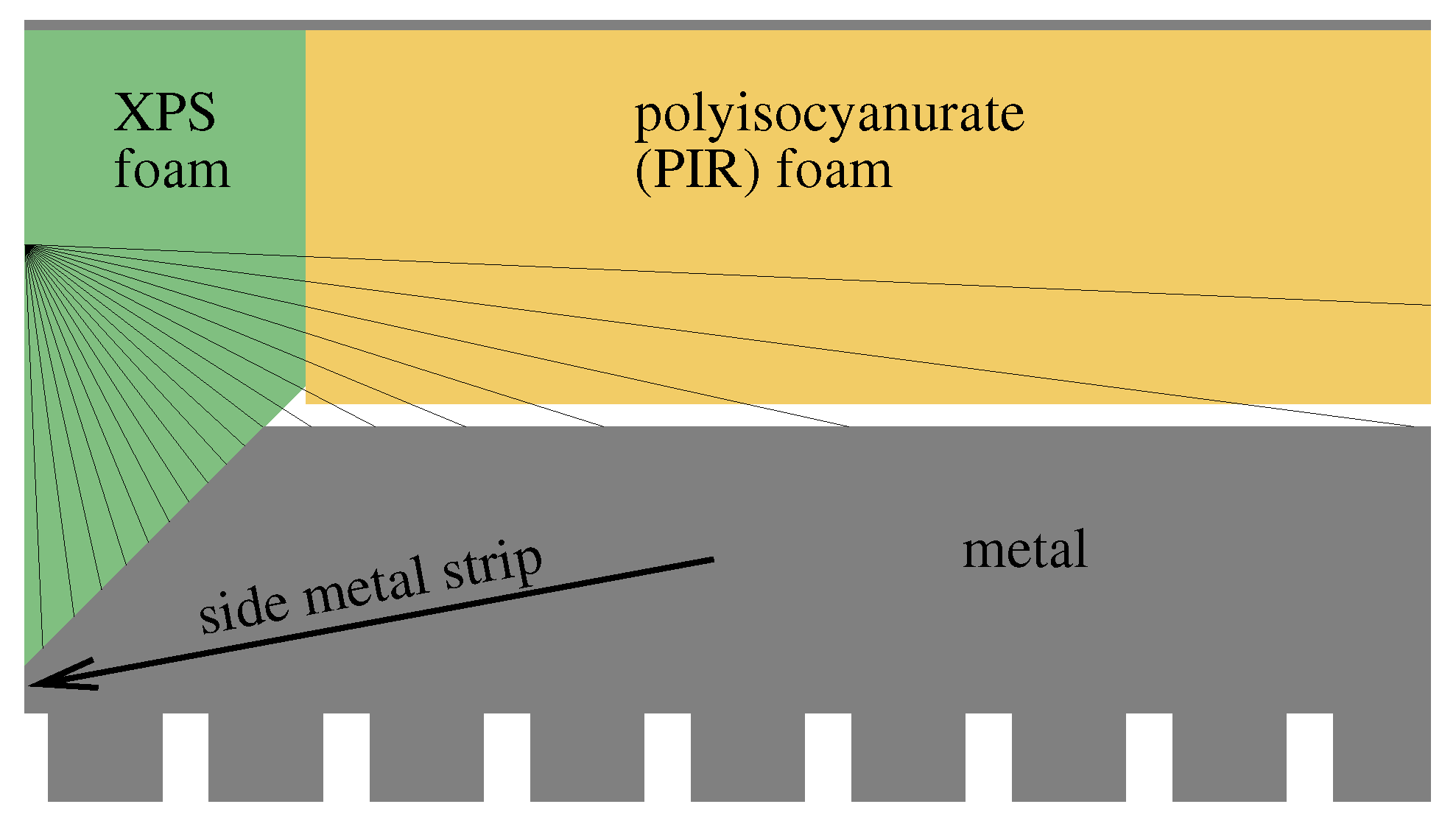
The four sides are not isothermal; a 3.5 mm metal strip (see cross-section Figure A5) runs the length of the side; and a -tall wedge of extruded polystyrene foam (XPS) insulation fills the metal slab’s chamfer. The local surface conductance at elevation z (from the wedge point) is found by averaging the reciprocal distance to slab metal with respect to angle :
Forced air flows parallel to the long dimension on two sides, but flows into the windward side and away from the leeward side. Air heated by the windward side reduces heat transfer from the test-surface; air heated by the test-surface suppresses heat transfer from the leeward side. Hence, the model excludes windward and leeward forced convection. The total forced convective conductance of the flow-parallel foam wedges is calculated by integrating in series (reciprocal of the sum of reciprocals, which is also the -norm) with the local surface conductance , where is the pierced-laminar convection calculated by applying the transform (57) to the pierced-laminar convection Formula (92):
The natural convection flow from the vertical faces is upward, perpendicular to the horizontal forced flow; hence, the forced convection and the natural convective conductance combine as the -norm (introduced in Section 13). The resulting mixed convective conductance is in mild competition with the side radiative conductance, ; they combine as the -norm:
Each of the four side’s natural convective conductance is vertical plate Formula (A9) from Jaffer [28], with characteristic length , where the metal slab thickness .
Appendix A.8. Measurement Methodology
The measurement methodology employed is unusual. Instead of waiting until the plate reaches thermal equilibrium, the plate is heated to 15 K above ambient, heating stops, the fan runs at the designated speed, and convection cools the plate. All of the sensor readings are captured each second during the 102 minute process, Table A2 lists the dynamic physical quantities measured each second. Table A3 lists computed quantities. Both and are subtracted from the combined heat flow. The mean of over the time interval in which drops by half (or exceeds 6142 s total time) is the result from that experiment.
Table A2.
Dynamic quantities.
Table A3.
Computed quantities.
Appendix A.9. Heat Balance
Collecting into Formula (A10) those terms which have a factor of temperature difference , Formula (A11) is the heat balance equation of the plate during convective cooling:
The plate and ambient temperatures are functions of time t. Determined experimentally during heating, the temperature group-delay through the 2.54 cm block of insulation between the slab and back sheet is 110 s:
Appendix A.10. Measurement Uncertainty
Following Abernethy, Benedict, and Dowdell [44], the final steps in processing an experiment’s data are:
- Using Equation (A14), calculate the sensitivities of convected power per each parameter’s average over the measurement time-interval;
- Multiply the absolute value of each sensitivity by its estimated parameter bias to yield component uncertainties;
- Calculate combined bias uncertainty as the root-sum-squared (RSS) of the component uncertainties;
- Calculate the RSS combined measurement uncertainty as the RSS of the combined bias uncertainty and twice the product of the rotation rate sensitivity and variability.
Table A4 and Table A5 list the sensitivity, bias, and uncertainty for each component contributing more than 0.20% uncertainty for the 3 mm and 1 mm roughness plates, respectively. Figure A6a and Figure A6b show the measurements relative to the present theory for rough flow and turbulent flow, respectively.
Table A4.
Estimated measurement uncertainties, bi-level 3 mm roughness at 59,593.
Table A5.
Estimated measurement uncertainties, bi-level 1 mm roughness at .
Figure A6.
(a) Measured versus theory mm; (b) Measured versus theory mm.
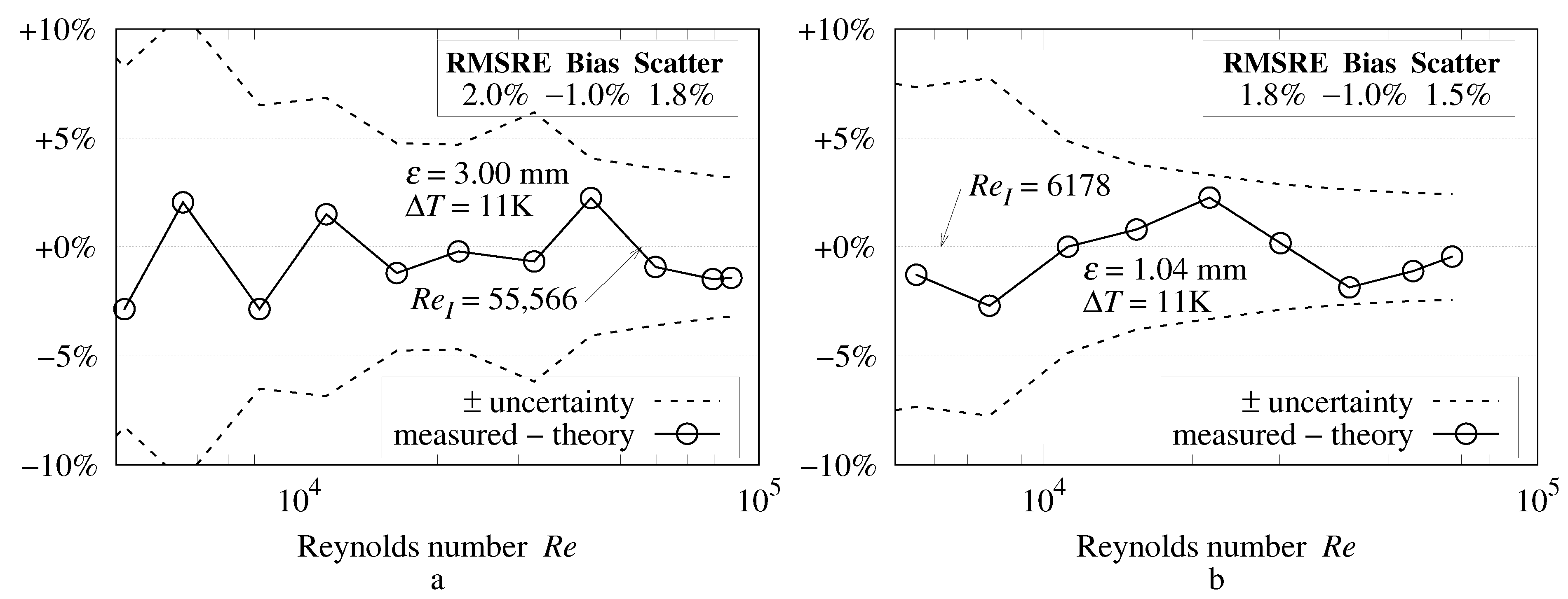
Appendix A.11. Details
Documentation, photographs, electrical schematics, and software source-code for the apparatus, as well as calibration and measurement data, are available from [accessed on 6 December 2023]: http://people.csail.mit.edu/jaffer/convect.
Appendix B. Thermal and Transport Properties of Humid Air
Wexler [37] approximates the (partial) pressure of saturated water vapor as:
where T is absolute temperature in Kelvins.
An ideal gas has density , where the gas constant . Air with relative humidity , modeled as a mixture of dry air and water vapor, has density:
where the molar masses of air and water are kg/mol and kg/mol.
Tsilingiris [38] approximates the specific heats of dry air and water vapor:
Morvay and Gvozdenac [39] approximate the viscosity of air and water vapor as:
where . They combine these into dynamic viscosity using absolute humidity , the mass ratio of water vapor to air.
Morvay and Gvozdenac [39] approximate the thermal conductivity of water vapor at :
Kadoya, Matsunaga, and Nagashima [36] approximate the thermal conductivity of dry air as:
where
Both Morvay and Gvozdenac [39] and Tsilingiris [38] develop the combined thermal conductivity k as:
References
- Prandtl, L. Zur turbulenten Stromüng in Rohren und längs Platten. Ergebnisse Der Aerodynamische Versuchsanst Zu Göttingen 1932, 4, 18–29. [Google Scholar]
- von Kármán, T. Theorie des Reibungswiderstandes [Theory of the frictional resistance]. In Proceedings of the Hydromechanische Probleme des Schiffsantriebs, Hamburg, Germany, 18–19 May 1932; pp. 50–73. [Google Scholar] [CrossRef] [Scilit]
- Prandtl, L.; Schlichting, H. The Resistance Law for Rough Plates; Translation; Navy Department, the David W. Taylor Model Basin: Bethesda, MD, USA, 1934. [Google Scholar]
- Nikuradse, J. Laws of Flow in Rough Pipes; VDI-Verl: Berlin, Germany, 1933; p. 361. [Google Scholar]
- Schlichting, H. Experimental Investigation of the Problem of Surface Roughness; Technical Report TM 823; NACA: Washington, DC, USA, 1937. [Google Scholar]
- Hama, F.R. Boundary layer characteristics for smooth and rough surfaces. Trans. Soc. Nav. Arch. Marine Engrs. 1954, 62, 333–358. [Google Scholar]
- Schlichting, H. Boundary Layer Theory, 7th ed.; Kestin, J., Translator; McGraw Hill: New Delhi, India, 2014. [Google Scholar]
- Pimenta, M.M.; Moffat, R.J.; Kays, W.M. The Turbulent Boundary Layer: An Experimental Study of the Transport of Momentum and Heat with the Effect of Roughness; Department of Mechanical Engineering, Stanford University: Stanford, CA, USA, 1975. [Google Scholar]
- Mills, A.F.; Hang, X. On the Skin Friction Coefficient for a Fully Rough Flat Plate. J. Fluids Eng. 1983, 105, 364–365. [Google Scholar] [CrossRef] [Scilit]
- White, F. Viscous Fluid Flow, 3rd ed.; McGraw-Hill: New York, NY, USA, 2006. [Google Scholar]
- Churchill, S.W. Theoretically based expressions in closed form for the local and mean coefficients of skin friction in fully turbulent flow along smooth and rough plates. Int. J. Heat Fluid Flow 1993, 14, 231–239. [Google Scholar] [CrossRef] [Scilit]
- Colebrook, C.F. Turbulent Flow in Pipes, with Particular Reference to the Transition Region Between the Smooth and Rough Pipe Laws. J. Inst. Civ. Eng. 1939, 11, 133–156. [Google Scholar] [CrossRef] [Scilit]
- Bergstrom, D.J.; Akinlade, O.G.; Tachie, M.F. Skin Friction Correlation for Smooth and Rough Wall Turbulent Boundary Layers. J. Fluids Eng. 2005, 127, 1146–1153. [Google Scholar] [CrossRef] [Scilit]
- Jiménez, J. Turbulent Flows Over Rough Walls. Annu. Rev. Fluid Mech. 2004, 36, 173–196. [Google Scholar] [CrossRef] [Scilit]
- Chung, D.; Hutchins, N.; Schultz, M.P.; Flack, K.A. Predicting the Drag of Rough Surfaces. Annu. Rev. Fluid Mech. 2021, 53, 439–471. [Google Scholar] [CrossRef] [Scilit]
- Lienhard, J.H., IV; Lienhard, V.J.H. A Heat Transfer Textbook, 5th ed.; Version 5.10; Phlogiston Press: Cambridge, MA, USA, 2020. [Google Scholar]
- Incropera, F.; DeWitt, D.; Bergman, T.; Lavine, A. Fundamentals of Heat and Mass Transfer; Wiley: Hoboken, NJ, USA, 2007. [Google Scholar]
- Žukauskas, A.; Šlančiauskas, A. Heat Transfer in Turbulent Fluid Flows; Hemisphere Publishing Corp: Washington, DC, USA, 1987. [Google Scholar]
- Schubauer, G.B.; Skramstad, H.K. Laminar-Boundary-Layer Oscillations and Transition on a Flat Plate; Technical Report NACA-TR-909; NASA: Washington, DC, USA, 1948. [Google Scholar]
- Gebers, F. Ein Beitrag zur experimentellen Ermittlung des Wasserwiderstandes gegen bewegte Köper. Schiffbau 1908, 9, 435–452, 475–485. [Google Scholar]
- Gebers, F. Das Ähnlichkeitsgesetz für den Flächenwiderstand in Wasser geradling fortbewegter polierter Platten. Schiffbau 1920, 22, 687–930. [Google Scholar]
- Smith, D.W.; Walker, J.D. Skin Friction Measurements in Incompressible Flow; Technical Report R-26; NASA: Washington, DC, USA, 1959. [Google Scholar]
- Spalding, D.B.; Chi, S.W. The drag of a compressible turbulent boundary layer on a smooth flat plate with and without heat transfer. J. Fluid Mech. 1964, 18, 117–143. [Google Scholar] [CrossRef] [Scilit]
- Kestin, J.; Maeder, P.; Wang, H. Influence of turbulence on the transfer of heat from plates with and without a pressure gradient. Int. J. Heat Mass Transf. 1961, 3, 133–154. [Google Scholar] [CrossRef] [Scilit]
- Reynolds, W.C.; Kays, W.M.; Kline, S.J. Heat Transfer in the Turbulent Incompressible Boundary Layer, Part 4—Effect of Location of Transition and Prediction of Heat Transfer in a Known Transition Region; Technical Report NASA-MEMO-12-4-58W; NASA: Washington, DC, USA, 1958. [Google Scholar]
- Afzal, N.; Seena, A.; Bushra, A. Turbulent flow in a machine honed rough pipe for large Reynolds numbers: General roughness scaling laws. J. Hydro-Environ. Res. 2013, 7, 81–90. [Google Scholar] [CrossRef] [Scilit]
- Flack, K.A.; Schultz, M.P.; Barros, J.M.; Kim, Y.C. Skin-friction behavior in the transitionally-rough regime. Int. J. Heat Fluid Flow 2016, 61, 21–30. [Google Scholar] [CrossRef] [Scilit]
- Jaffer, A. Natural Convection Heat Transfer from an Isothermal Plate. Thermo 2023, 3, 148–175. [Google Scholar] [CrossRef] [Scilit]
- Lienhard, J.H.V. Heat Transfer in Flat-Plate Boundary Layers: A Correlation for Laminar, Transitional, and Turbulent Flow. J. Heat Transf. 2020, 142, 061805. [Google Scholar] [CrossRef] [Scilit]
- Colburn, A.P. A method of correlating forced convection heat-transfer data and a comparison with fluid friction. Int. J. Heat Mass Transf. 1964, 7, 1359–1384. [Google Scholar] [CrossRef] [Scilit]
- Goldstein, R.; Sparrow, E.; Jones, D. Natural convection mass transfer adjacent to horizontal plates. Int. J. Heat Mass Transf. 1973, 16, 1025–1035. [Google Scholar] [CrossRef] [Scilit]
- Lloyd, J.; Moran, W. Natural convection adjacent to horizontal surface of various planforms. J. Heat Transf. 1974, 96, 443–447. [Google Scholar] [CrossRef] [Scilit]
- Churchill, S.W.; Usagi, R. A general expression for the correlation of rates of transfer and other phenomena. AIChE J. 1972, 18, 1121–1128. [Google Scholar] [CrossRef] [Scilit]
- Tuck, E.O.; Kouzoubov, A. A laminar roughness boundary condition. J. Fluid Mech. 1995, 300, 59–70. [Google Scholar] [CrossRef] [Scilit]
- Kiefer, J. Sequential Minimax Search for a Maximum. Proc. Am. Math. Soc. 1953, 4, 502–506. [Google Scholar] [CrossRef]
- Kadoya, K.; Matsunaga, N.; Nagashima, A. Viscosity and Thermal Conductivity of Dry Air in the Gaseous Phase. J. Phys. Chem. Ref. Data 1985, 14, 947–970. [Google Scholar] [CrossRef] [Scilit]
- Wexler, A. Vapor Pressure Formulation for Water in Range 0 to 100 °C. A Revision. J. Res. Natl. Bur. Stand. 1976, 80A, 775–785. [Google Scholar] [CrossRef] [Scilit] [PubMed]
- Tsilingiris, P. Thermophysical and transport properties of humid air at temperature range between 0 and 100 °C. Energy Convers. Manag. 2008, 49, 1098–1110. [Google Scholar] [CrossRef] [Scilit]
- Morvay, Z.K.; Gvozdenac, D.D. Toolbox 6: Thermodynamic and Transport Properties of Moist Air. In Applied Industrial Energy and Environmental Management Part III: Fundamentals for Analysis and Calculation of Energy and Environmental Performance; John Wiley & Sons, Ltd.: Hoboken, NJ, USA, 2016. [Google Scholar]
- Pramuditya, S. Water Thermodynamic Properties; Technical report; Bandung Institute of Technology: Bandung, Indonesia, 2011. [Google Scholar]
- Wagner, W.; Pruß, A. The IAPWS Formulation 1995 for the Thermodynamic Properties of Ordinary Water Substance for General and Scientific Use. J. Phys. Chem. Ref. Data 2002, 31, 387–535. [Google Scholar] [CrossRef] [Scilit]
- Rice, R. Emittance factors for infrared thermometers used for wood products. Wood Fiber Sci. 2004, 36, 520–526. [Google Scholar]
- Barreira, E.; Almeida, R.M.S.F.; Simões, M.L. Emissivity of Building Materials for Infrared Measurements. Sensors 2021, 21, 1961. [Google Scholar] [CrossRef] [Scilit]
- Abernethy, R.; Benedict, R.; Dowdell, R. ASME Measurement Uncertainty. ASME J. Fluids Eng. 1985, 107, 161–164. [Google Scholar] [CrossRef] [Scilit]
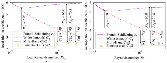
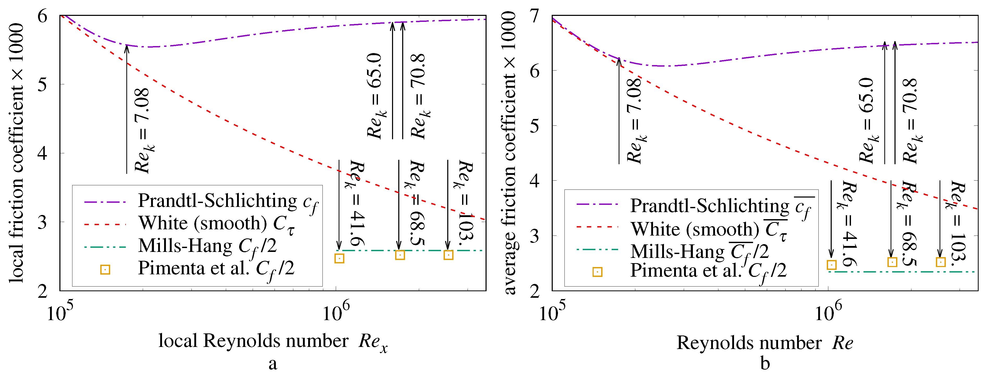
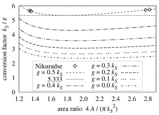
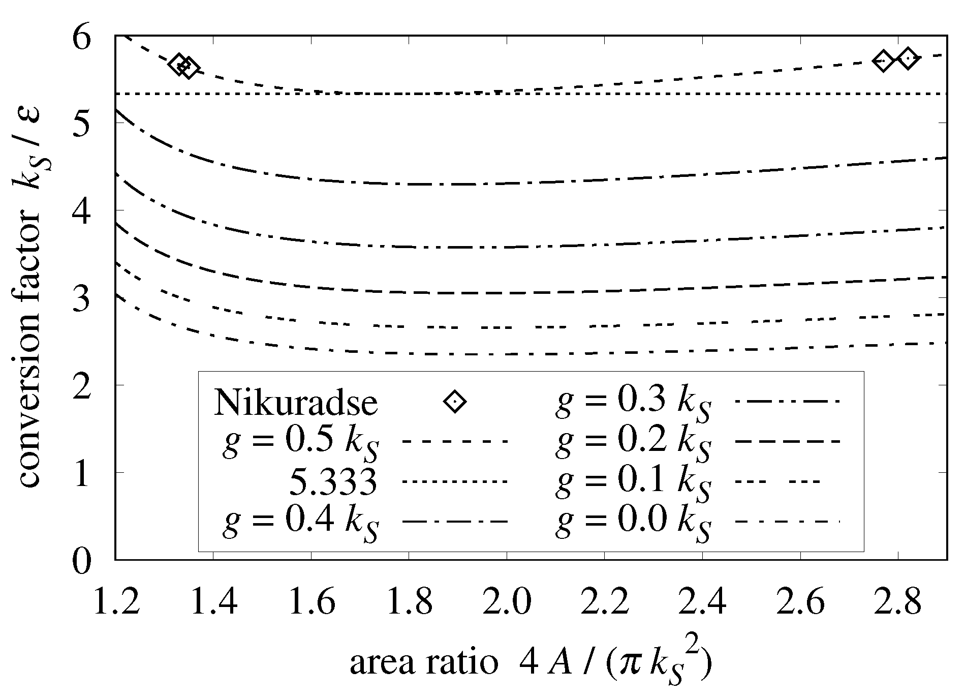
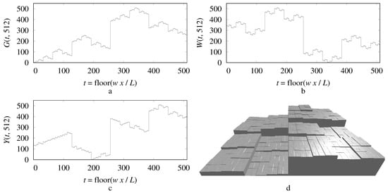
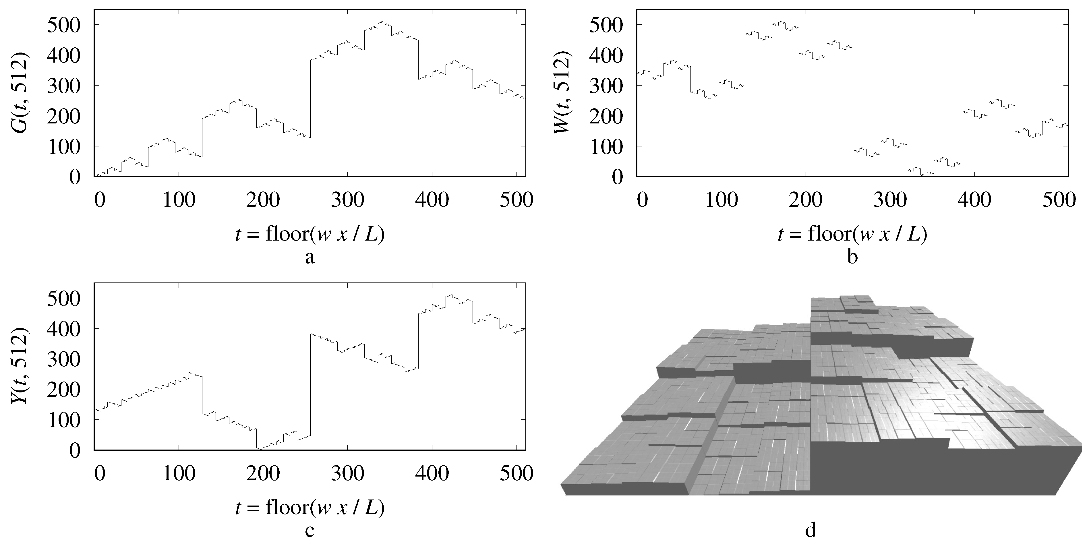
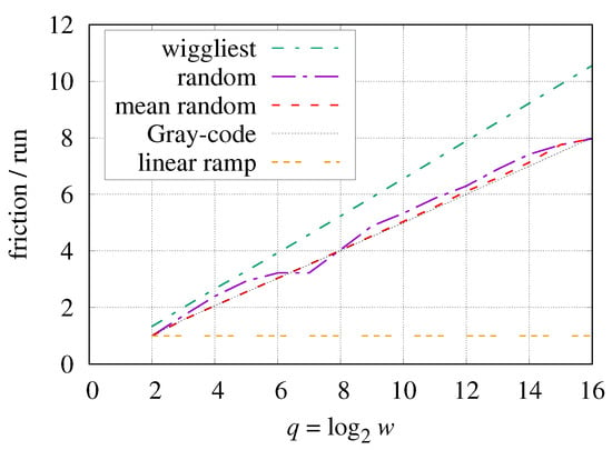
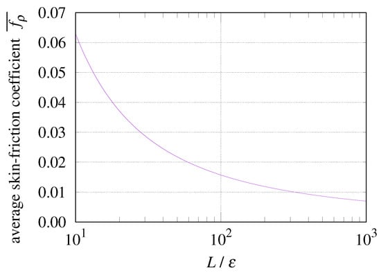
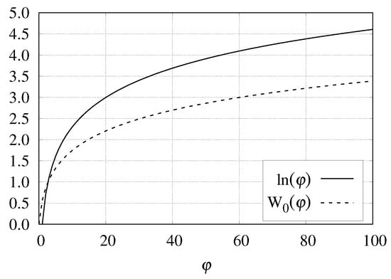
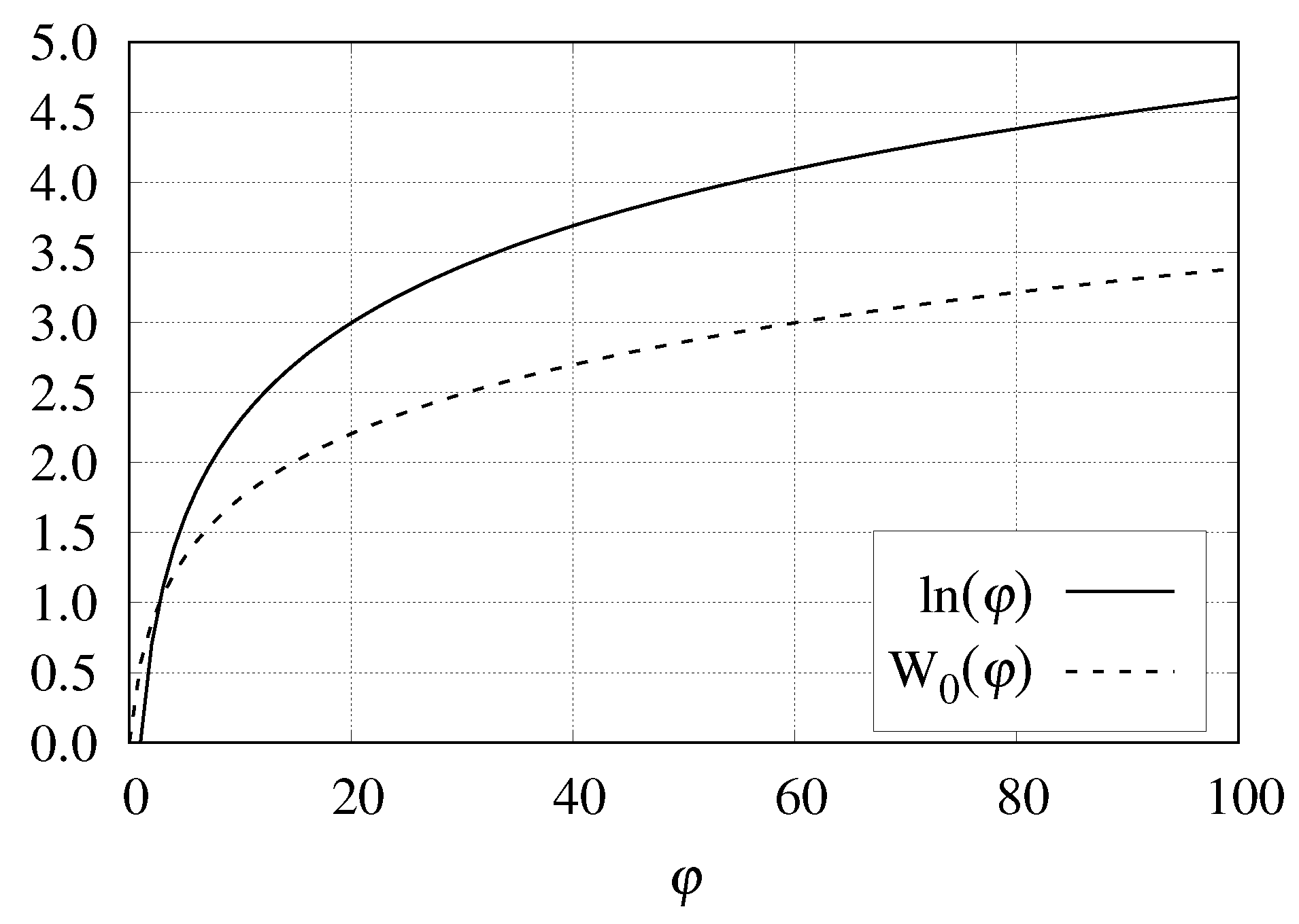
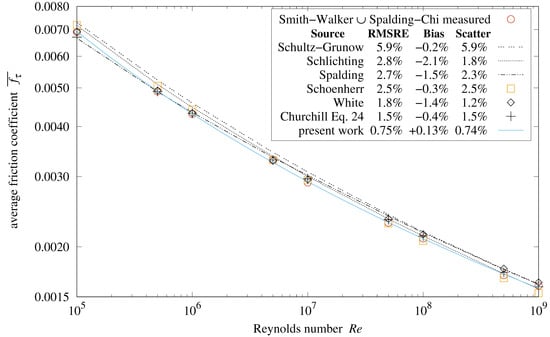
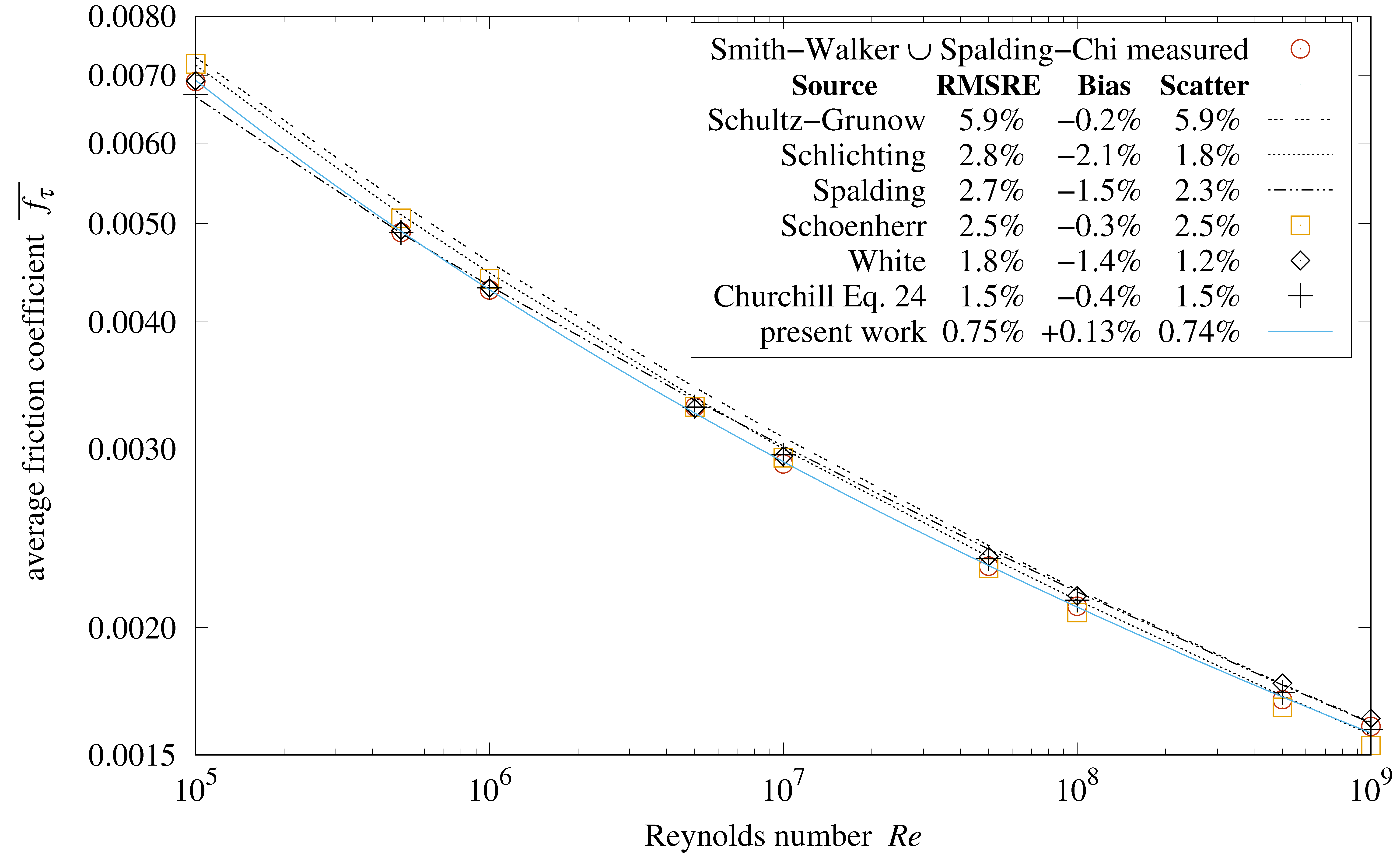
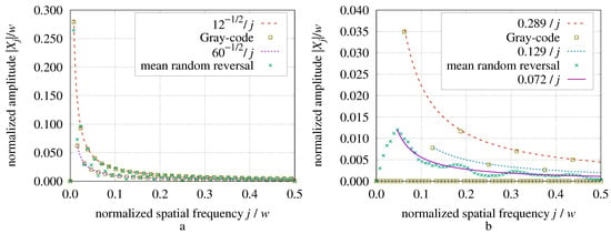
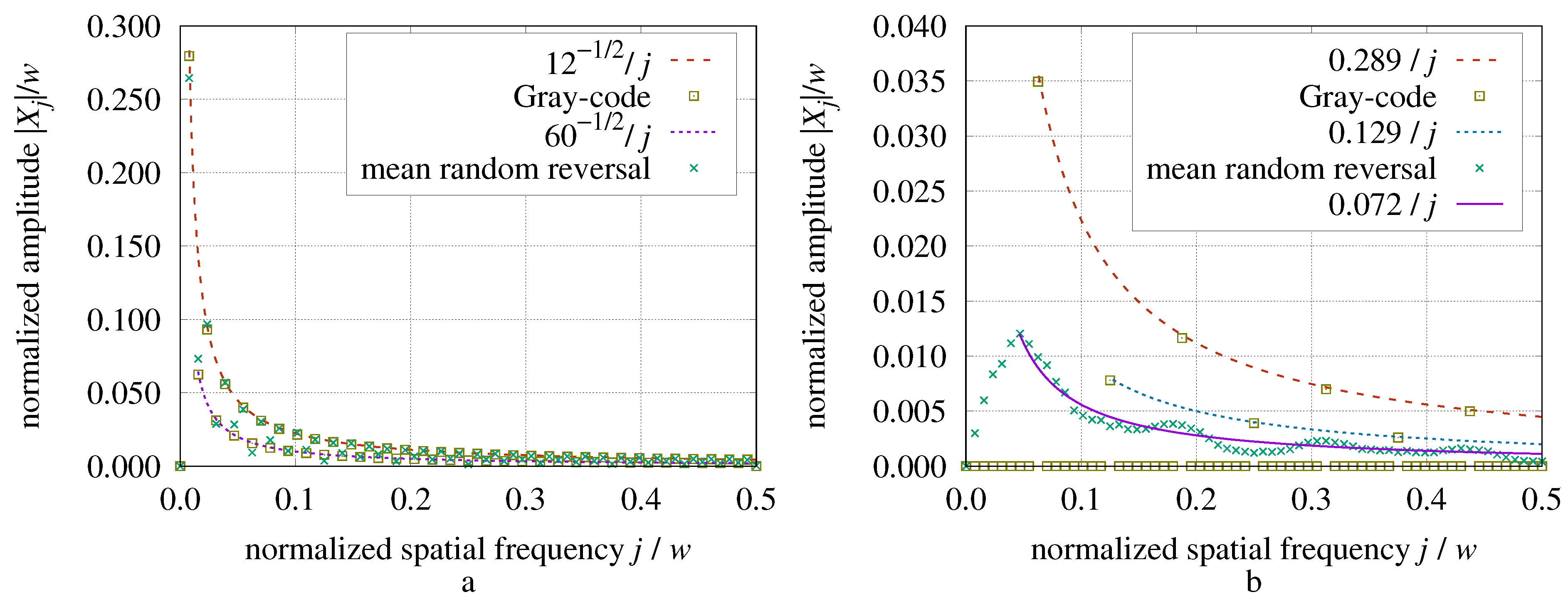
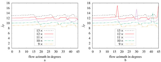
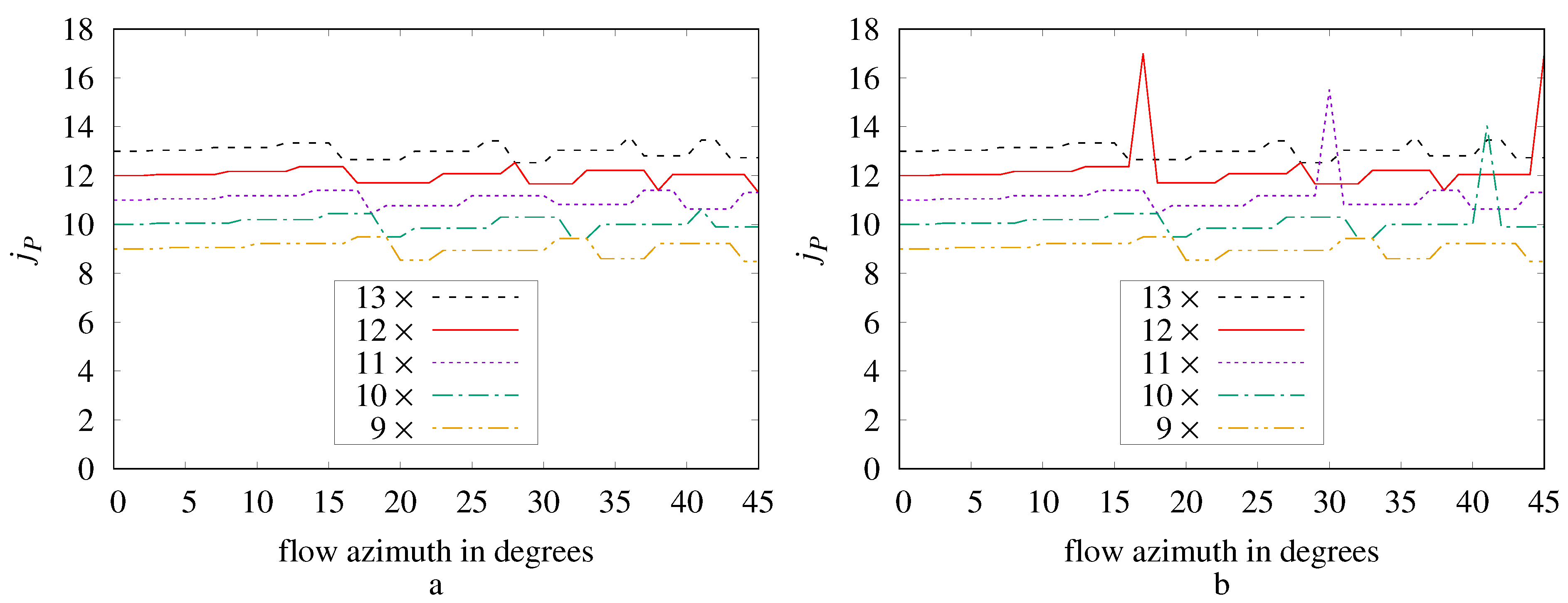
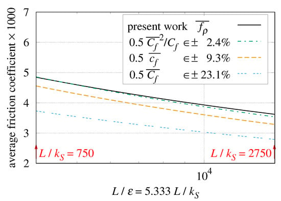
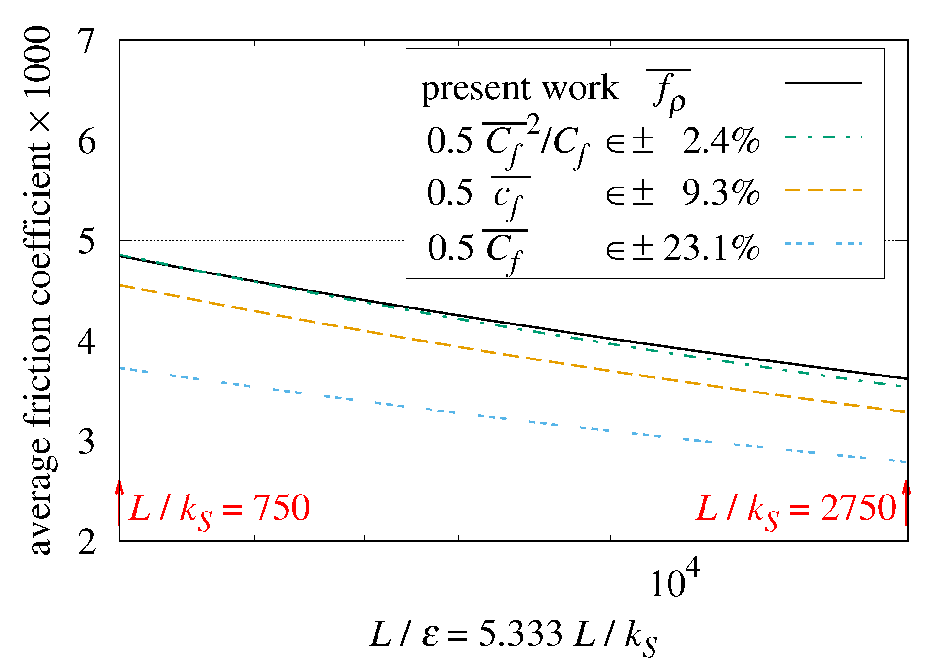
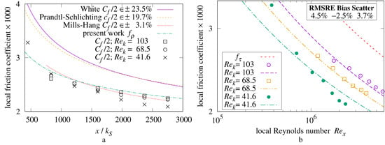
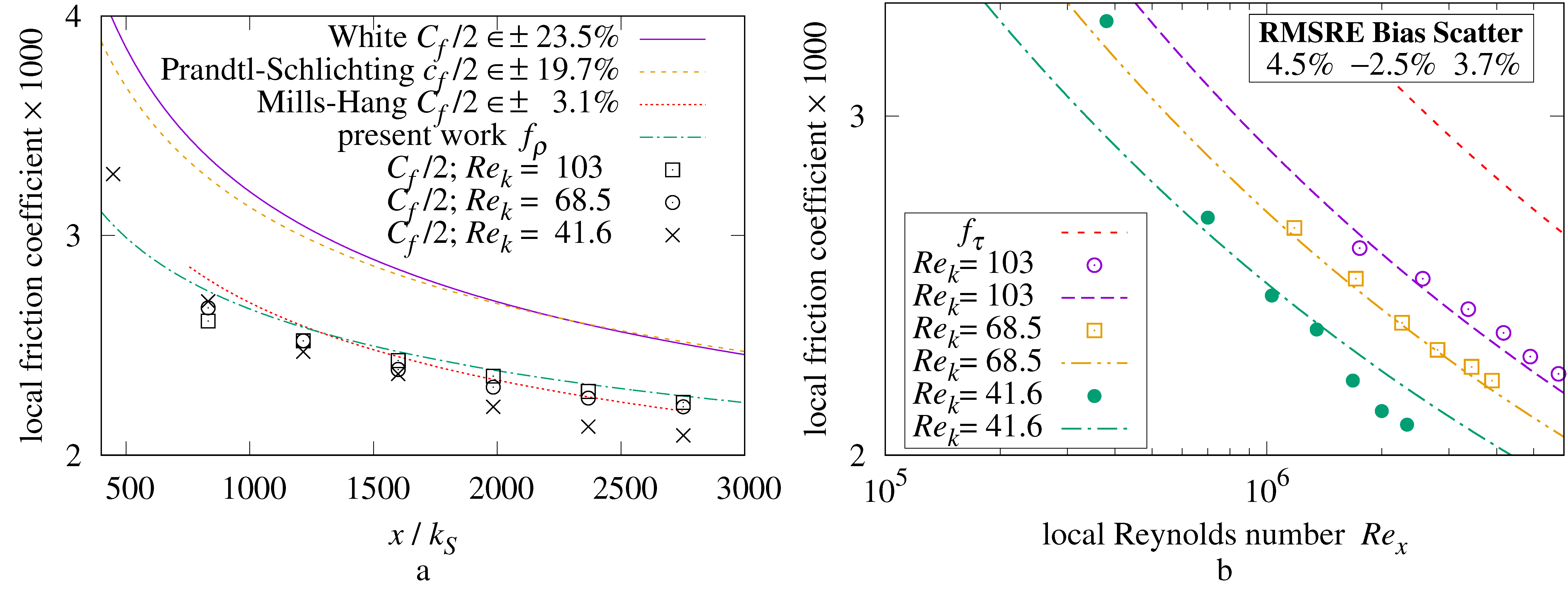
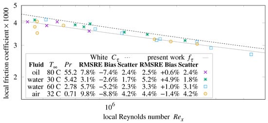
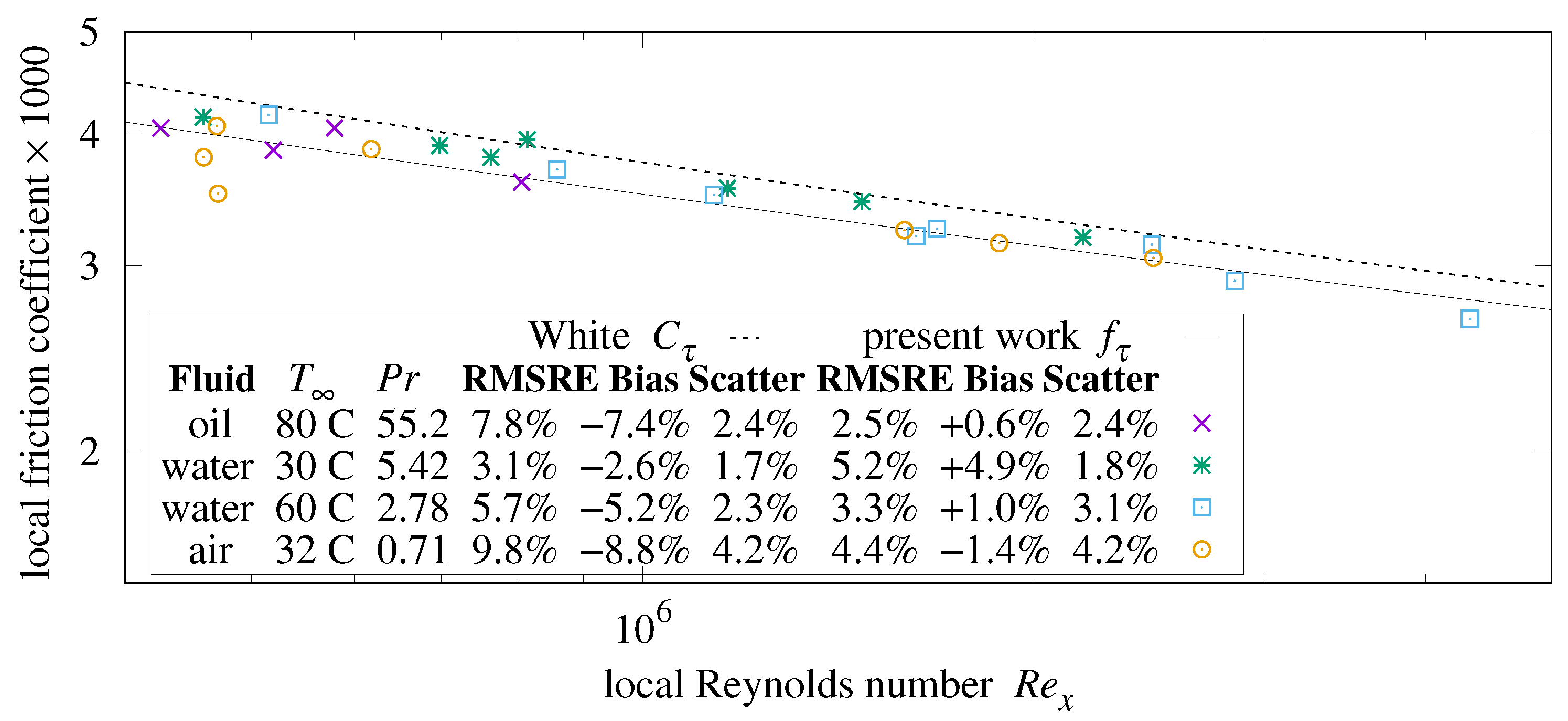
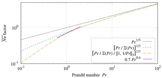
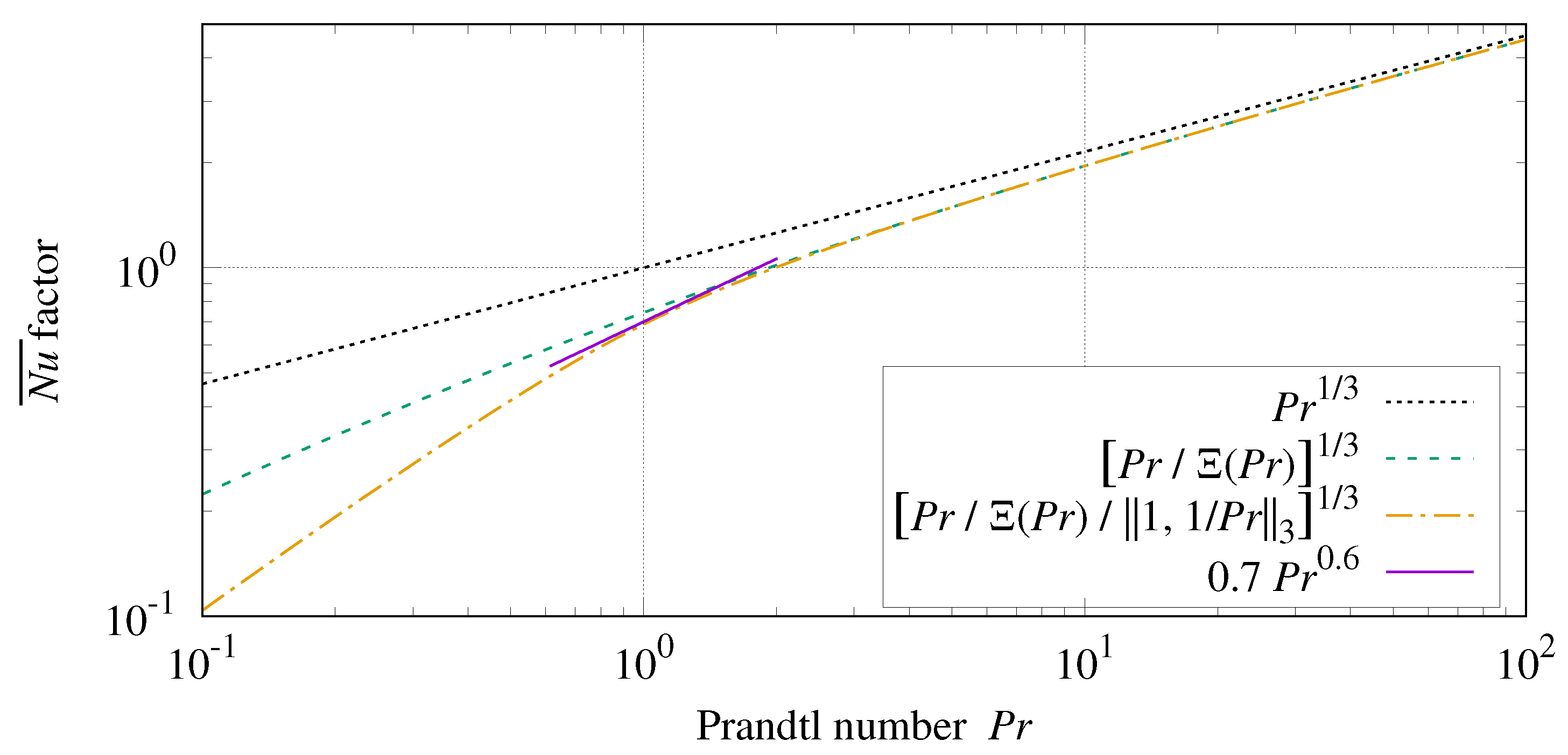
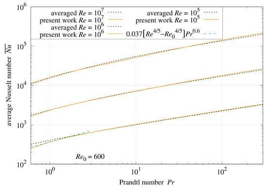
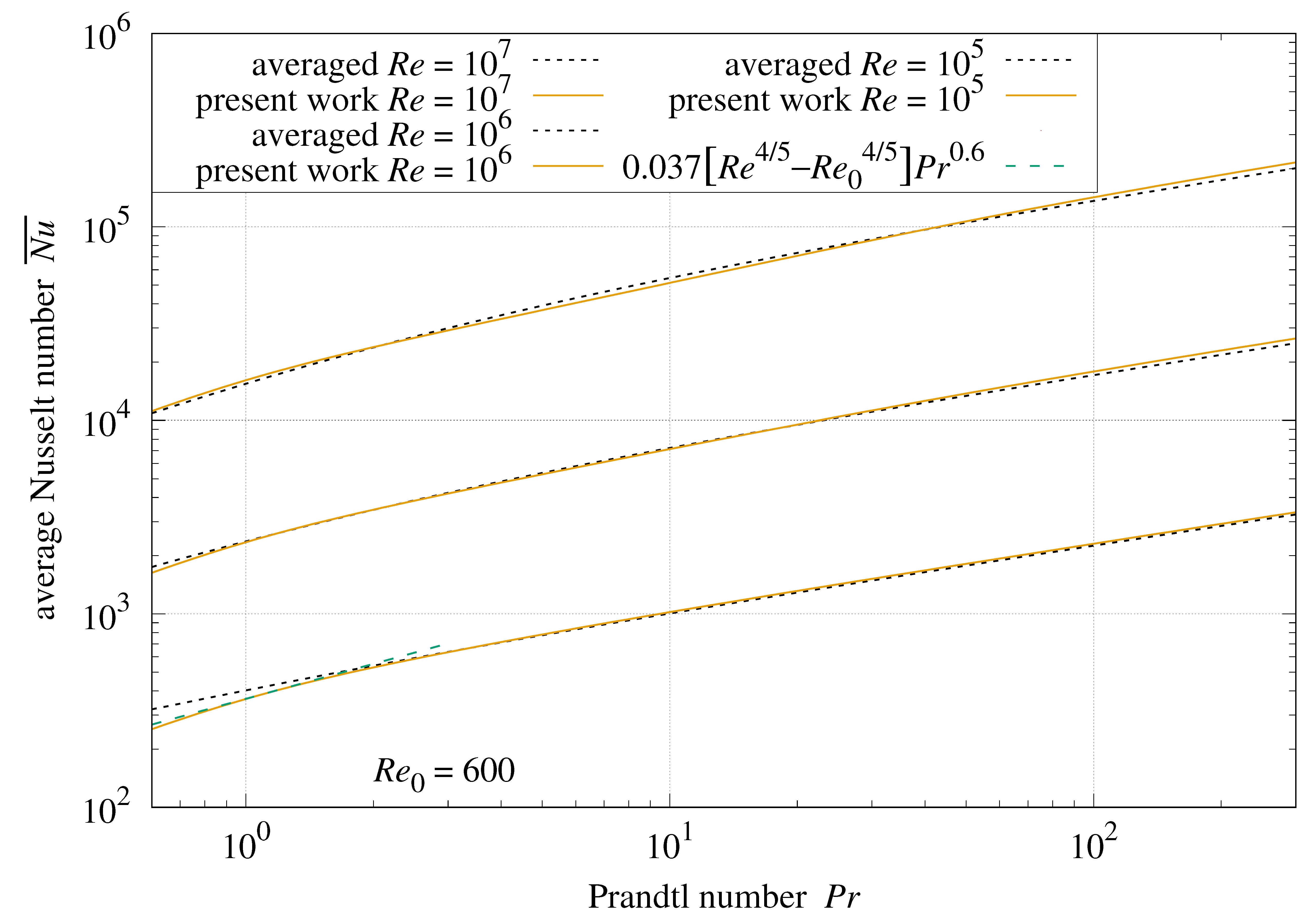
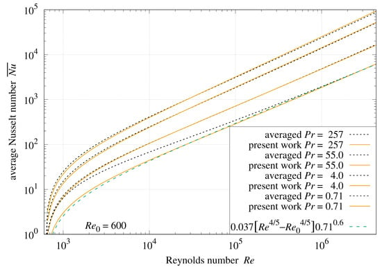
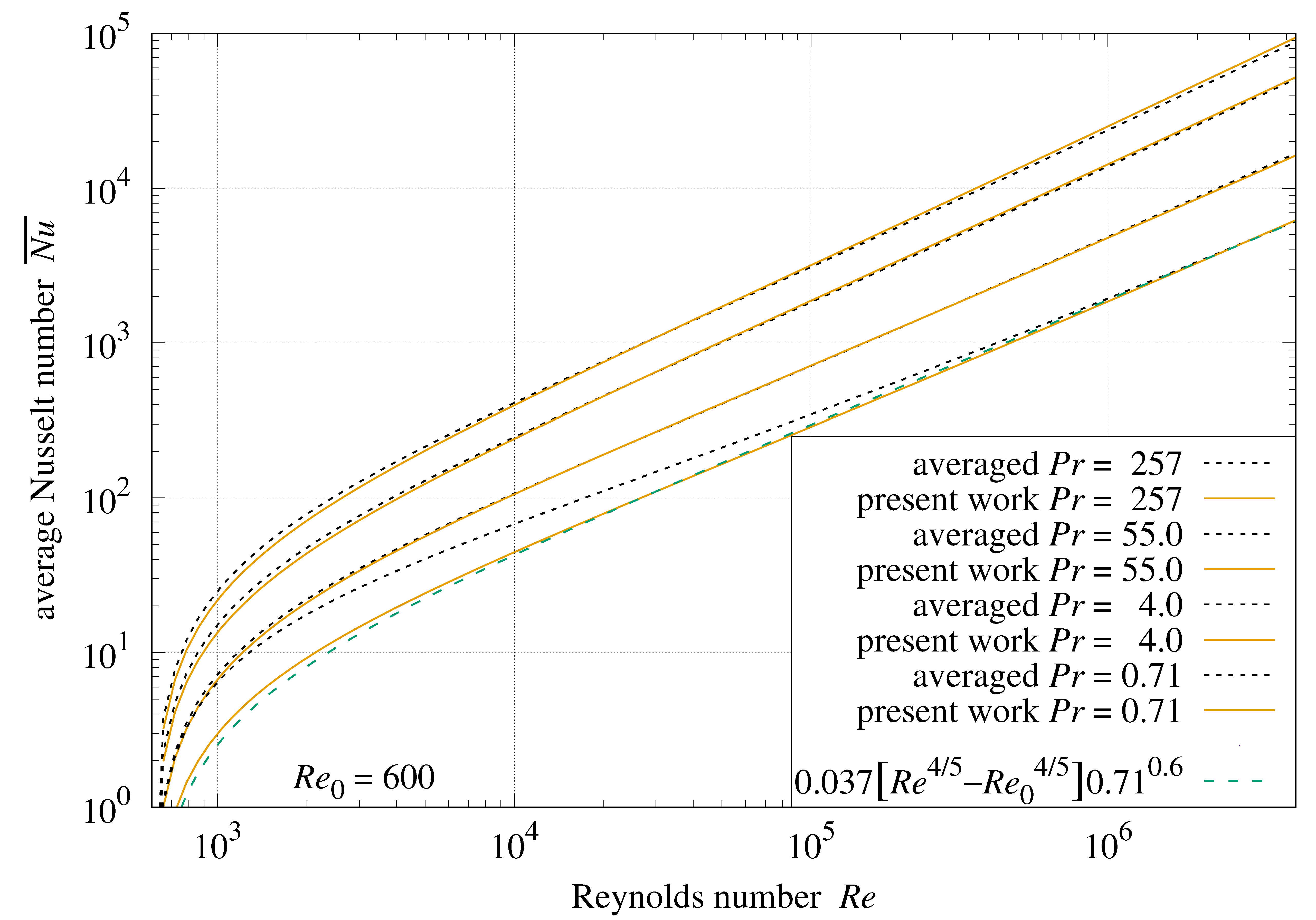
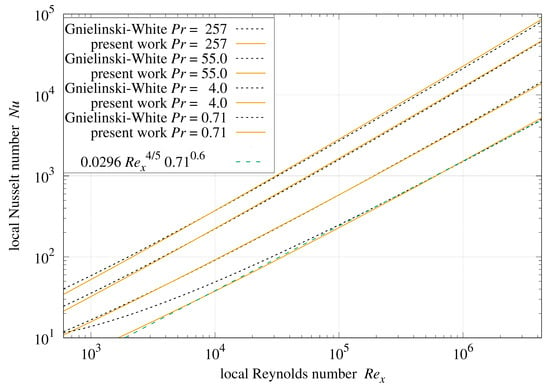
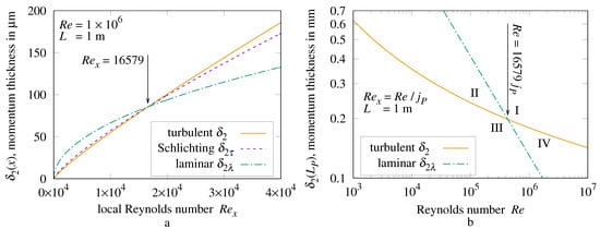
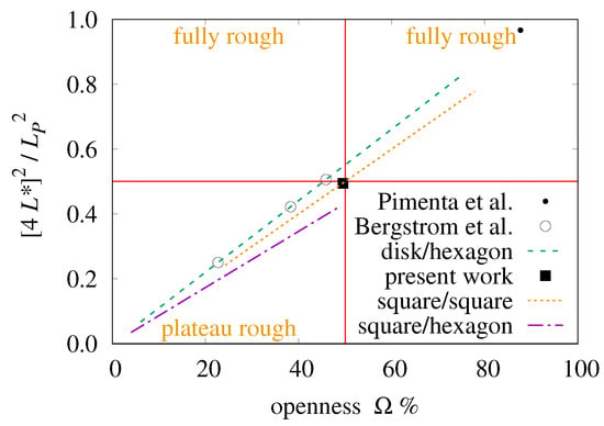
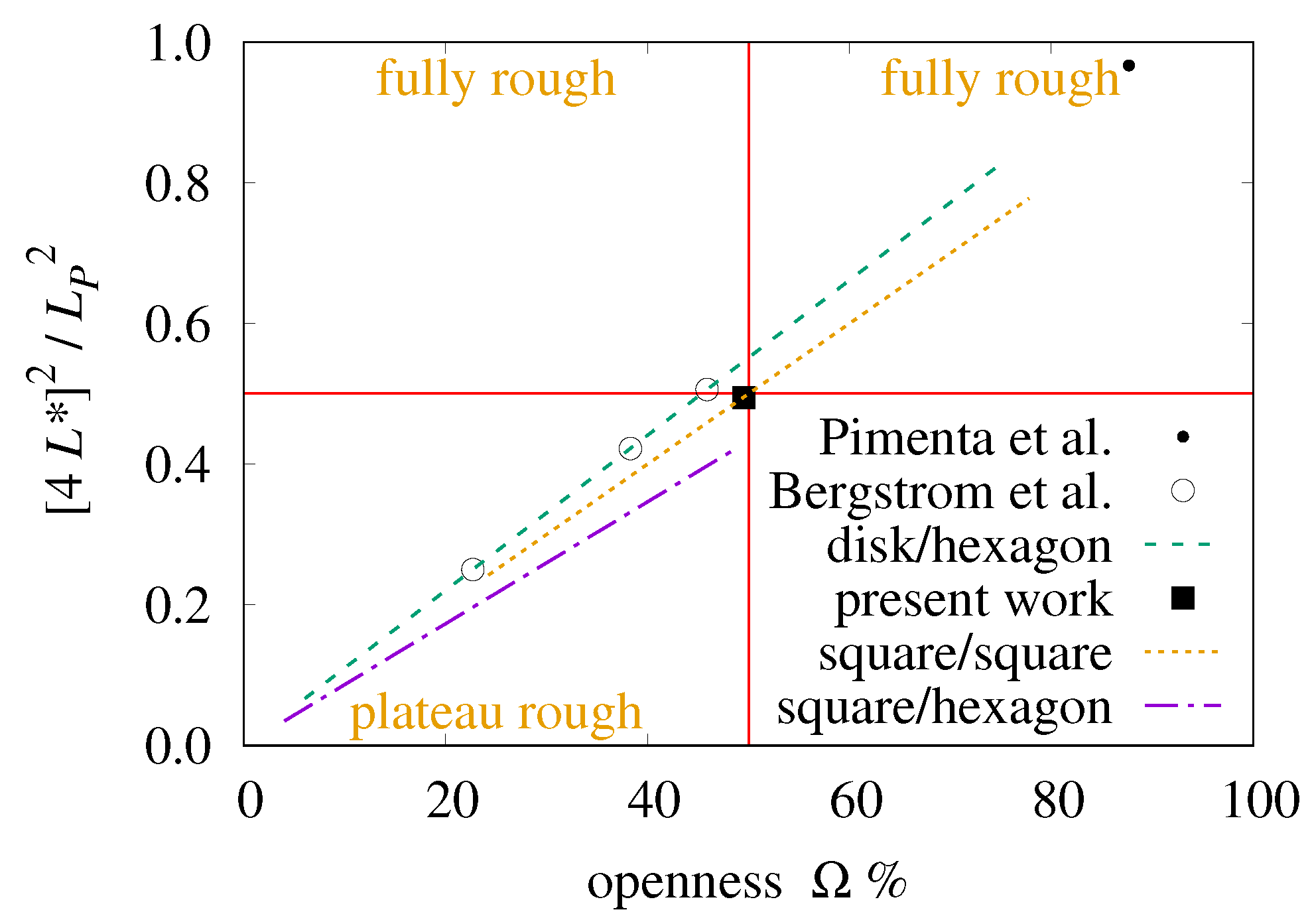
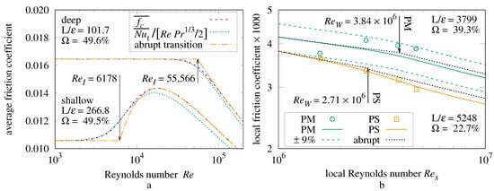
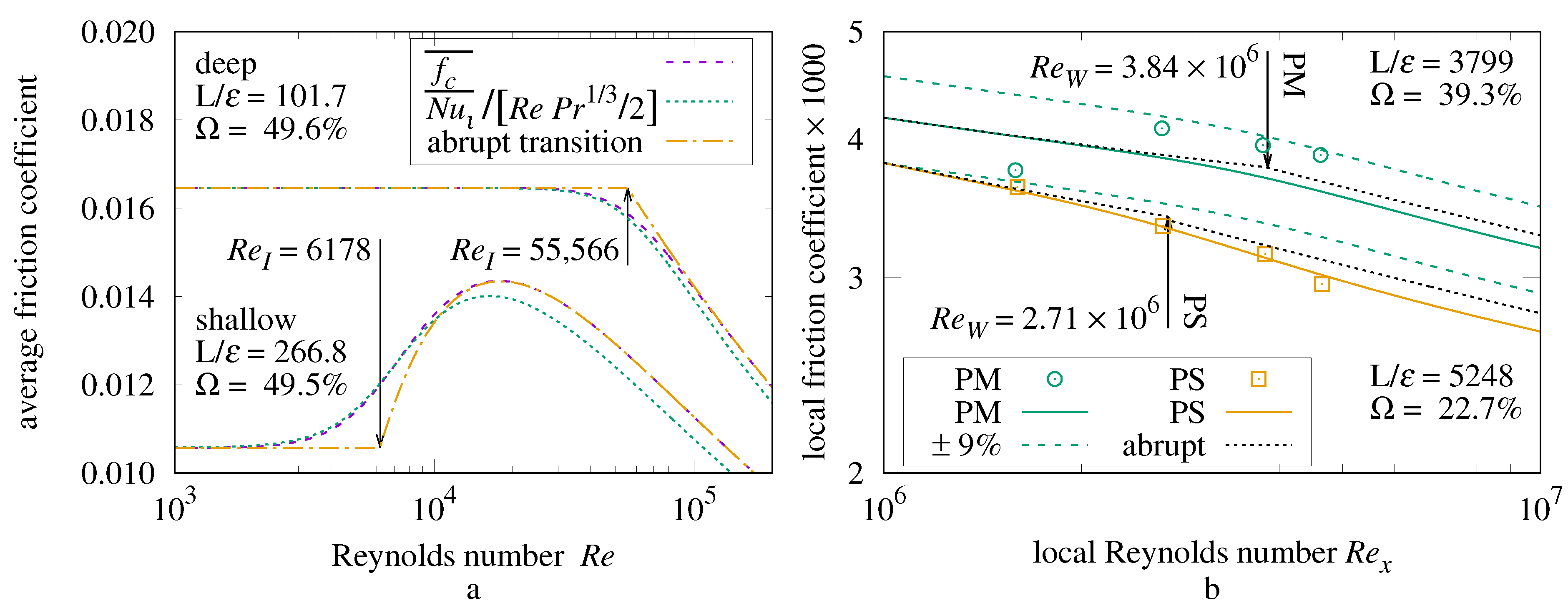
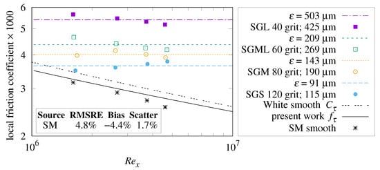
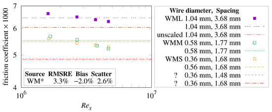
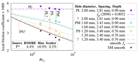
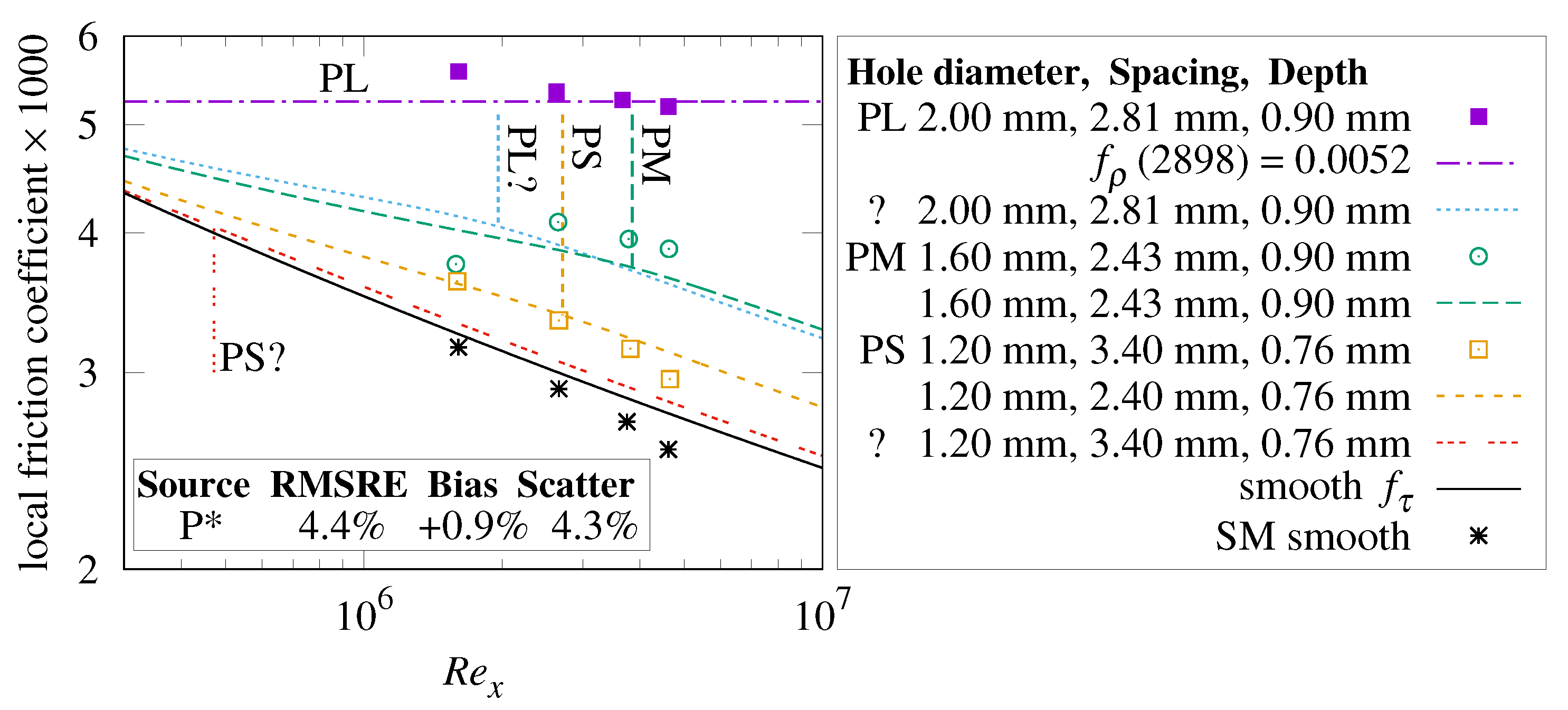
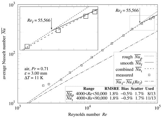
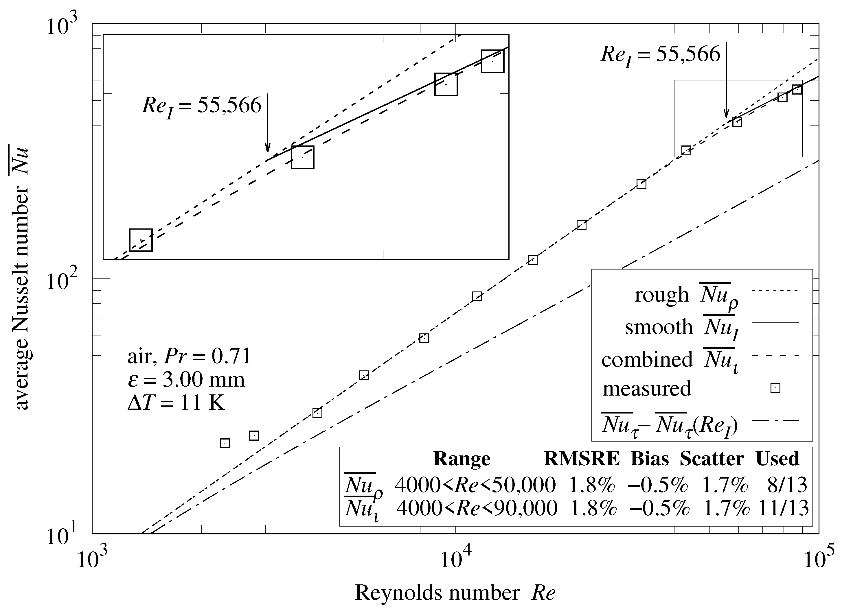
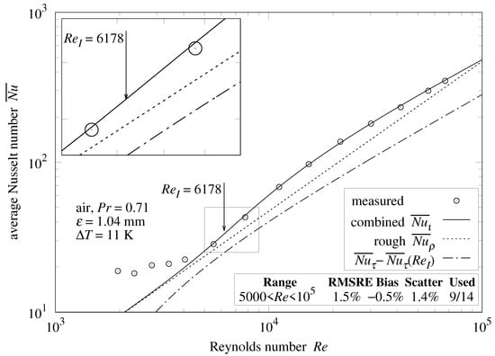
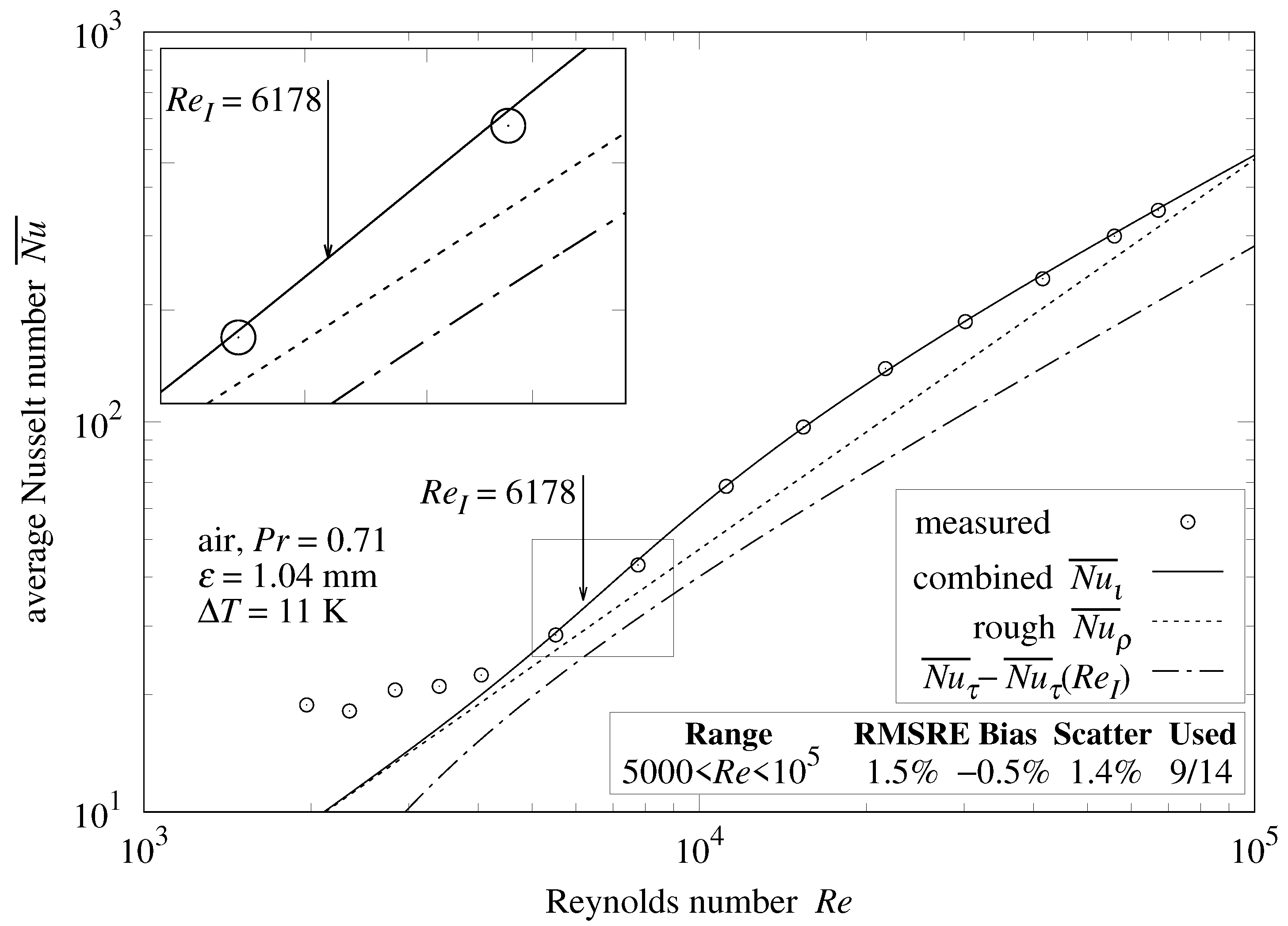
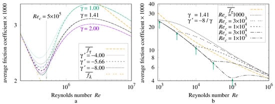
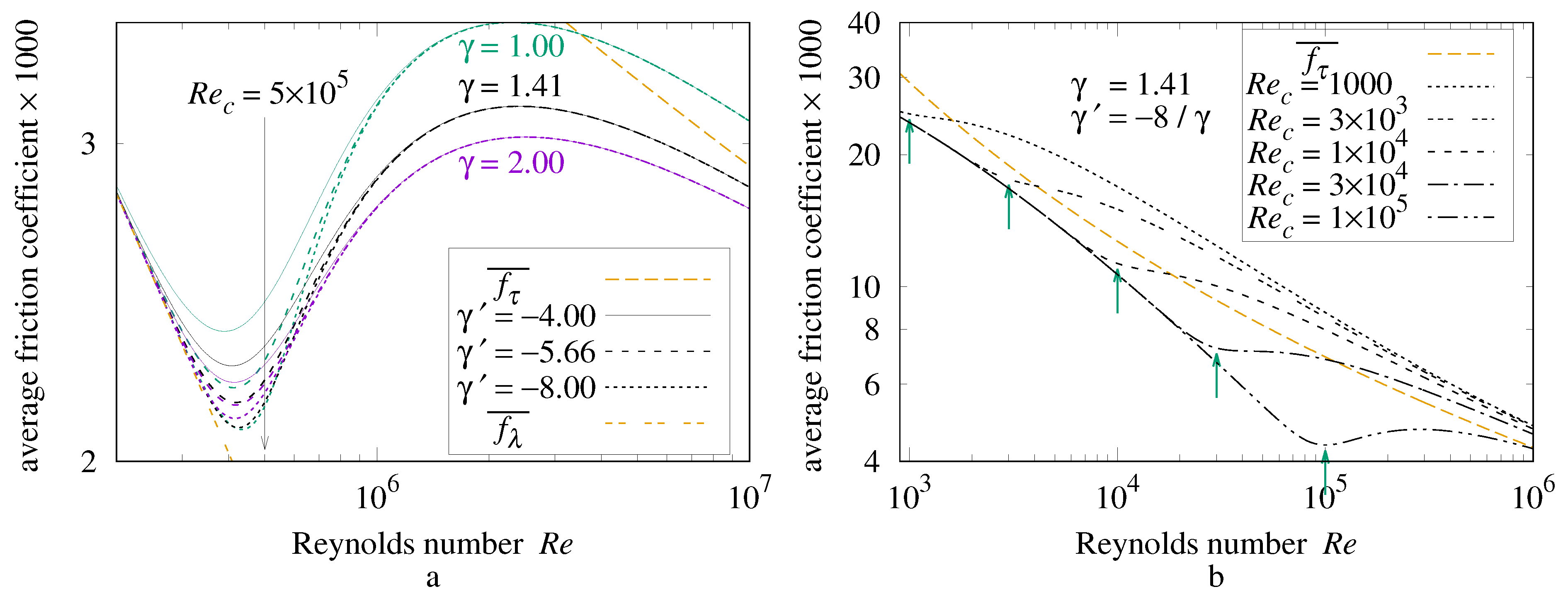
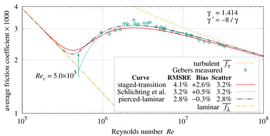
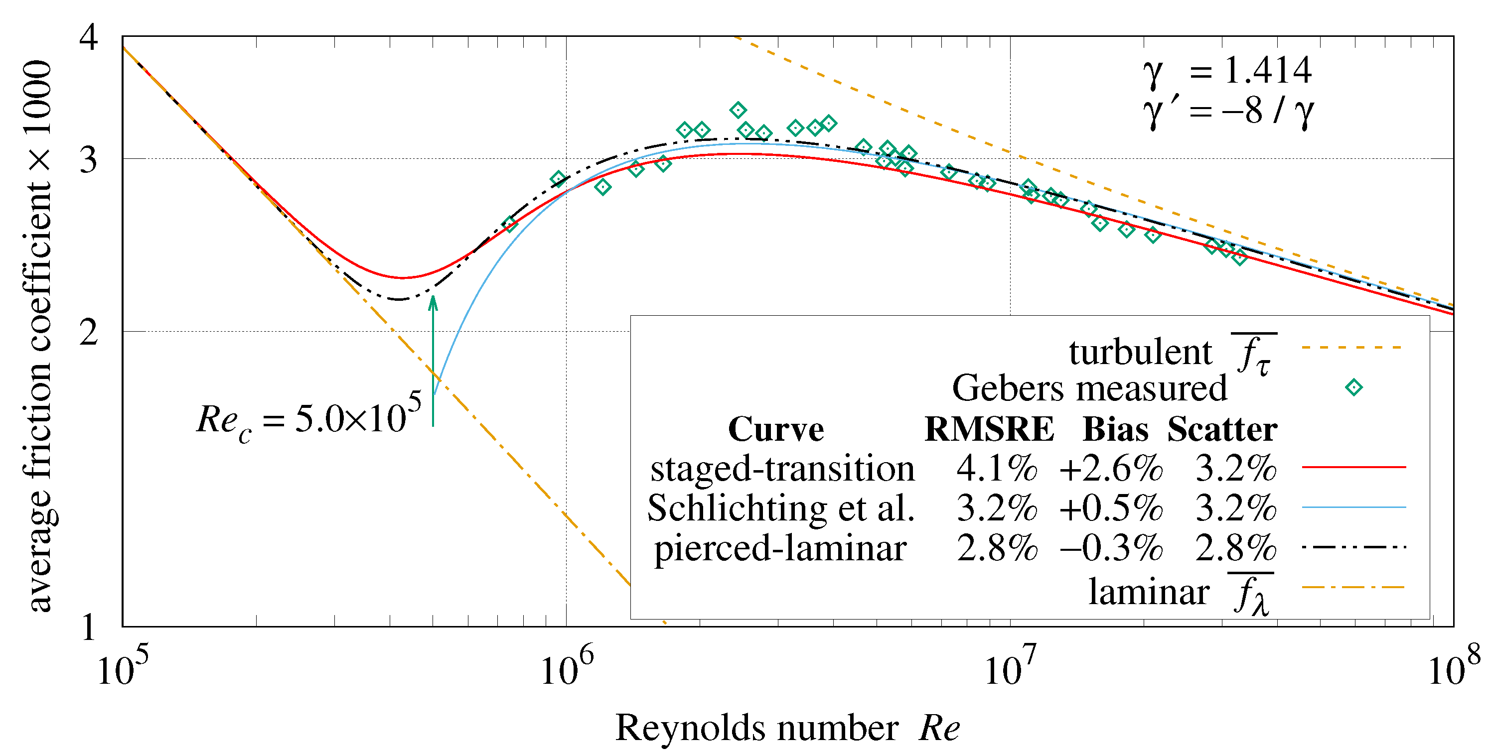
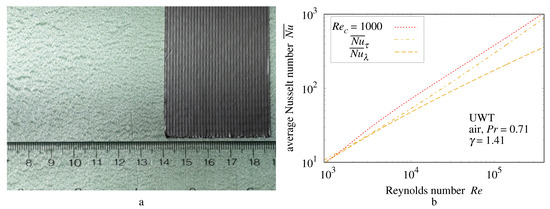
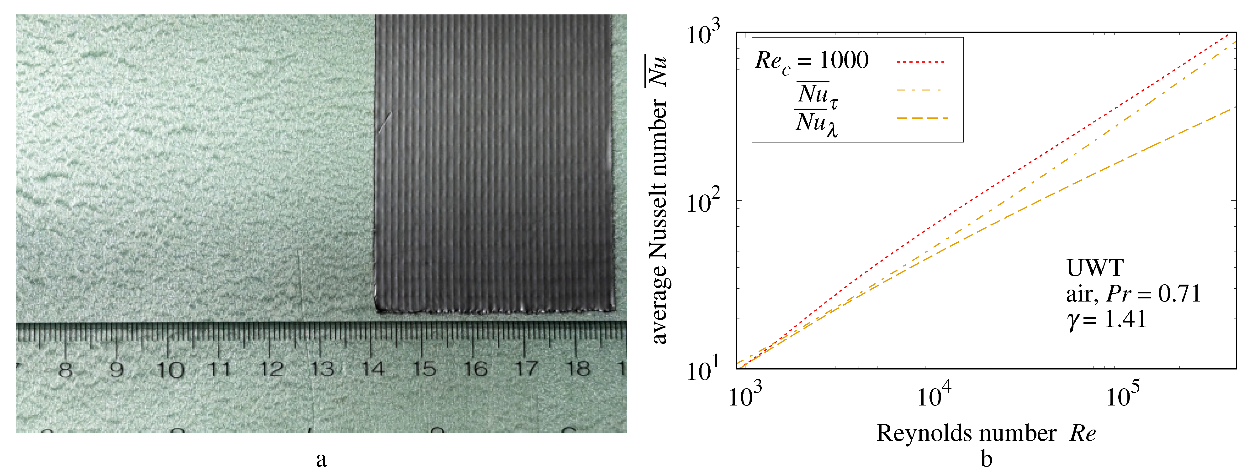
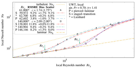
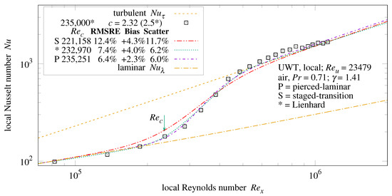
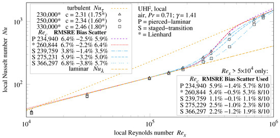
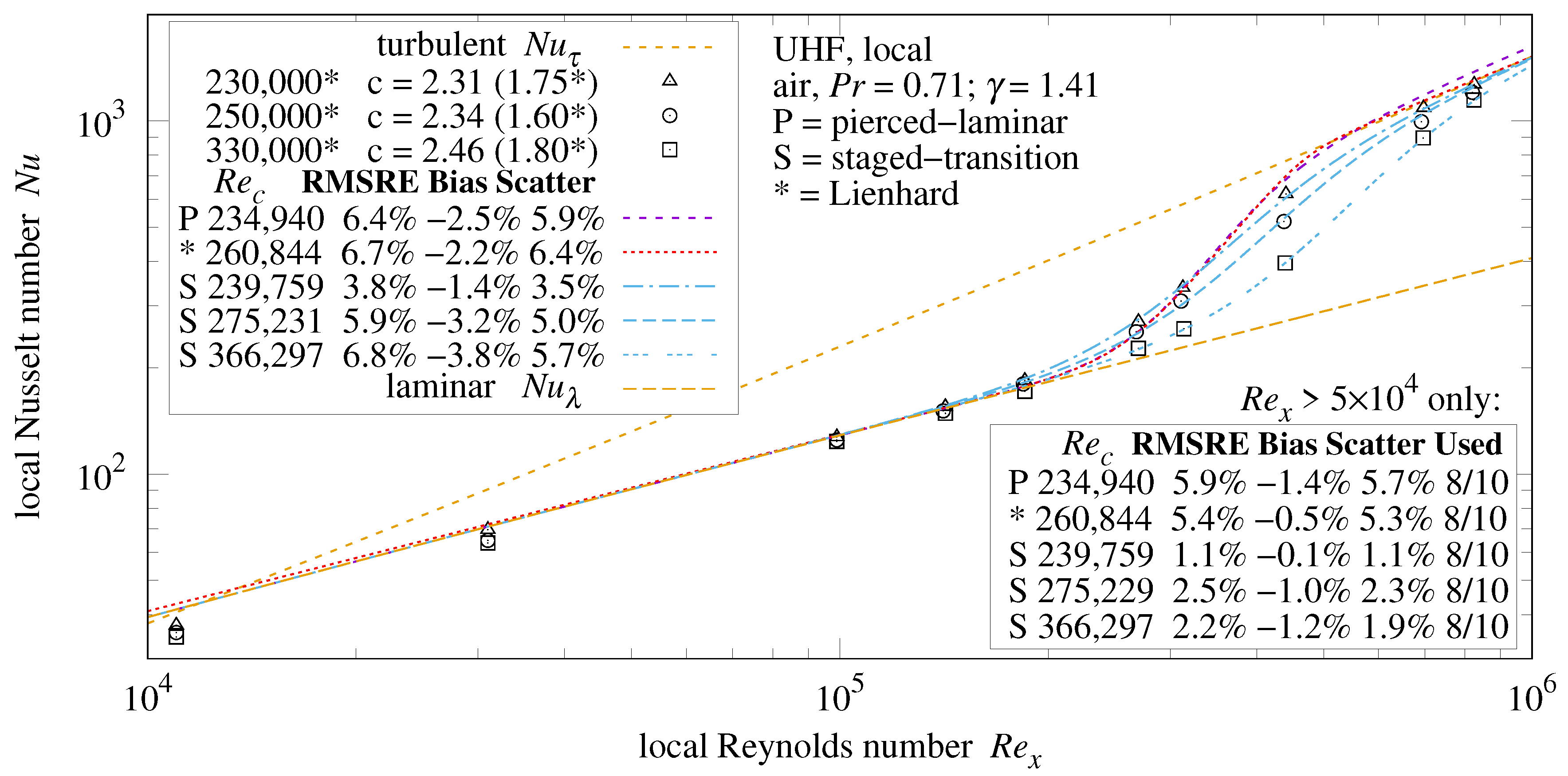
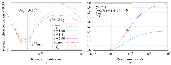
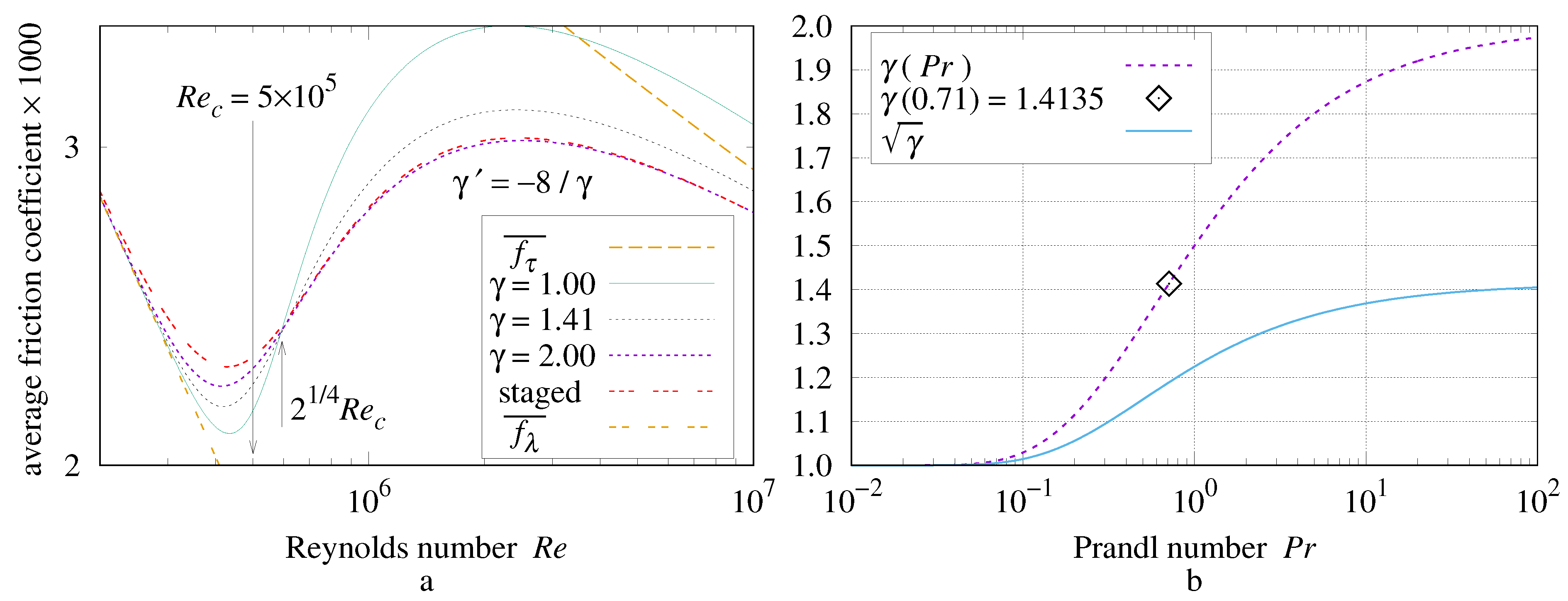
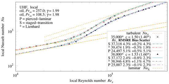
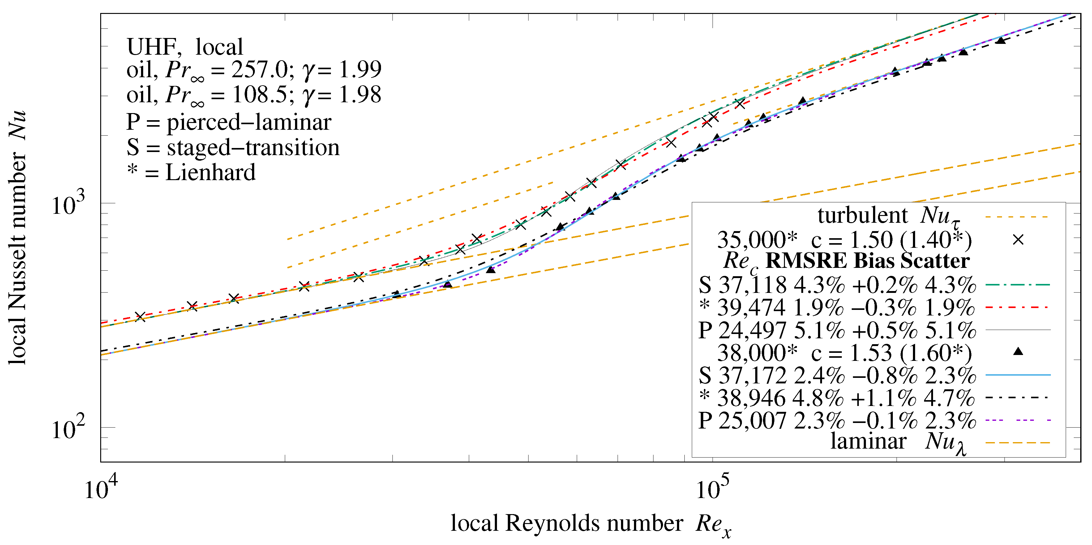
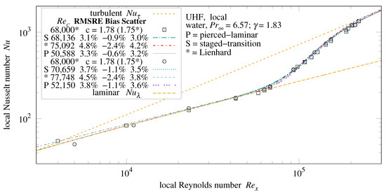
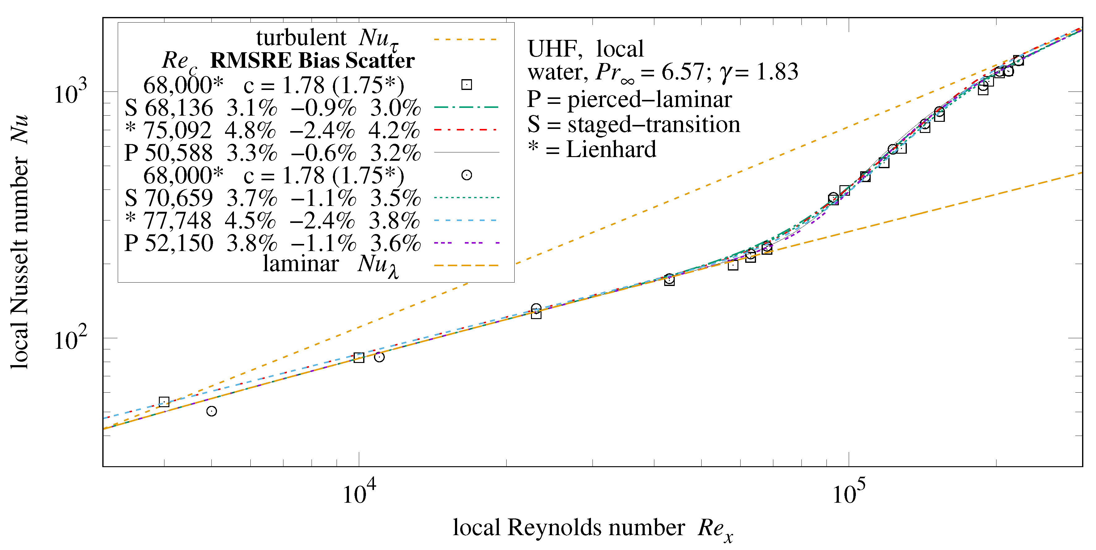
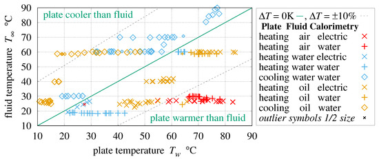
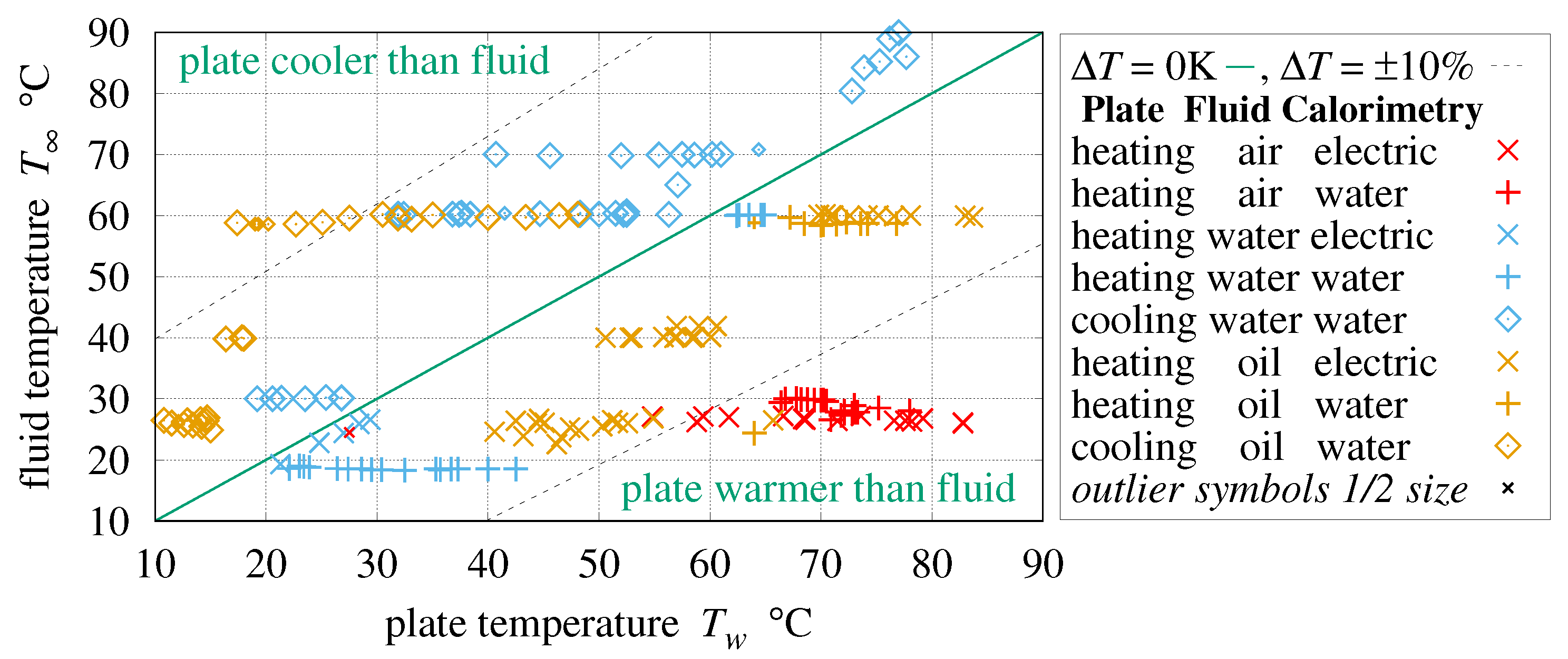
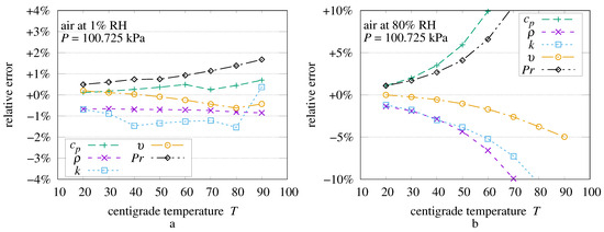
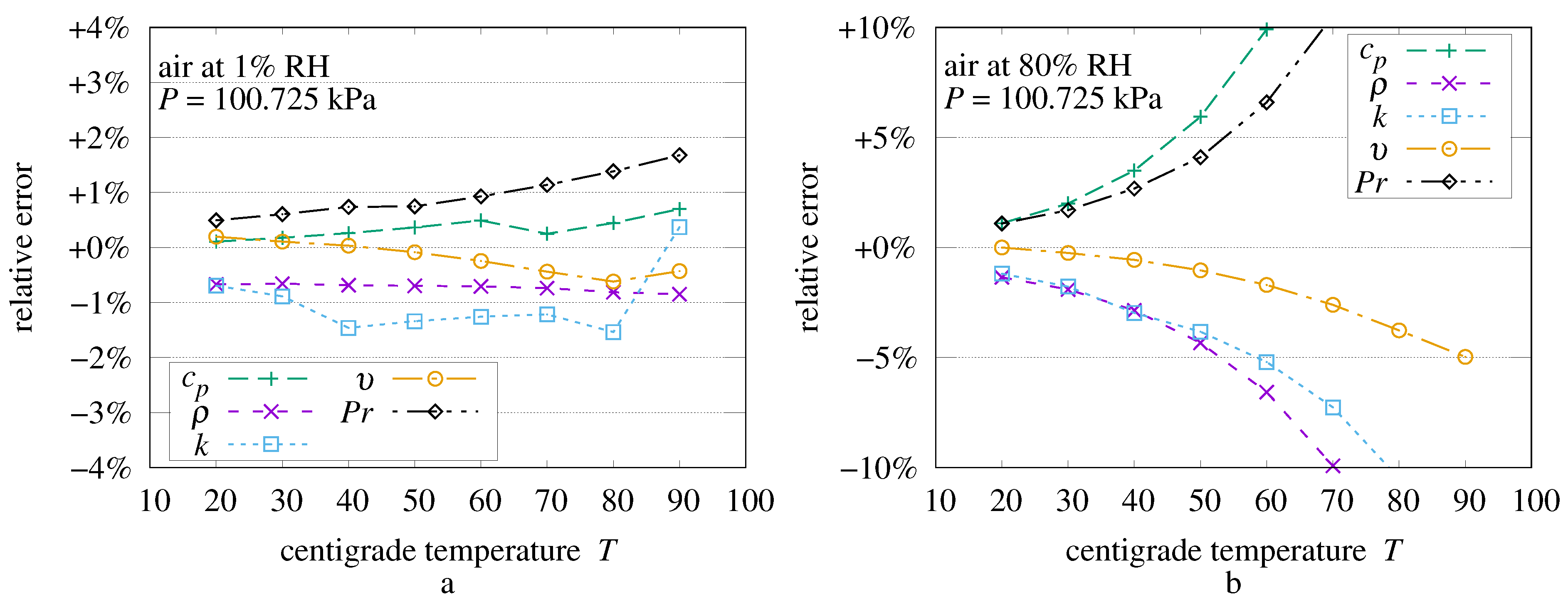
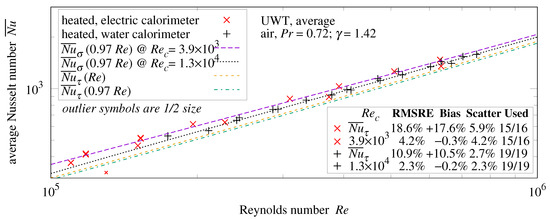
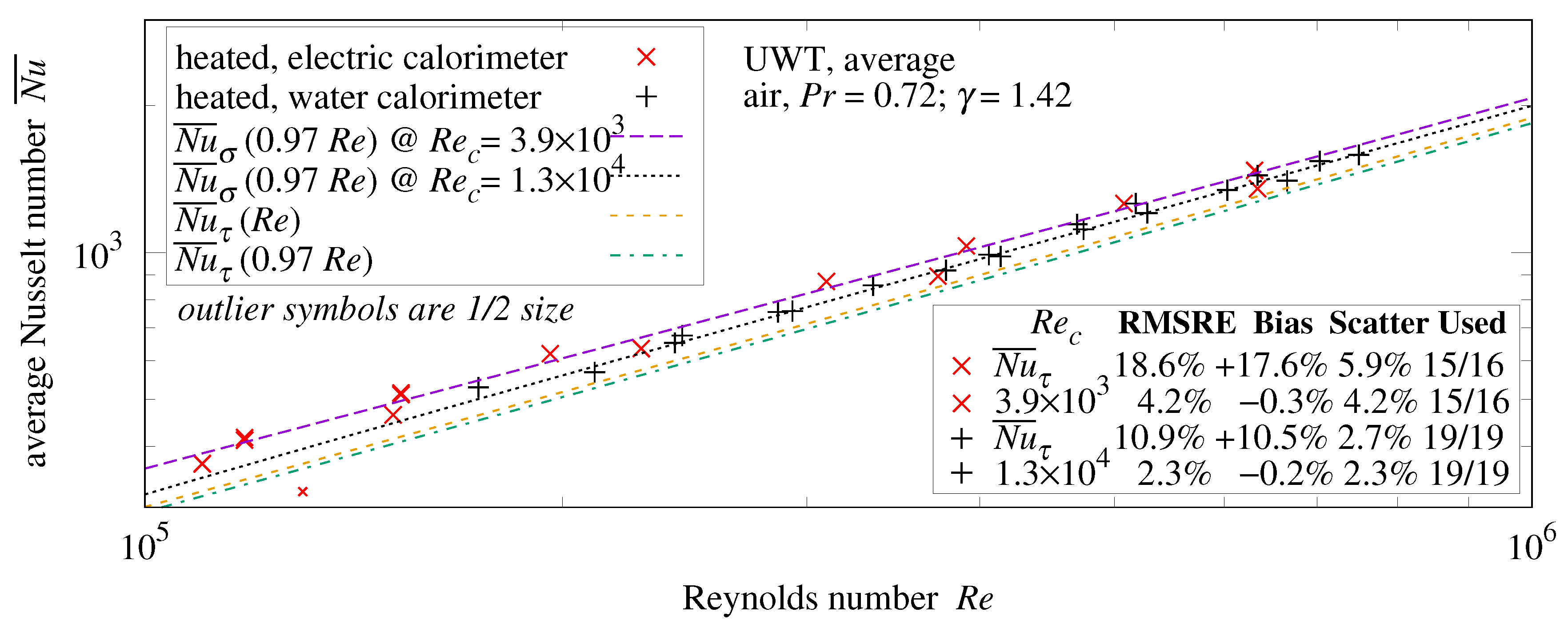
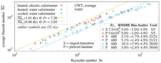
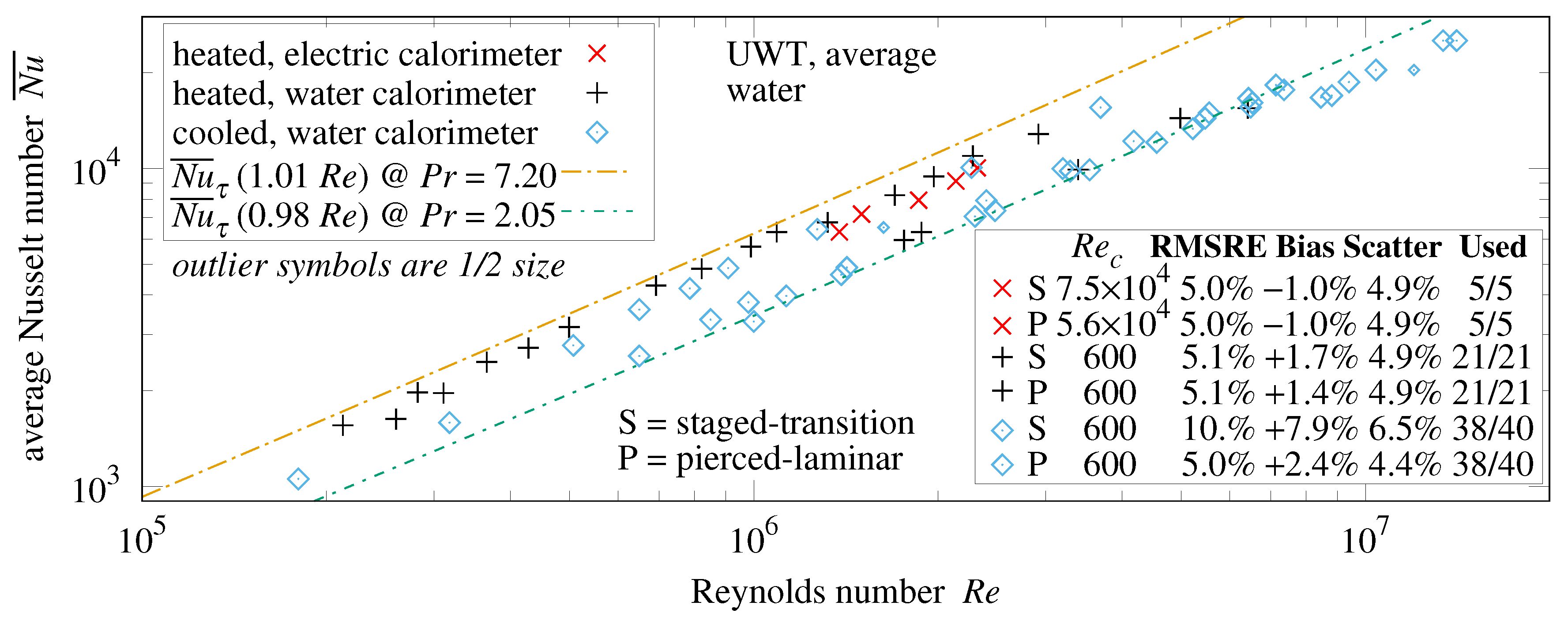
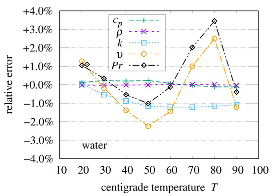
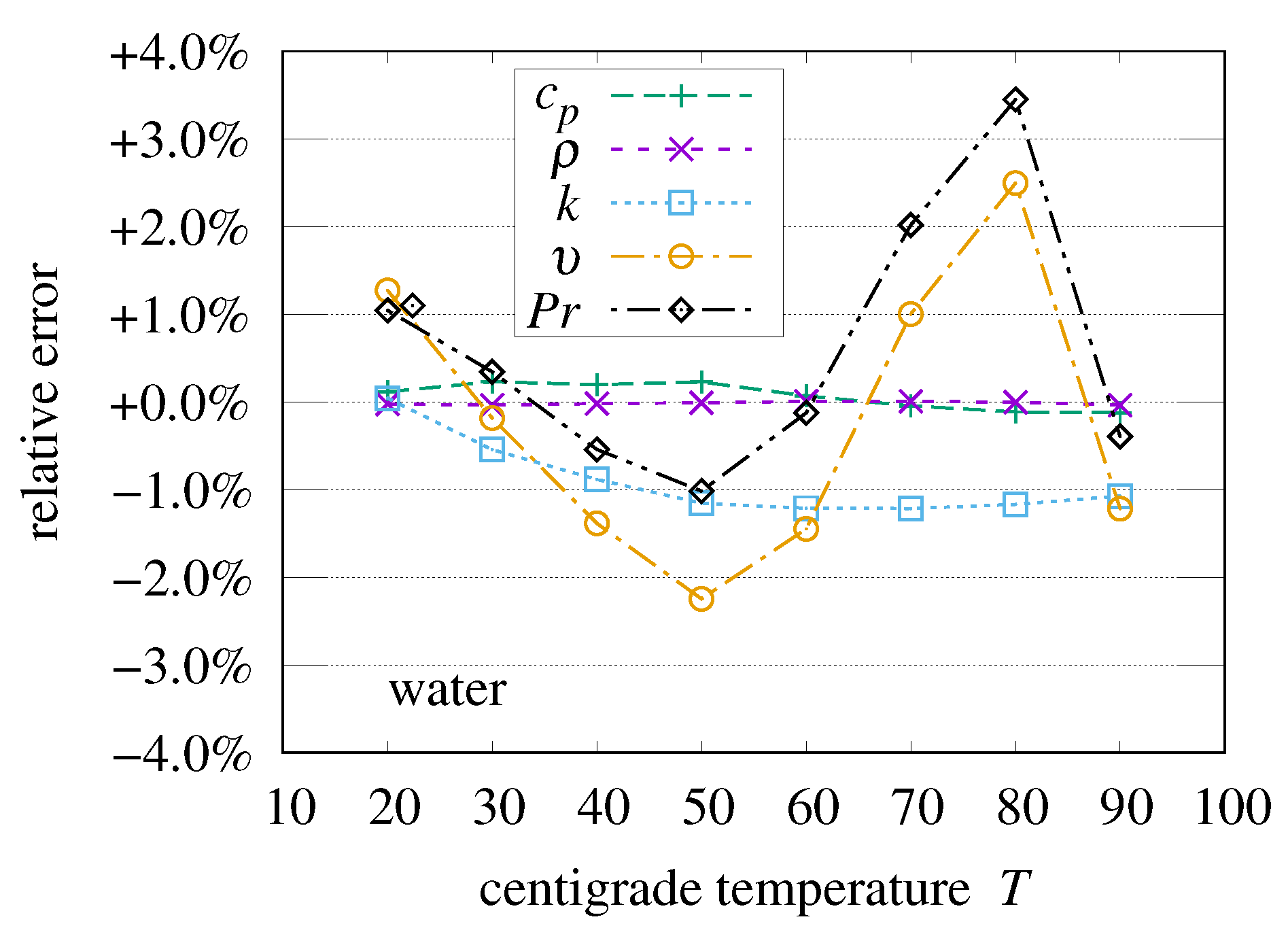
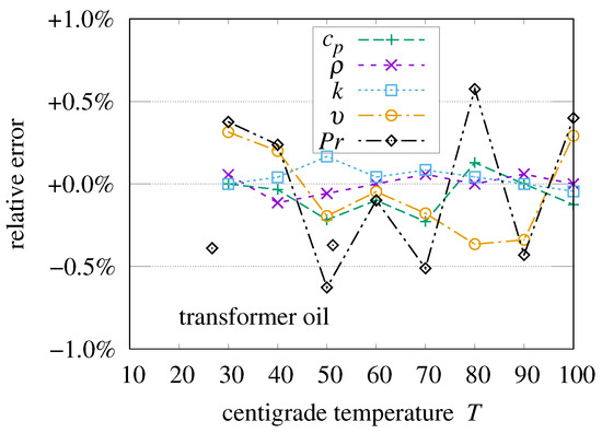
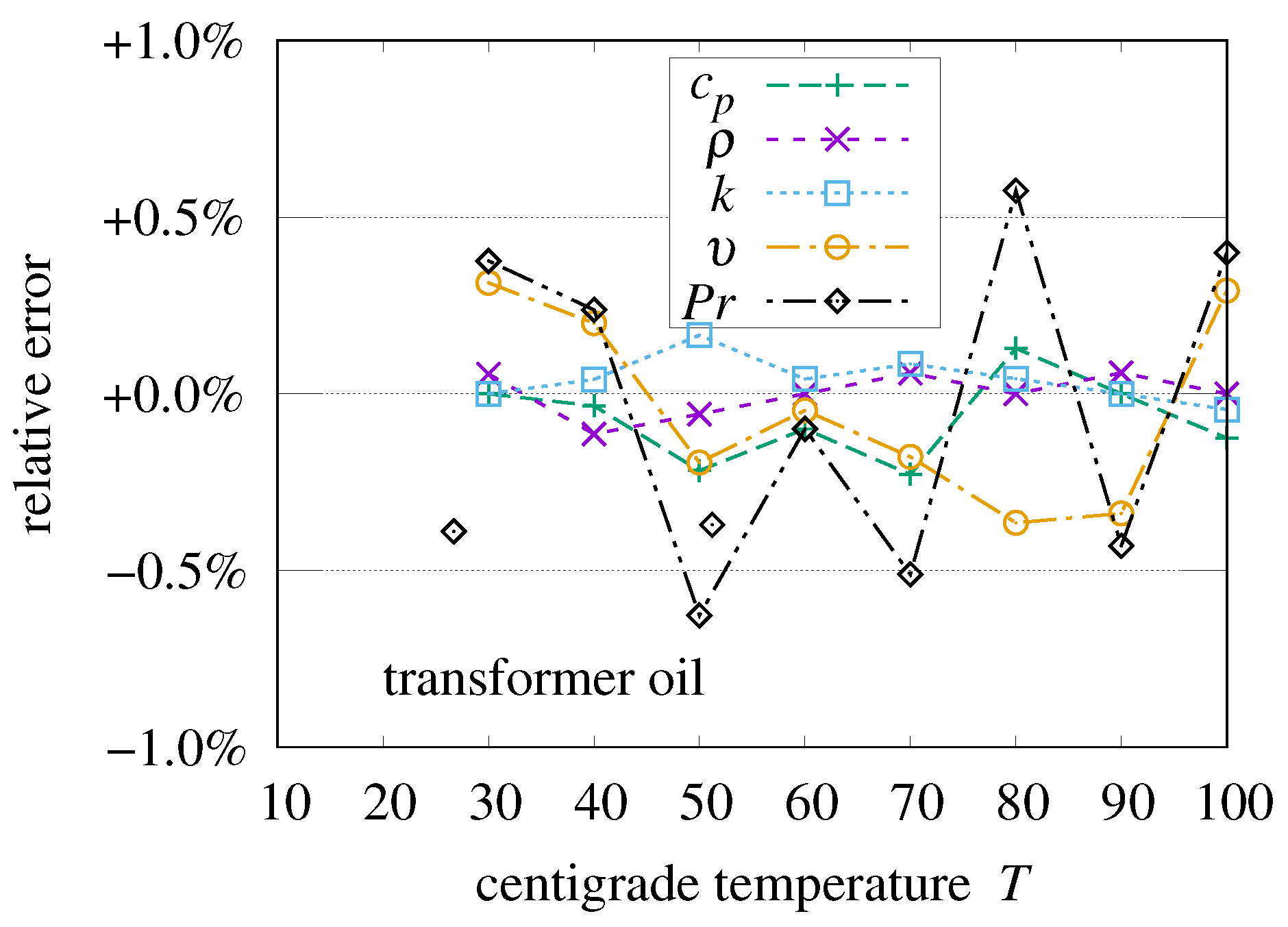
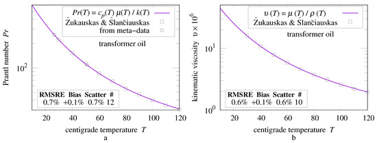
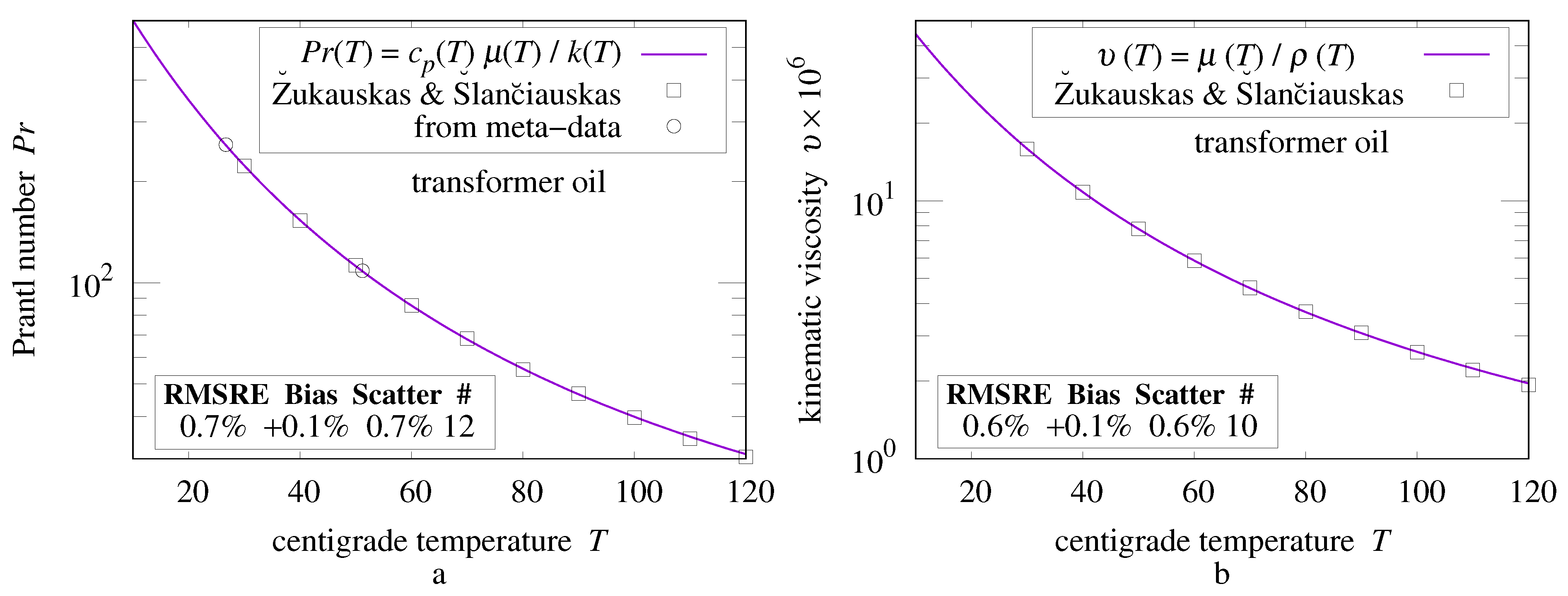
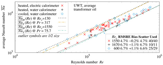
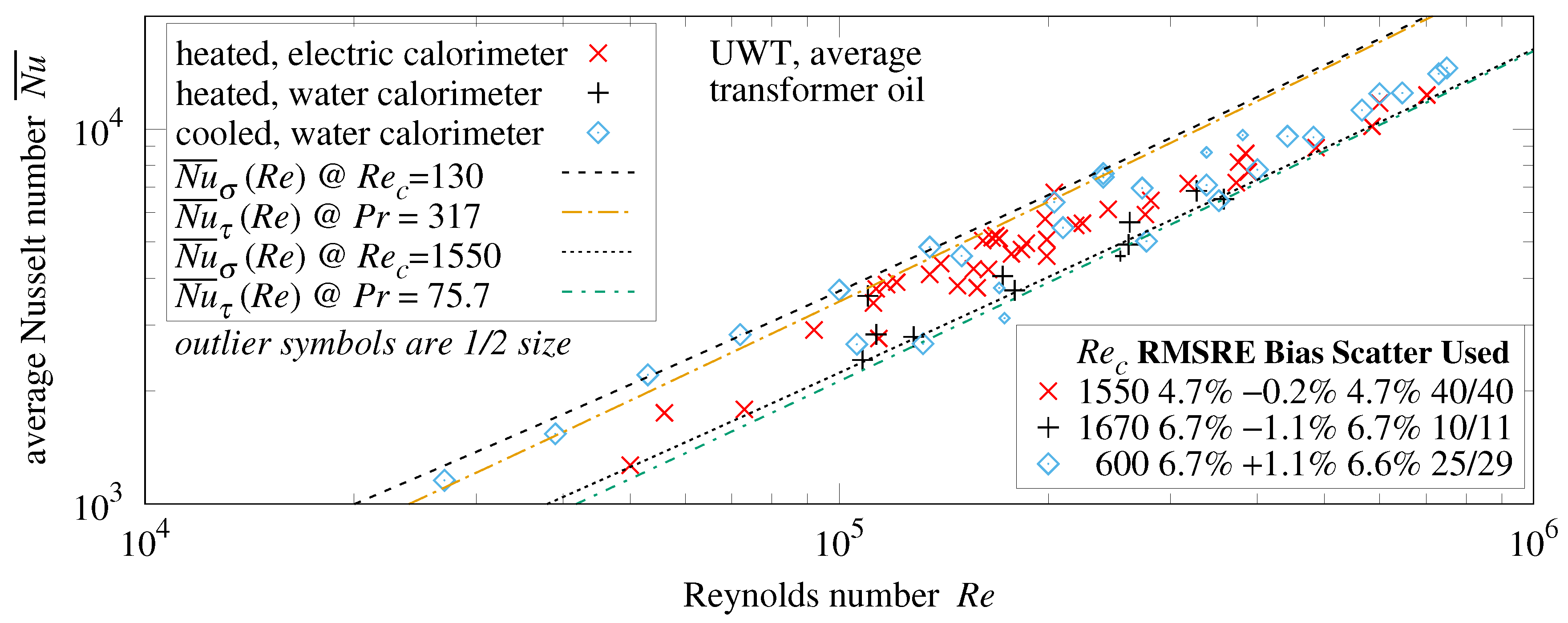

Disclaimer/Publisher’s Note: The statements, opinions and data contained in all publications are solely those of the individual author(s) and contributor(s) and not of MDPI and/or the editor(s). MDPI and/or the editor(s) disclaim responsibility for any injury to people or property resulting from any ideas, methods, instructions or products referred to in the content. |
© 2023 by the author. Licensee MDPI, Basel, Switzerland. This article is an open access article distributed under the terms and conditions of the Creative Commons Attribution (CC BY) license (https://creativecommons.org/licenses/by/4.0/).