Thermodynamic Modeling of the Uranium–Tellurium System: Estimation of the Uncertainties by a Bayesian Approach

Abstract

Under irradiation, the formation of fission products in the (U,Pu)O${}_2$ fuel with time has a substantial effect on its chemistry. In particular, migration of the most volatile fission products (Cs, Te, I, Mo) from the center to the periphery of the fuel pellet is induced by the large radial thermal gradient. To predict the thermodynamic properties of the irradiated fuel, thermodynamic modeling of the complex multi-component (Cs-I-Te-Mo)–(U-Pu)–O system is performed using the CALPHAD method. In this work, the thermodynamic assessment of the U–Te sub-system is performed. The literature review reveals a lack of experimental data as well as scattering and inconsistency of some of the data. In particular, no thermodynamic data exist on the liquid. From this review, input thermodynamic and phase diagram data are carefully selected. The Gibbs energy functions are then adjusted by fitting these data. An overall good agreement is obtained with all the selected data except for the enthalpy of formation for UTe which is underestimated by 13% by our model. This could be due to an inconsistency between the enthalpy of formation and vapor pressure data. In a second step, the uncertainties on the thermodynamic parameters and their propagation on the calculated thermodynamic and phase diagram data are estimated using a Bayesian approach. The analysis shows that there are too many parameters (22) for too few data points (120 points). The uncertainties are thus large on some of the calculated data. Moreover the inconsistency of some of the data and the lack of thermodynamic data for the liquid makes the model uncertain. New experimental data such as heat capacity, enthalpy of formation for the compounds, and chemical potentials or activities for the liquid phase would improve the reliability of our model. Measurements of phase diagram data in the U–UTe${}_2$ region are also required. However this work provides the first detailed uncertainty analysis of the U–Te CALPHAD model. Moreover our approach, contrary to other Bayesian methods, provides an analytical posterior probability distribution and analytical credible intervals for the calculated thermodynamic quantities. It also speeds up the simulation of the uncertainty estimations on the phase diagram.

1. Introduction

In sodium-cooled fast reactors (SFR), the fuel pins are made of uranium and plutonium dioxide (U,Pu)O${}_2$ pellets stacked in steel cladding. These fuel pellets undergo a large radial thermal gradient with a temperature of about 2200 K in the center and 850 K in the rim. Numerous fission products (FPs) are produced in the fuel through the fission nuclear reactions. Among these fission products, the most volatile ones such as iodine, cesium, tellurium, and molybdenum migrate from the center to the periphery of the fuel pellet and form a layer enriched in these fission products, the so-called “Joint-Oxyde-Gaine” or JOG [1,2]. With time, these fission products can attack the steel cladding to form the so-called “Reaction-Oxyde-Gaine” or ROG, which is a limiting factor for the cladding lifetime. To supply the models predicting the JOG and ROG layer thickness, the TAF-ID (Thermodynamics of Advanced Fuels–International Database [3]) thermodynamic database is being developed on the (U-Pu-O)–(I-Cs-Te-Mo)–(Fe-Cr-Ni) system using the CALPHAD method [2,3].

In the CALPHAD method [4], the Gibbs energies of all the phases (solids, liquid, gas) in the binary and ternary sub-systems are described as a function of temperature, composition, and pressure (only for the gas phase). By extrapolation from the sub-systems, the thermodynamic equilibrium in a multi-component system can then be calculated by minimizing the total Gibbs energy of the system. This powerful method has been extensively used since the ’80s to calculate phase equilibria and thermodynamic properties of multi–component systems. In these models, the thermodynamic parameters are assessed by fitting the available phase diagram and thermodynamic data. Nevertheless, the propagation of these fitting data uncertainties onto the thermodynamic parameters featured in the Gibbs energy functions in the CALPHAD models are rarely estimated. A few works have been published on this topic, see [5,6,7] for the most recent analyses. Moreover the propagation of these uncertainties on the calculated phase diagram and thermodynamic data are almost never determined. However it is crucial to estimate these uncertainties, in particular when these models are used in multi-physics codes like for instance the Fuel Performance Codes (ALCYONE and GERMINAL) which is used to simulate the thermo-mechanical behavior of a fuel pin [1,2]. The influence of these uncertainties on the physical properties and the behavior of the fuel (margin to the melting, thermal conductivity, …) has to be studied.

In the present work, the thermodynamic modeling of the U–Te binary sub-system is first performed using the PARROT module in the Thermo-Calc software [8]. In a second step, a Bayesian approach is applied to estimate the uncertainties on the thermodynamic parameters and their propagation on the calculated phase diagram and thermodynamic data.

The state of the art on the crystal structure data of the U${}_x$Te${}_y$ compounds, the phase diagram, and thermodynamic data is first presented in Section 2. The models to describe the Gibbs energy of the phases are described in Section 3. From these selected data and Gibbs energy models, a least-square method is applied to assess the Gibbs energy functions of the phases. In Section 4, the results of the fitting procedure are presented and the uncertainties on the assessed thermodynamic parameters are estimated using a Bayesian approach. Their propagation on the calculated thermodynamic and phase diagram data is then described. Finally, all the results are discussed.

2. State of the Art on the U–Te System and Selection of the Data for the Assessment

In this section, the crystal structure and thermodynamic data on the U${}_x$Te${}_y$ compounds and the phase diagram information are reviewed. From this critical review, the input data for the optimization procedure are selected.

2.1. Crystal Structure Data

Numerous compounds exist in the U–Te system: U${}_{10}$Te, UTe, U${}_3$Te${}_4$, U${}_2$Te${}_3$, U${}_3$Te${}_5$, U${}_7$Te${}_{12}$, $\beta$-UTe${}_2$, $\alpha$-UTe${}_2$, U${}_2$Te${}_5$, UTe${}_3$, U${}_2$Te${}_7$, UTe${}_5$. In 1993, Okamoto [9] reviewed the crystal structure data on the compounds. The data are reported in

Table 1. Crystal structure data on the phases of the U–Te system. The compounds in bold are considered in the present work. The compounds in italic gray${}^{\star }$ are not taken into account.

Compounds	Composition At. % Te	Space Group	Reference
$\gamma$-U	0	$\mathbf{Im}\overline{\mathbf{3}}\mathbf{m}$	Okamoto (1993) [9]
$\beta$-U	0	$\mathbf{P}{\mathbf{4}}_{\mathbf{2}}/\mathbf{mmm}$	Okamoto (1993) [9]
$\alpha$-U	0	Clcl	Okamoto (1993) [9]
U${}_{\mathit{10}}$Te${}^{\star }$	9	$Fm-3m$	Okamoto (1993) [9]
UTe	50	Fm-3m	Hermannsdörfer et al. (2006) [10]
U${}_{\mathbf{3}}$Te${}_{\mathbf{4}}$	57.1	I-43d	Solvyanskikh et al. (1977) [14]
U${}_{\mathbf{2}}$Te${}_{\mathbf{3}}$	60	Pnma	Tougait et al. (2001) [11]
U${}_{\mathbf{3}}$Te${}_{\mathbf{5}}$	62.5	Pnma	Tougait et al. (2001) [11]
U${}_{\mathit{7}}$Te${{}_{\mathit{12}}}^{\star }$	63.2	$P-6$	Tougait et al. (1998) [15]
$\beta$-UTe${}_{\mathbf{2}}$	66.7	Unknown	Okamoto (1993) [9]
$\alpha$-UTe${}_{\mathbf{2}}$	2	2	Stöwe (1996) [12]
U${}_{\mathbf{2}}$Te${}_{\mathbf{5}}$	71.4	C12m1	Tougait et al. (1997) [16]
UTe${}_{\mathbf{3}}$	75	$\mathbf{P}{\mathbf{12}}_{\mathbf{1}}/\mathbf{m}\mathbf{1}$	Stöwe (1996) [12]
U${}_2$Te${{}_7}^{\star }$	77.8	Unknown	Okamoto (1993) [9]
UTe${}_{\mathbf{5}}$	83.3	Pnma	Boehme et al. (1992) [17]
Te	100	$\mathbf{P}{\mathbf{3}}_{\mathbf{1}}\mathbf{21}$	Okamoto (1993) [9]

based on the most recent works of Hermannsdörfer et al. [10] for UTe, Tougait et al. [11] for U${}_2$Te${}_3$ and U${}_3$Te${}_5$ and Stöwe [12] for $\alpha$-UTe${}_2$ and UTe${}_3$.

In the review by Okamoto [9], U${}_7$Te${}_{12}$ is reported instead of U${}_3$Te${}_5$ in the phase diagram. The author argued that the structure of U${}_3$Te${}_5$ was not well defined. Later, Tougait et al. [11] investigated the crystal structure of both U${}_3$Te${}_5$ and U${}_2$Te${}_3$ by neutron diffraction. Thus based on these updated data, the compound U${}_3$Te${}_5$ is finally considered instead of U${}_7$Te${}_{12}$. Nevertheless, it is not clear whether this compound is stoichiometric or exhibits a small composition range. Due to the lack of reliable data, U${}_3$Te${}_5$ will be considered as a stoichiometric compound in the present work.

The high temperature $\beta$-UTe${}_2$ form was reported in the phase diagram of Slovyanskikh et al. [13] whose experimental work clearly showed an allotropic transition for this compound. However, the crystal structure of the $\beta$ form is not known.

The possible existence of U${}_2$Te${}_7$ was reported in the phase diagram of Okamoto [9]. However, due to the lack of data, it is not considered in the present work.

The compounds highlighted in bold in Table 1 are considered in our model. Due to the lack of reliable data on compounds composition range, only stoichiometric compounds are considered in the present work.

2.2. Phase Diagram Data

The phase diagram data coming from the literature are summarized in

Table 2. Phase diagram data on the U–Te system.

Composition Range At. % Te	Method	Reference	Comments
58–100	DTA, XRD	Slovyanskikh et al. (1968) [13]	Selected
0–65	DTA, XRD	Ellert et al. (1975) [18]	Selected
0–100	Review	Czechowitz (1985) [19]	Not selected
0–100	Review	Okamoto (1993) [9]	Not selected
100	Calphad model	Wolf (2017) [20]	Not selected

and reviewed in this section.

Slovyanskikh et al. [13] investigated the UTe–Te region using differential thermal analysis (DTA) and X-ray diffraction. From the DTA measurements, a eutectic reaction between UTe${}_5$ and Te and the peritectic decompositions of UTe${}_5$, UTe${}_3$, U${}_3$Te${}_7$, UTe${}_2$, and U${}_3$Te${}_5$ were highlighted. A polymorphic transition for UTe${}_2$ was also found to occur at 1125 °C. The compounds U${}_2$Te${}_3$, UTe${}_2$, U${}_3$Te${}_5$, U${}_3$Te${}_7$, UTe${}_3$, and UTe${}_5$ were identified using X-ray diffraction. A small region of homogeneity was assumed for UTe${}_2$ and U${}_3$Te${}_5$. Finally, liquidus temperatures were carefully measured from UTe${}_2$ to Te.

The U rich region from 0 to 65 at. % Te was later investigated using the same methods by Ellert et al. (1975) [18]. The melting point of uranium monotelluride was measured at 1730 °C. The authors reported that the temperature of the eutectic between U and UTe measured at 1180 °C was probably overestimated due to a partial dissolution of the crucible material. Liquidus temperatures were also determined. In the UTe–Te region, the authors mention that the results obtained in the range 50–57.2 at. % Te are uncertain. The U${}_3$Te${}_4$ compound was assumed to decompose by a peritectic reaction at 1540 °C. The range 57.2–60 at. % Te was found to be a single phase region (with Th${}_3$P${}_4$ crystal structure) with U${}_3$Te${}_4$ and U${}_2$Te${}_3$ as boundary compositions. A peritectic decomposition temperature of 1500 °C was assumed for U${}_2$Te${}_3$. The peritectic decomposition of U${}_3$Te${}_5$ was measured at 1300 °C instead of 1260 °C by Slovyanskikh et al. [13]. The authors in [13] suggest the existence of a small composition range for U${}_7$Te${}_{12}$ between 63.2–63.8 at. % Te given their results with X-ray diffraction.

In 1985, Czechowicz [19] proposed a phase diagram based on the data of Slovyanskikh et al. [13].

A phase diagram of the U–Te system was later proposed in the review by Okamoto in 1993 [9], mainly based on the experimental data of Ellert et al. (1975) [18]. Only the compounds U${}_7$Te${}_{12}$ and U${}_2$Te${}_5$ were considered instead of U${}_3$Te${}_5$ and U${}_3$Te${}_7$. A composition range was also represented for the UTe${}_2$ compound.

Recently, in 2017, Wolf [20] performed a thermodynamic assessment of the U–Te system using the Calphad method. The experimental data are not reported on the calculated phase diagram in [20]. However the calculated liquidus curve and the experimental data are not in good agreement.

In conclusion, the phase diagram is well established in the region from UTe${}_2$ to pure Te based on Slovyanskikh et al. [13]. However, the decomposition temperatures of the compounds and the liquidus data remain uncertain in the UTe–U${}_3$Te${}_5$ composition range. Moreover the liquidus in the U–UTe part is still not well known. For the optimization procedure, we selected only the experimental data measured by Slovyanskikh et al. [13] and Ellert et al. [18]. The compounds (in bold in Table 1) were selected and considered as stoichiometric in the present work.

2.3. Thermodynamic Data

All the data are reported in

Table 3. Thermodynamic data on the phases of the U–Te system. *: the condensed phases were not characterized. The reported phases by Czechowicz 1986 [22] were proposed on the basis of the phase diagram. The method DFT+U refers to the density functional theory + Hubbard model.

Thermodynamic Data	Phases	Method	Reference	Comments
$S_{298.15K}^0$	$\begin{array}{c}UTe,U_{3}T{e}_4,U_{2}T{e}_3\\ UT{e}_2,U_{2}T{e}_5,UT{e}_3\end{array}$	Estimation	Westrum 1962 [21]	Selected
$\Delta H_{f,298.15K}^0$	$UTe$, $U_{3}T{e}_4$	$\begin{array}{c}\mathrm{Direct}\mathrm{reaction}\\ \mathrm{calorimetry}\end{array}$	Baskin and Smith 1970 [23]	Selected
$\begin{array}{c}\Delta H_{f,298.15K}^0,S_{298.15K}^0\\ C_p\left(T\right),\Delta H_{fusion}\end{array}$	$\begin{array}{c}UTe,U_{3}T{e}_4,U_{2}T{e}_3,U_{3}T{e}_5\\ UT{e}_2,U_{2}T{e}_5,UT{e}_3,UT{e}_5\end{array}$	Estimation Solgasmix	Czechowicz 1985 [19]	$\begin{array}{c}\Delta H_{f,298.15K}^0\mathrm{selected}\\ \mathrm{except}UTe\mathrm{and}{U}_{3}T{e}_4\end{array}$
$p_{T{e}_2}$	*$UT{e}_3$/$U_{2}T{e}_5$	$\begin{array}{c}\mathrm{Quartz}\mathrm{membrane}\\ \mathrm{null}\mathrm{manometer}\\ \mathrm{Chemical}\mathrm{transport}\\ \mathrm{reaction}\end{array}$	Slovyanskikh et al., 1967 [27]	Selected
$p_{T{e}_2}$	*$UT{e}_2$/$U_{3}T{e}_5$	$\begin{array}{c}\mathrm{Bourdon}\mathrm{null}\\ \mathrm{manometer}\\ \mathrm{Chemical}\mathrm{transport}\\ \mathrm{reaction}\end{array}$	Sevast’yanov et al., 1971 [28]	Selected
$p_{Te}$, $p_{T{e}_2}$	$U_{3}T{e}_4$/$UTe$	KEMS	Czechowicz 1986 [22]	Selected
$\begin{array}{c}\Delta H_{f,298.15K}^0,S_{298.15K}^0\\ C_p\left(T\right)\end{array}$	$\begin{array}{c}UTe,U_{3}T{e}_4,U_{2}T{e}_3,U_{3}T{e}_5\\ UT{e}_2,U_{2}T{e}_5,UT{e}_3,UT{e}_5\end{array}$	Calphad model	Wolf 2017 [20]	Only $C_p\left(T\right)$ selected
$\Delta H_{f,0}^0$	$\begin{array}{c}UTe,U_{3}T{e}_4,U_{2}T{e}_3\\ U_{3}T{e}_5,U_{7}T{e}_{12},UT{e}_2\\ U_{2}T{e}_5,UT{e}_3,UT{e}_5\end{array}$	DFT+U	Qian et al., 2021 [25]	Not selected
$\Delta H_{f,0}^0$	$\begin{array}{c}UTe,U_{3}T{e}_4,U_{2}T{e}_3,U_{3}T{e}_5\\ UT{e}_2,U_{2}T{e}_5,UT{e}_3,UT{e}_5\end{array}$	DFT	OQMD [26]	Not selected

. No data exist on the liquid phase and very few measurements were performed on the solid compounds.

Westrum [21] estimated the standard entropies of UTe, U${}_3$Te${}_4$, U${}_2$Te${}_3$, UTe${}_2$, U${}_2$Te${}_5$, and UTe${}_3$ compounds.

There are not any heat capacity measurements. Only estimations are provided by Czechowicz [19] and Wolf [20]. The estimation values from Czechowicz [19] are significantly higher than those from Wolf [20] at high temperatures. Due to the lack of experimental data, the $C_p\left(T\right)$ data of Wolf [20] based on the Kopp–Neumann rule are considered in the present work for all compounds.

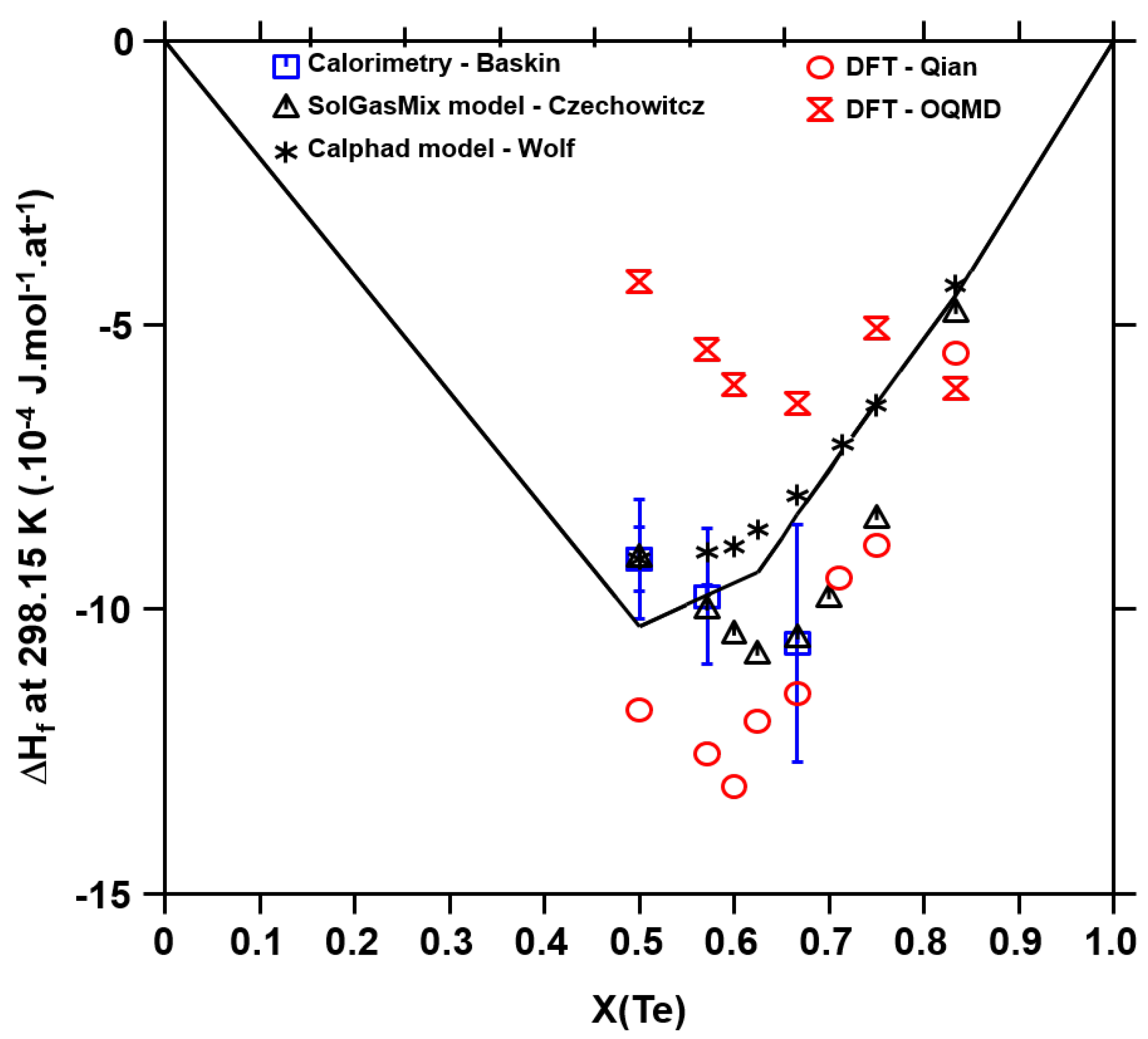
All the enthalpy of formation data are reported in Figure 1. The enthalpy of formation for UTe and U${}_3$Te${}_4$ was measured by direct-reaction calorimetry using a Calvet-type high-temperature liquid metal (tin) solution calorimeter. The values are equal to: −182.4 ± 11.3 kJ/mol for UTe and −228.0 ± 1.3 kJ/mol for UTe${}_{1.33}$. The enthalpy of formation for UTe${}_2$ was also estimated to be −318 kJ/mol by the authors assuming a linear relation to the Te/U ratio.

Czechowicz [22] reported uncertainties in the work of Baskin et al. [23] due to the uncertain percentage of each phase in the samples for calorimetric measurements. Later Mills [24] reviewed the data and assigned them larger uncertainties: −182.4 ± 20.9 kJ/mol for UTe and −684.1 ± 83.7 kJ/mol for U${}_3$Te${}_4$. These solely experimental data of Baskin et al. [23] for UTe, U${}_3$Te${}_4$ are selected in this work.

There are no other enthalpy of formation measurements. However in 1985, Czechowicz [19] published estimated thermodynamic data ($\Delta H_{f,298.15K}^0$, $S_{298.15K}^0$, $C_p\left(T\right)$, $\Delta H_{fusion}$) on UTe, U${}_3$Te${}_4$, U${}_2$Te${}_3$, U${}_3$Te${}_5$, UTe${}_2$, U${}_3$Te${}_7$, UTe${}_3$, and UTe${}_5$. The authors only mentioned that the thermodynamic data were obtained from the literature or estimated without any further explanation. Recently Wolf [20] derived a Calphad model on U–Te. The authors also reported thermodynamic data ($\Delta H_{f,298.15K}^0$, $S_{298.15K}^0$, $C_p\left(T\right)$) for the compounds. For all the compounds except UTe and U${}_3$Te${}_4$, the data of Czechowicz [19] were selected. The data of Wolf [20] were discarded due to the disagreement with the data of Baskin et al. [23] for U${}_3$Te${}_4$.

More recently, density functional theory (DFT) calculations were performed on U–Te compounds by Qian et al. [25]. Additionally, other DFT data are available in the OQMD database [26]. Very large discrepancies are found between both DFT studies. Moreover none of these studies are in agreement with the experimental data of Baskin et al. [23] for UTe, U${}_3$Te${}_4$, and UTe${}_2$. Therefore the DFT data were not used.

Measurements of Te${}_2$ equilibrium vapor pressure were performed in two phase regions: UTe${}_3$-U${}_2$Te${}_5$ by Slovyanskikh et al. [27] using a manometer, UTe${}_2$/U${}_3$Te${}_5$ by Sevast’yanov et al. [28] and in U${}_3$Te${}_4$/UTe by Czechowicz [22] by high temperature mass spectrometry. Czechowicz [22] provided a detailed description of their experimental conditions and results analysis. The authors reported the inconsistency of their results with the enthalpy of formation data of Baskin et al. [23]. However the large uncertainties in the experimental work of Baskin et al. [23] due to the unknown percentage of the phases in the calorimetric products was mentioned. All the vapor pressure data were used in the present work.

In conclusion, for the optimization procedure, we selected the heat capacity functions derived by Wolf [20], the experimental data of Baskin et al. [23] for the enthalpy of formation of UTe and U${}_3$Te${}_4$ and the estimated data of Czechowicz [19] for the other compounds. The only existing standard entropies estimated by Westrum [21] were also considered. Finally all the Te${}_2$ partial pressure data measurements by Slovyanskikh et al. [27], Sevast’yanov et al. [28], and Czechowicz [22] were used.

3. Thermodynamic Modeling with the CALPHAD Method

The Gibbs energy functions for all the phases of the uranium–tellurium system are described. Then the strategy for the optimization procedure with PARROT is explained.

3.1. Gibbs Energy Models

All the Gibbs energy functions are referred to the enthalpy of the pure elements in their stable state at 298.15 K and 1 atm (designated as $H_i^{SER}$). For the pure elements U and Te in their different states, the Gibbs energy functions are taken from the SGTE pure database [29].

For all the stoichiometric compounds, the Gibbs energy function is expressed as follows

$$G_m^{\varphi }-\sum _i{b}_i^{\varphi }{H}_i^{SER}=a_0+a_{1}T+a_{2}T\ln \left(T\right)+a_3{T}^2+a_4{T}^{-1}$$

(1)

where $b_i^{\varphi }$ is the stoichiometric factor of element i in the compound $\varphi$ and $a_n$ are unknown parameters to be estimated. For the U${}_x$Te${}_y$ compounds, the $a_n$ coefficients (with $n=2,3,4$) are fixed using the $C_p\left(T\right)$ functions provided by Wolf [20] assuming a Kopp–Neumann law.

For the liquid phase, the ionic two-sublattice model [30] is chosen to keep the consistency with the model for this phase in the TAF-ID database [3]. The sublattice model is the following one

$${\left(U^{+4}\right)}_P{(V{a}^{-Q},Te,UTe)}_Q.$$

In this model, uranium cation U${}^{+4}$ is in the first sublattice and charged vacancies (Va${}^{-Q}$), neutral Te and UTe species are introduced in the second sublattice. The site numbers P and Q are defined as the average charges of the second and first sublattices, respectively

$$\begin{array}{cc}\hfill & P=Q{y}_{V{a}^{-Q}}\hfill \\ \hfill & Q=4.\hfill \end{array}$$

(2)

The charge electroneutrality of the liquid phase is maintained by varying the charge –Q of the vacancies which varies with the composition in Te (or U). The Gibbs energy of the liquid phase is then expressed by

$$\begin{array}{cc}\hfill G_m^{liq}=& y_{Va}{G}_{\left(U^{+4}\right)\left(Va\right)}^{liq}+y_{Te}{G}_{Te}^{liq}+y_{UTe}{G}_{UTe}^{liq}+QRT\left(y_{Va}\ln y_{Va}+y_{Te}\ln y_{Te}+y_{UTe}\ln y_{UTe}\right)\hfill \\ \hfill & +y_{Va}{y}_{UTe}\left(L_{\left(U^{+4}\right)(Va,UTe)}^0+(y_{Va}-y_{UTe})L_{\left(U^{+4}\right)(Va,UTe)}^1+{(y_{Va}-y_{UTe})}^2{L}_{\left(U^{+4}\right)(Va,UTe)}^2\right)\hfill \\ \hfill & +y_{UTe}{y}_{Te}\left(L_{(UTe,Te)}^0+(y_{UTe}-y_{Te})L_{(UTe,Te)}^1+{(y_{UTe}-y_{Te})}^2{L}_{(UTe,Te)}^2\right).\hfill \end{array}$$

(3)

The interaction terms have a linear dependence in temperature defined by

$$L_{(UTe,Te)}^i=b^i+c^{i}T.$$

(4)

There are three end-members in the model: (U${}^{+4}$)${}_1$ (Va${}^{-1}$)${}_4$ corresponding to pure uranium liquid, pure tellurium liquid, and UTe liquid. The introduction of the UTe species is necessary to reproduce the shape of the phase diagram with a high melting point for UTe and a complex liquidus curve in the UTe–Te part. Moreover, a short-range ordering in the liquid is often observed in the Te-based systems which also justifies the introduction of UTe species even if there are no experimental evidence of its existence.

The interaction terms $L_{\left(U^{+4}\right)(Va,UTe)}^i$ and $L_{(UTe,Te)}^i$ allow the description of U–UTe and UTe–Te parts of the phase diagram, respectively.

Finally, the gas phase is described by an ideal mixing of gaseous species (Te, Te${}_2$, Te${}_3$, Te${}_4$, Te${}_5$, Te${}_6$, Te${}_7$, UTe, U) whose Gibbs energy functions ${}^o{G}_i^{gas}$ come from [31] for all species except for UTe [32]. The Gibbs energy is expressed as

$$G^{gas}=\sum _i{y}_i\left[{}^o{G}_i^{gas}-\sum _j{b}_{ij}{H}_j^{SER}+RT\ln y_i\right]+RT\ln \left(\frac{p}{p_0}\right)$$

(5)

where $y_i$ are the constituent fractions. Their sum is thus unity. $b_{ij}$ is the number of atoms j in the species i. The standard pressure $p_0$ is set to ${10}^5$ Pa. The partial pressure of species i $p_i$ is related to the constituent fraction by

$$p_i=y_{i}p$$

(6)

where p is the total pressure.

3.2. Optimization Procedure

As previously mentioned, the $C_p\left(T\right)$ functions provided by Wolf [20] were selected which allowed the $a_2$, $a_3$, and $a_4$ coefficients to be fixed for all the compounds. As there are no experimental data on the melting enthalpy of UTe, the value from the Solgasmix database published by Czechowicz (1985) [19] was taken.

A first set of parameters $(a_0,a_1)$ for UTe was assessed as well as the entropy of melting of the compound using the following data: $\Delta H_{f,298.15K}^0$, $S_{298.15K}^0$, $\Delta H_{fusion}$, and $T_{melting}$. The other compounds were progressively introduced and interaction parameters in the liquid were assessed to have a starting set of variables. All the compounds were forced to be stable at 298.15 K by setting their driving forces to be equal to 0. The optimization was then performed with PARROT to reproduce both the thermodynamic and phase diagram data. The weights on the different experimental data had to be adjusted to get a final good agreement with all the data within the error bars provided by the authors.

4. Use of Conjugate Prior Distribution for CALPHAD Modeling

In this section, the uncertainty quantification on the parameters is studied through a Bayesian approach for the CALPHAD modeling quantities. In the context of the CALPHAD modeling, the integration of the uncertainty study is still at its early stage. However we can quote the works of [5,6,7,33,34] in which the authors propose different methods to deal with uncertainty management using the Bayesian approach. A wider list of references can be found in ([35] Section III.3.3) as well as a more global description of the methods used in these works.

In the following, we will consider the unknown parameters to be real random quantities and we will denote them with capital letters, that is $A_0$ and $A_1$ for the random unknown quantities in the Gibbs energy model (1) and $B^i$ and $C^i$ for the parameters in the interaction term $L^i$. In the following, $\mathbb{E}\left[X\right]$ denotes the expectation (or mean value) of a real random variable X and $\mathrm{Var}\left(X\right)$ its variance, that is respectively the average value of X and the average of the squared distance ${(X-\mathbb{E}\left[X\right])}^2$. We also recall that the covariance between two real random variables X and Y is defined by

$$\mathrm{Cov}(X,Y)=\mathbb{E}\left[(X-\mathbb{E}[X\left]\right)(Y-\mathbb{E}[Y\left]\right)\right].$$

(7)

When considering a set of several random variables, one can extend the definitions of variance and covariance for this group of variables. This defines the covariance matrix, which is the matrix that features the variance of each random and the pair-wise covariances.

4.1. Bayesian Inference

Before getting to the details of the method used in this work, some general description of the Bayesian framework is presented in this section. Notice that we do not provide a comprehensive description here. The interested reader is referred to Robert’s book [36] for a more complete description of the Bayesian framework.

Parametric models such as Gibbs energy models (1) are fitted with a sample of data. One can measure the goodness-of-fit with respect to such data via the so-called likelihood function. As we consider a parametric model, the goodness-of-fit value is calculated for given values of the unknown parameters $A_n$ and given the fitting data values.

In the Bayesian approach of such parametric models, we consider that there exists a prior knowledge on the parameters of interest $A_n$, that is to say that there exists an expert advice about the values that $A_n$ can take. The Bayesian inference allows the integration of such anterior knowledge on $A_n$. Such knowledge is called the prior probability distribution of the random variables $A_n$.

Thanks to Bayes’ theorem, these two quantities—the prior probability distribution and the likelihood function—enable to determine the posterior probability distribution. This posterior probability distribution gives the distribution of the parameters values, provided that the experiments results are known. Put in another way, this posterior probability distribution determines what values of the parameters have the most likely outcome when knowing the values of the experiments and their experimental uncertainty.

4.2. Conjugate Prior Probability Distribution

The specificity of the approach used here is the use of the so-called conjugate prior probability distribution. Usually, the determination of the posterior probability distribution can be difficult and or numerically expensive. However, there exists some prior probability distribution that works well with some models. It is the case when considering a Gaussian prior probability distribution with a linear model: the Gaussian distribution remains Gaussian when a linear transformation is applied, see for example [37] for more details. This famous result from statistics is well adapted to the case of the CALPHAD modeling as the Gibbs energy model (1) is linear with respect to the parameters $A_n$. In this specific case, we can get a Gaussian posterior probability distribution. Notice that, apart from some cases, there is no guarantee to obtain an analytical posterior probability distribution. In [35] the author studies the specific use of conjugate prior for the CALPHAD models.

Another interesting result is that a Gaussian distribution is entirely defined by its mean value and its variance. In the case of conjugate prior probability distribution, a closed form expression is known for the posterior mean $\mathit{\nu }$ and the posterior covariance matrix $\mathbf{S}$. They are given by the following matrix expressions

$$\mathbf{S}={\left({\mathbf{D}}^t{\mathbf{s}}_{\mathbf{Z}}^{-1}\mathbf{D}+{\mathbf{s}}_{\mathbf{0}}^{-1}\right)}^{-1}$$

(8)

and

$$\mathit{\nu }=\mathbf{S}\left({\mathbf{D}}^t{\mathbf{s}}_{\mathbf{Z}}^{-1}\mathbf{Z}+{\mathbf{s}}_{\mathbf{0}}^{-1}{\mathit{m}}_{\mathbf{0}}\right)$$

(9)

where ${}^t$ denotes the matrix transposition operator and where ${\mathbf{s}}_{\mathbf{Z}}^{-1}$ represents the inverse of the matrix ${\mathbf{s}}_{\mathbf{Z}}$. In the above expressions, the prior mean and the prior covariance matrix are denoted by ${\mathit{m}}_{\mathbf{0}}$ and ${\mathbf{s}}_{\mathbf{0}}$ respectively, the fitting data are denoted by $\mathbf{Z}$ and the experimental uncertainties are denoted by ${\mathbf{s}}_{\mathbf{Z}}$. Finally, $\mathbf{D}$ is the design matrix, that is the evaluated functions that multiply each parameter. See [35] for more details about the conjugate prior probability distribution approach for the CALPHAD models.

Finally, the adequacy between the number of model parameters and the degree of freedom of the fitting data has been tackled in this work. This study relies on well-known results from linear algebra and is beyond the scope of this paper. However, some details can be found in the Appendix A.

4.3. Uncertainty on the Calculated Thermodynamic Quantities

In this section, we explain how to get the posterior probability distribution on calculated thermodynamic data once we obtain the posterior probability distribution of the unknown parameters. We specify how the posterior probability distribution is determined for some specific quantities. Such quantities are the enthalpies of formation for the compounds UTe, U${}_3$Te${}_4$, U${}_2$Te${}_3$, U${}_3$Te${}_5$, UTe${}_2$, U${}_2$Te${}_5$, UTe${}_3$ and UTe${}_5$; the entropies for UTe, U${}_3$Te${}_4$, U${}_2$Te${}_3$, UTe${}_2$, U${}_2$Te${}_5$ and UTe${}_3$ compounds and the partial pressures for the two-phases regions (UTe + U${}_3$Te${}_4$), (U${}_3$Te${}_5$ + UTe${}_2$) and (U${}_2$Te${}_5$ + UTe${}_3$). The results given in the following subsections will be used in Section 5 for the comparisons of the posterior prediction and the posterior prediction error with the experiments.

4.3.1. Enthalpy of Formation

Recall the chosen model (1) for the Gibbs energy functions of each compound, it is well known that the enthalpy of formation at temperature $T_0$ = 298.15 K of such compound is given by

$$\Delta H_{f,T_0}^0=A_0-a_2{T}_0-a_3{T}_0^2+2a_4{T}_0^{-1}.$$

(10)

Recall that the parameters $a_2$, $a_3$, and $a_4$ are fixed using $C_p\left(T\right)$ data, one can get the posterior average value and a 95% credible set for $\Delta H_{f,T_0}^0$ thanks to well-known results coming from statistics.

The posterior average value of the enthalpy of formation is given by

$$\mathbb{E}\left[\Delta H_{f,T_0}^0\right]={\nu }_0-a_2{T}_0-a_3{T}_0^2+2a_4{T}_0^{-1}$$

(11)

where ${\nu }_0$ denotes the posterior mean of random parameter $A_0$. The posterior variance of the enthalpy of formation is given by

$$\mathrm{Var}\left(\Delta H_{f,T_0}^0\right)=\mathrm{Var}\left(A_0\right)={\sigma }_0^2$$

(12)

where ${\sigma }_0^2$ denotes the posterior variance of random parameter $A_0$.

The two previous quantities can then be used to express a 95% credible set for the enthalpy of formation. Such intervals allow to display the uncertainty on the calculated quantity. The 95% credible interval is built by using the 2.5% and the 97.5% quantiles of the Gaussian standard distribution, namely −1.964 and 1.964, respectively. The following interval is then obtained for $\Delta H_{f,T_0}^0$

$$\begin{array}{cc}\hfill [& {\nu }_0-a_2{T}_0-a_3{T}_0^2+2a_4{T}_0^{-1}-1.964{\sigma }_0;\hfill \\ \hfill & {\nu }_0-a_2{T}_0-a_3{T}_0^2+2a_4{T}_0^{-1}+1.964{\sigma }_0].\hfill \end{array}$$

(13)

The credible interval (13) is centered and symmetrical with respect to the posterior mean of $\Delta H_{f,T_0}^0$ (11). This interval is such that it includes the 95% of $\Delta H_{f,T_0}^0$ posterior values that have the most likely outcome.

4.3.2. Entropy

Recall the chosen model (1) for the Gibbs energy functions of each compound $\varphi$, the entropy at temperature $T_0=298.15K$ of such compound is given by

$$S_{T_0}^0=-A_1-a_2\left(1+\ln T_0\right) - 2a_3{T}_0+a_4{T}_0^{-2}.$$

(14)

Using the same method as for $\Delta H_{f,T_0}^0$, one gets the following expressions

$$\mathbb{E}\left[S_{T_0}^0\right]=-{\nu }_1-a_2\left(1+\ln T_0\right) - 2a_3{T}_0+a_4{T}_0^{-2}$$

(15)

and

$$\mathrm{Var}\left(S_{T_0}^0\right)=\mathrm{Var}\left(A_1\right)={\sigma }_1^2$$

(16)

where ${\nu }_1$ and ${\sigma }_1^2$ are respectively the posterior mean and the posterior variance of parameter $A_1$. In the same way, one defines the 95% credible set for the entropy

$$\begin{array}{cc}\hfill [& -{\nu }_1-a_2\left(1+\ln T_0\right) - 2a_3{T}_0+a_4{T}_0^{-2}-1.964{\sigma }_1;\hfill \\ \hfill & -{\nu }_1-a_2\left(1+\ln T_0\right) - 2a_3{T}_0+a_4{T}_0^{-2}+1.964{\sigma }_1].\hfill \end{array}$$

(17)

4.3.3. Partial Pressures for the Two-Phase Regions

The Gibbs energy function is related to the partial pressure by the relation

$$\Delta G^r=-RT\ln \left(p_i\right)$$

(18)

for each value of temperature T. The specificity of the partial pressures data is that they are related to several compounds. For example, in the case of the partial pressures for the two-phase region (UTe + U${}_3$Te${}_4$), the parameters of UTe and U${}_3$Te${}_4$ are both involved. In this example, we have

$$\Delta G^r=3G^{UTe}+G^{T{e}_{\left(g\right)}}-G^{U_{3}T{e}_4}.$$

(19)

As in the case of the enthalpy of formation and the entropy, the posterior mean of $\Delta G^r$ is simply obtained by replacing the unknown random parameters by their posterior means. This is due to the linearity of the expectation. However, the variance expression is slightly more complicated. Given a temperature $T_1$, we denote by $\mathbf{F}$ the following line-vector

$$\mathbf{F}= \left(\begin{array}{cccc}3& 3T_1& -1& -T_1\end{array}\right).$$

(20)

For this given temperature, the variance of $\Delta G^r$ is given by

$$\mathrm{Var}(\Delta G^r)=\mathbf{F}{\mathbf{S}}^{(UTe+U_{3}T{e}_4)}{\mathbf{F}}^t$$

(21)

where the matrix ${\mathbf{S}}^{(UTe+U_{3}T{e}_4)}$ is the covariance matrix related to the unknown parameters for phases UTe and U${}_3$Te${}_4$.

As the assessor is usually interested in the uncertainty for an interval of temperatures, the previous expression must be computed for each targeted temperature within the interval range.

4.4. Uncertatinty on the Calculated Phase Diagram

Once having at hand the posterior probability distribution of all parameters $A_n$, the uncertainty for phase diagram data can be estimated through Monte-Carlo simulations. The method consists in sampling a great number N of the parameters $A_n$ values from the posterior probability distribution. For each set of parameters values, the associated phase diagram can be computed. The uncertainty on each phase transition can then be experimentally determined.

Notice that, unlike the uncertainty on the thermodynamic quantities, one can not give an analytical credible interval for the phase transitions. This is due to the fact that the phase transitions are obtained by minimizing the Gibbs energy functions for a given experimental condition. The phase diagram does not depend linearly on the model parameters and therefore, it is not possible to obtain an analytical posterior probability distribution for the phase transitions.

5. Results and Discussion

5.1. CALPHAD Assessment

The assessed thermodynamic parameters of the phases using PARROT are reported in

Table 4. Posterior mean and standard deviation of the U–Te system parameters. The correlation matrix of the system parameters can be found in Appendix B.

Phase	Parameter Name	Assessment Value	Posterior Mean Value	Posterior Standard Deviation
Liquid	$L_{(UTe,Te)}^0$B	−171,903.278	−171,903.269	1.000
	$L_{(UTe,Te)}^0$C	81.899	81.836	0.840
	$L_{(UTe,Te)}^1$B	111,518.216	111,518.211	1.000
	$L_{(UTe,Te)}^1$C	−55.379	−55.635	0.965
	$L_{(UTe,Te)}^2$B	−69,986.365	−69,986.364	1.000
	$L_{(UTe,Te)}^2$C	46.920	47.115	0.994
UTe	$A_0$	−221,461.935	−221,461.944	1.000
	$A_1$	198.439	198.314	0.236
U${}_3$Te${}_4$	$A_0$	−736,731.990	−736,731.991	1.000
	$A_1$	689.583	689.274	0.478
U${}_2$Te${}_3$	$A_0$	−514,925.773	−514,925.777	1.000
	$A_1$	494.721	494.781	0.379
U${}_3$Te${}_5$	$A_0$	−808,509.276	−808,509.286	1.000
	$A_1$	796.312	796.470	0.686
UTe${}_2$	$A_0$	−272,474.416	−272,474.408	1.000
	$A_1$	288.876	288.996	0.160
U${}_2$Te${}_5$	$A_0$	−556,197.559	−556,197.562	1.000
	$A_1$	656.416	656.504	0.402
UTe${}_3$	$A_0$	−283,794.079	−283,794.075	1.000
	$A_1$	367.797	367.730	0.250
UTe${}_5$	$A_0$	−312,579.609	−312,579.607	1.000
	$A_1$	557.353	557.329	0.269

.

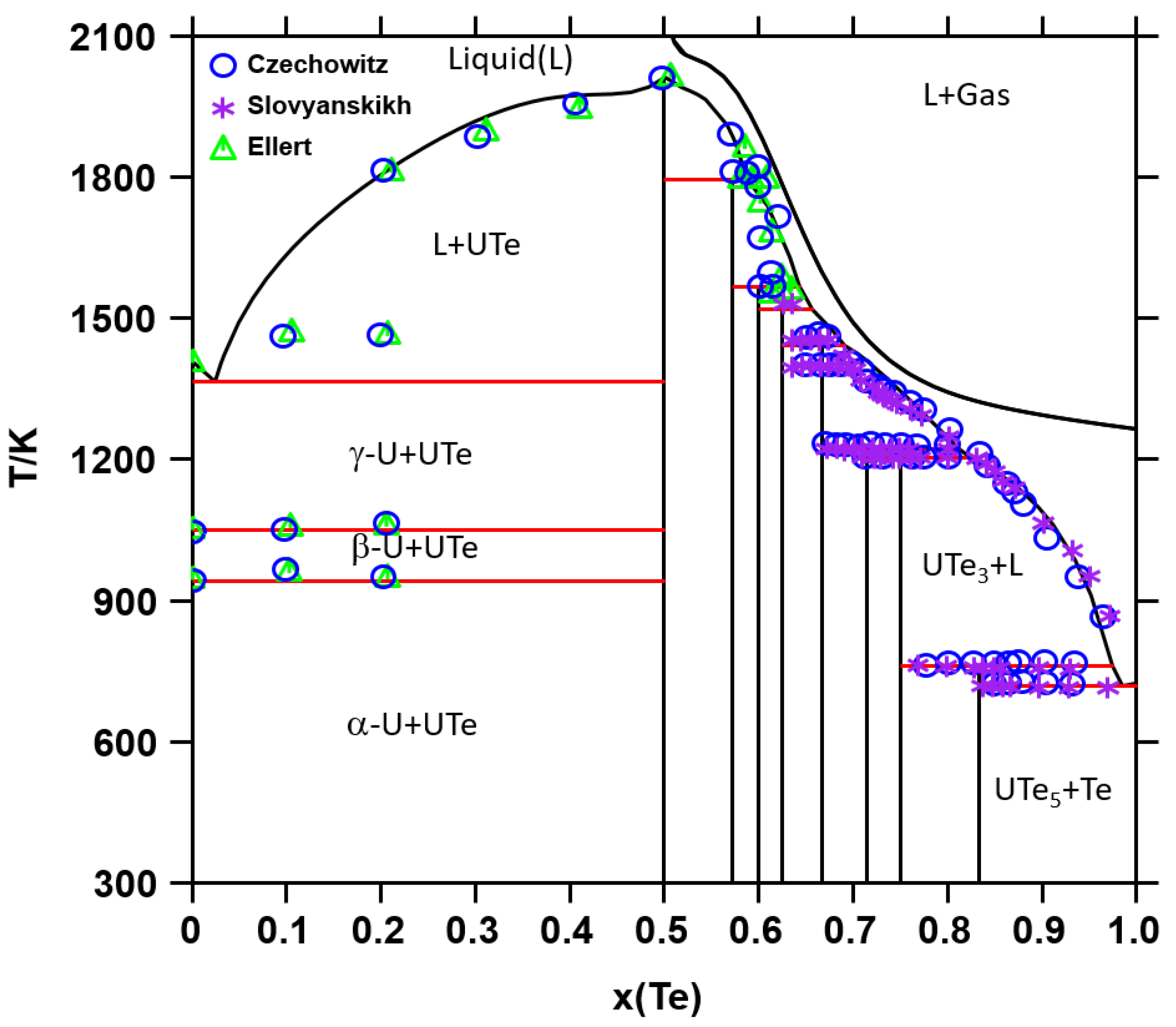
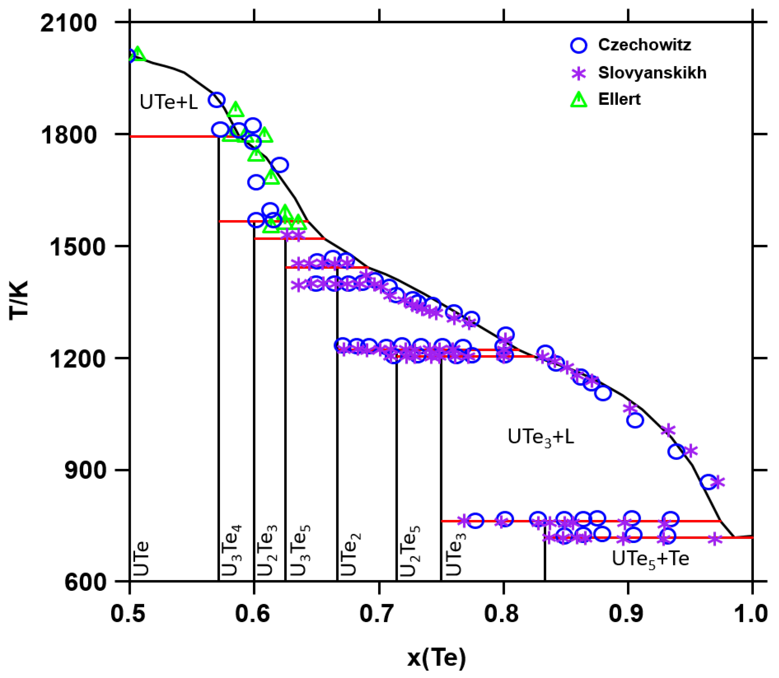
The calculated phase diagram is compared to the experimental data in Figure 2 and Figure 3. In the UTe–Te region (Figure 3), a very good agreement is obtained with the experimental data. The liquidus curve and the invariant reactions are very well reproduced from UTe${}_2$ to Te. Only the plateau related to the polymorphic transition of UTe${}_2$ was not described in the present assessment as the transition enthalpy of the compound is unknown. The liquidus curve from UTe to UTe${}_2$ and the temperature of the peritectic decomposition of U${}_3$Te${}_4$ and U${}_2$Te${}_3$ remain uncertain due to very few scattered experimental data in this region. In the U–UTe region, the experimental data are scarce so the liquidus curve shape remains quite uncertain. Moreover, the experimental eutectic temperature between U and UTe was overestimated in the measurements due to a chemical interaction between the sample and the crucible. Thus the discrepancy with the model was expected. New measurements shall be performed to improve the phase diagram knowledge in the U–UTe${}_2$ composition range.

Concerning the thermodynamic data, the enthalpy of formation and standard entropies of the compounds are calculated in Figure 4 and Figure 5, respectively.

The available data from the literature are reported for comparison. The model is in very good agreement with the experimental data of Baskin et al. [23] for U${}_3$Te${}_4$ whereas it is less good for UTe and UTe${}_2$. However, the value for UTe${}_2$ was not measured but estimated. Our calculated data are in good agreement with the data derived from the Calphad model of Wolf [20], except for UTe and U${}_3$Te${}_4$. Our data are much higher than the values coming from the Solgasmix model of Czechowitz [19]. Finally, as expected, our model is in disagreement with the DFT data which are very far from the experimental data of Baskin et al. [23]. Concerning the entropies, our model is in reasonable agreement with the estimations by Westrum [21] and the model of Wolf [20] who considered a mixing law between U and Te. New measurements of thermodynamic data for the compounds would be very useful to improve the reliability of the model.

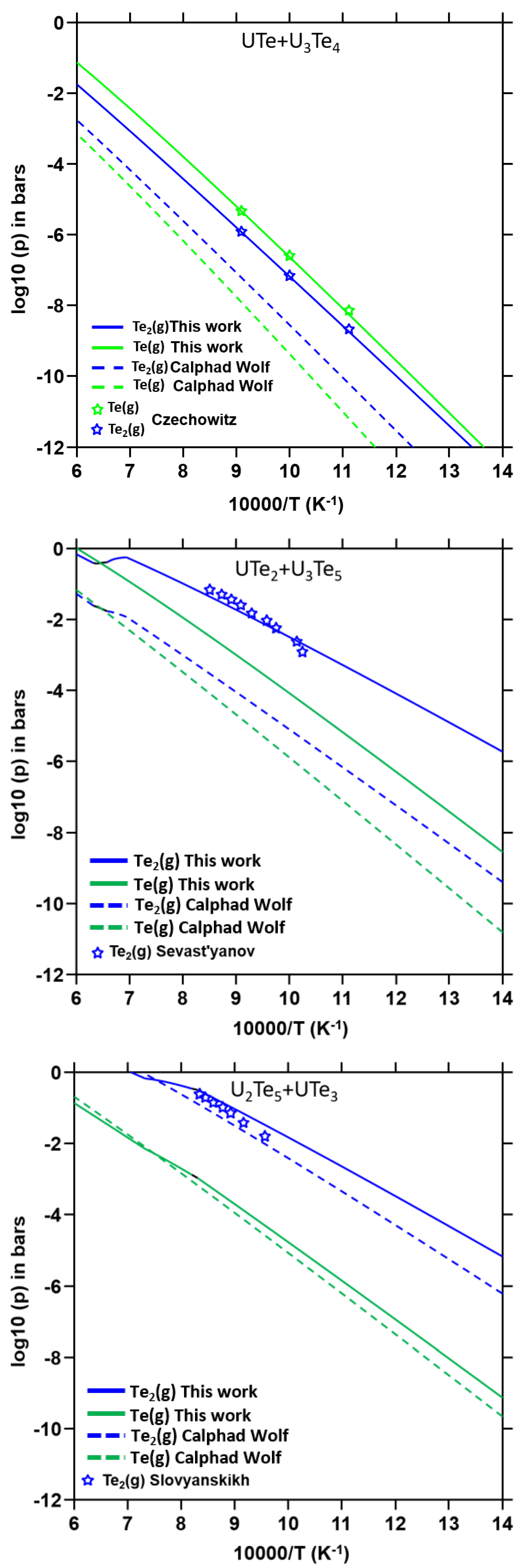
The calculated partial pressure data in the two phase regions (UTe + U${}_3$Te${}_4$), (U${}_3$Te${}_5$ + UTe${}_2$), and (U${}_2$Te${}_5$ + UTe${}_3$) are compared with the available experimental data in Figure 6. Our model is in very good agreement with the experimental data for the three two-phase regions. On the contrary, the data calculated with the model of Wolf [20] lead to a systematic underestimation of the partial pressure data.

In conclusion, the CALPHAD model reproduces most of the selected data. However, the enthalpy of the formation of UTe is underestimated. This could be due to the inconsistency between the enthalpy of formation of UTe and the partial pressure data as already pointed out by Czechowitz [22].

To improve the reliability of the model, new measurements of the following data would be useful: Te activity, mixing enthalpy of formation in the liquid, enthalpy of formation, and heat capacity data for the compounds, phase diagram data in the U–UTe${}_2$ region.

5.2. Uncertainty Propagation with the Bayesian Approach

In this section, the uncertainty propagation with the Bayesian approach is studied in the UTe–Te part of the phase diagram only, as there are too few data in the U–UTe part of the diagram to perform an uncertainty analysis. The final parameter values obtained in the assessment with PARROT as well as the posterior average and standard deviation values are reported in Table 4.

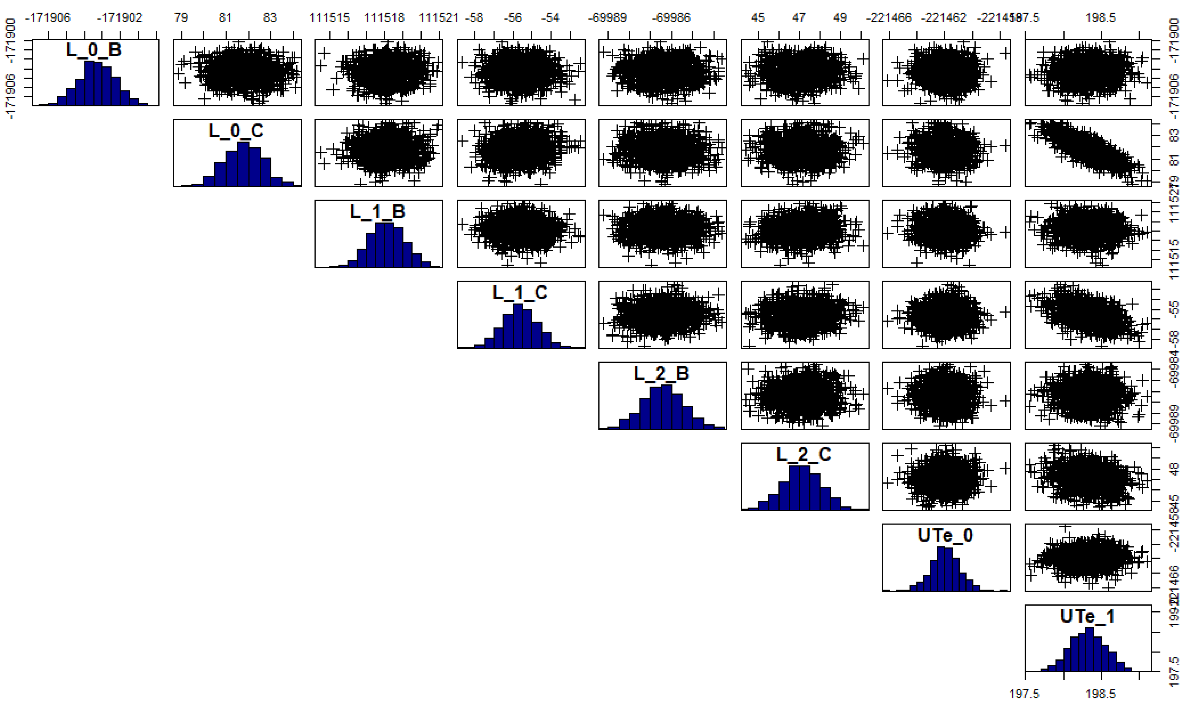
Figure 7 and Figure 8 show the plot matrices of the parameters posterior probability distribution: for the liquid phase and UTe in Figure 7 and for the solid compounds entropy parameters in Figure 8. Notice that it is possible to build such plot matrices for the whole set of parameters. However, for clarity purposes, small groups of parameters are selected. The groups selected are those showing more dependencies.

We briefly recall how to read such graphs. In Figure 8 the eight diagonal plots are the histograms of each entropy parameter. The scatterplots above the diagonal show the correlations between all parameters. For example in Figure 8, the first row gives the correlations between UTe and the other compounds. Ellipses and circular correlation scatterplots are a direct consequence of the Gaussian distribution. A thin ellipse means that there exists a strong relationship between the two parameters values. On the contrary, a circular scatterplot is the result of a low dependency.

Figure 8 shows strong correlations for the compounds that have close compositions. For example, the correlation values are above 0.97 for the pairs U${}_2$Te${}_3$–U${}_3$Te${}_5$, U${}_2$Te${}_5$–UTe${}_3$, and UTe${}_3$-UTe${}_5$. Conversely, the correlation values decrease as the compositions become more distant. The pair UTe–UTe${}_5$ has the lowest correlation value, which is below 0.01. The complete correlation matrix is given in the Appendix B.

The other parameters are not very correlated. Figure 7 shows no correlation between the liquid parameters. The only strong correlation that can be observed on this graph is the one between the parameter C for the order 0 interaction term and the entropy parameter for UTe with a correlation value slightly above −0.7.

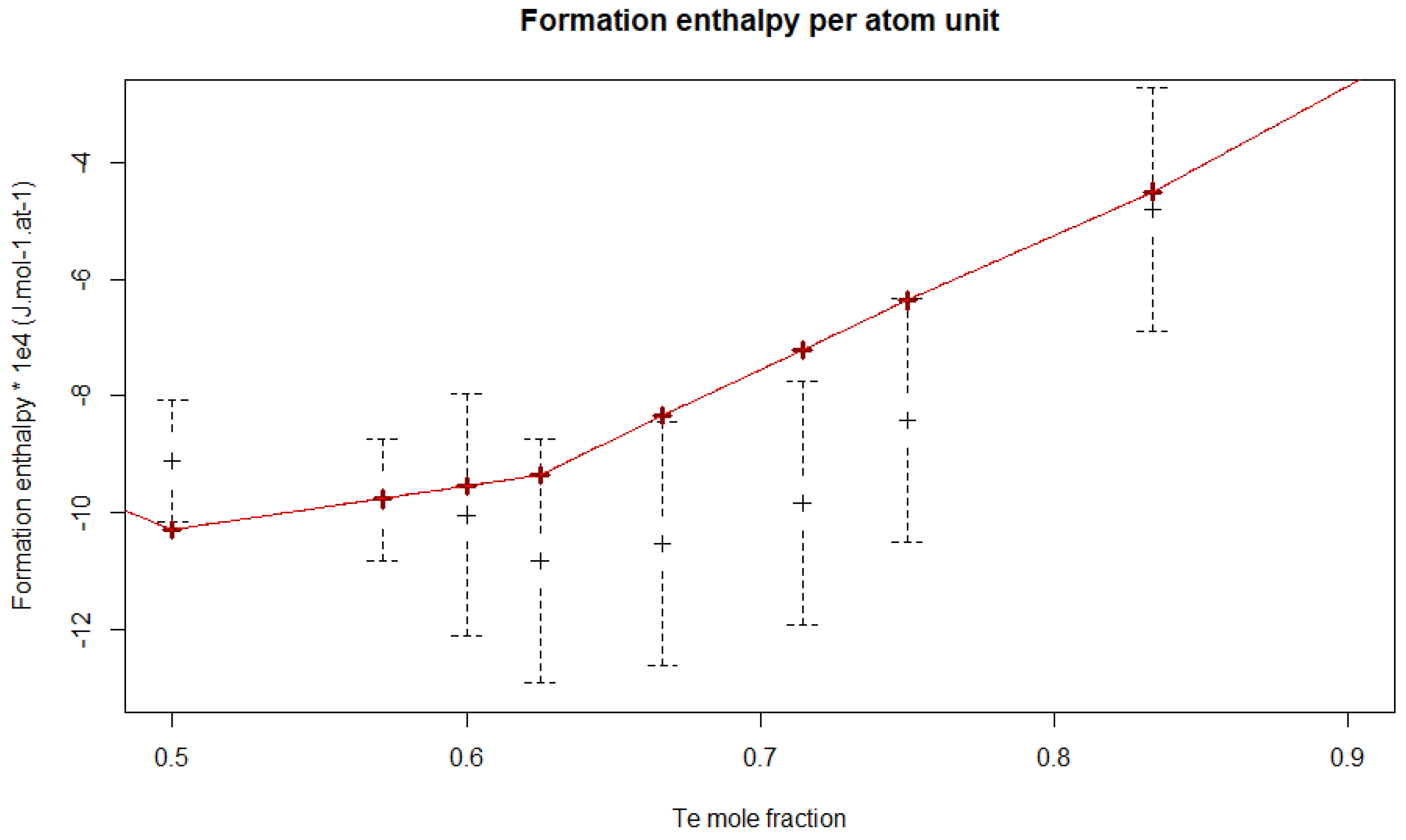
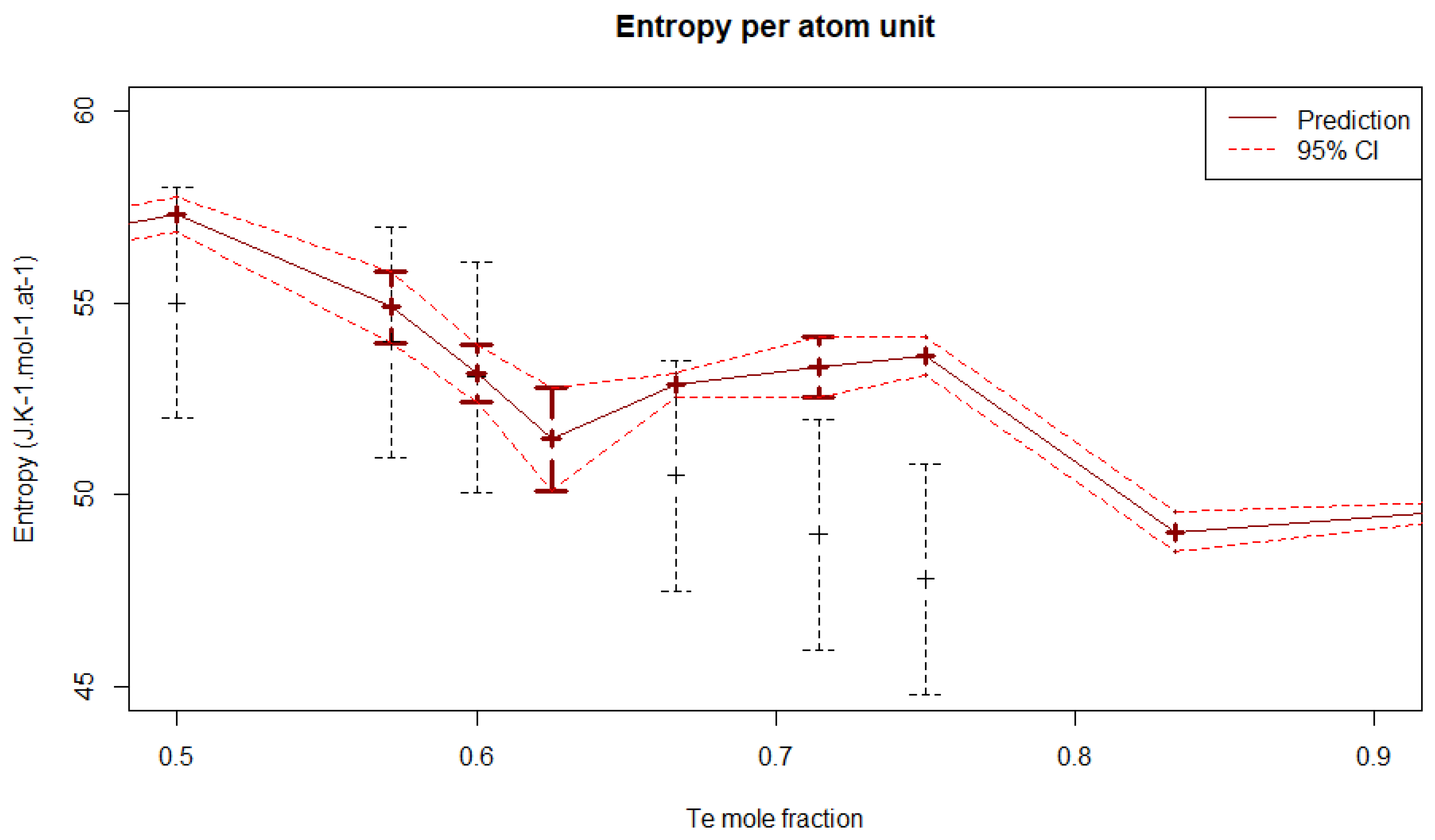
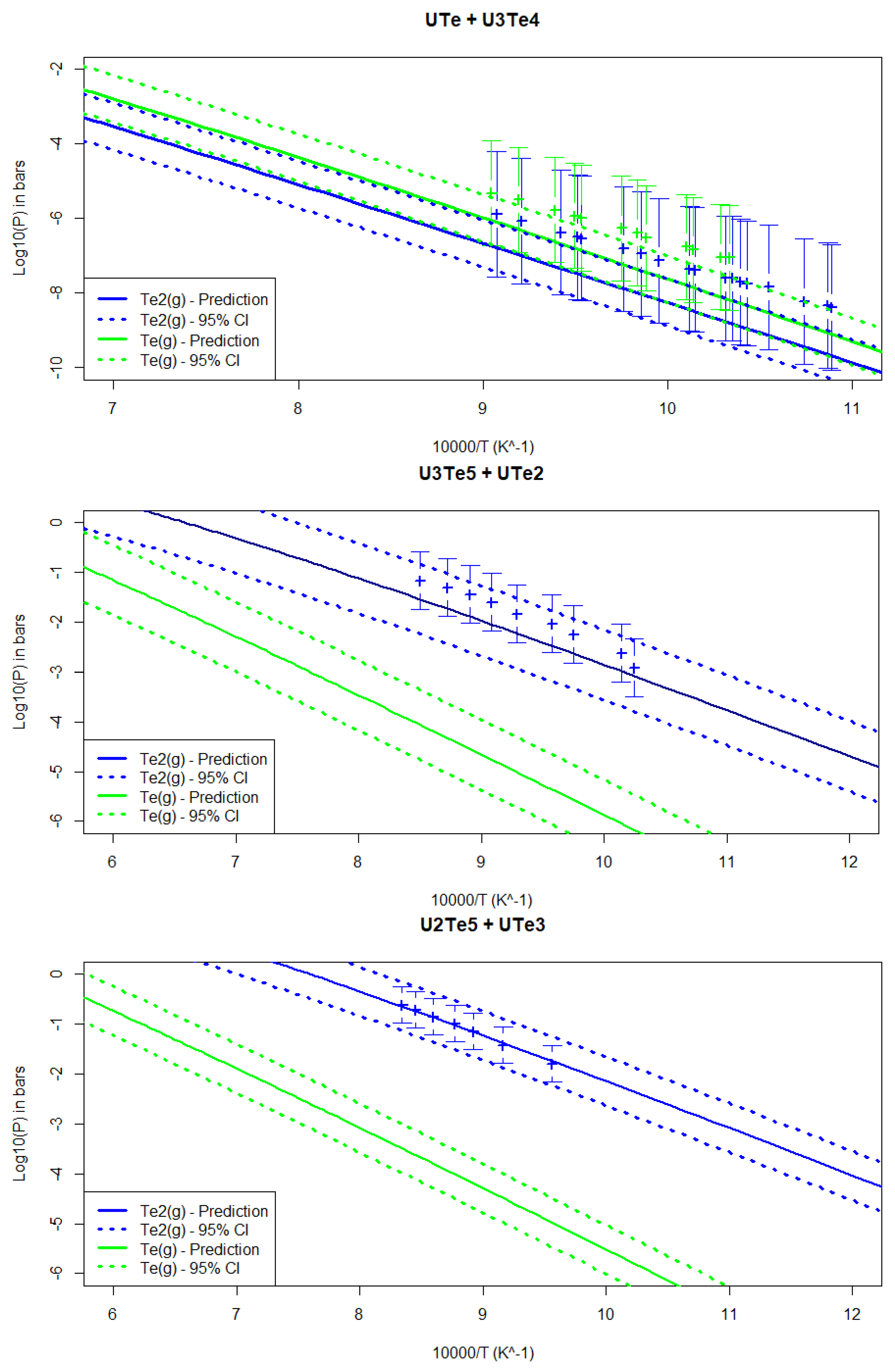
Using the methodology described in Section 4, the uncertainty of the different calculated thermodynamic quantities are compared with the experimental data in Figure 9 for $\Delta H_{f,298.15K}^0$, Figure 10 for $S_{298.15K}^0$, and Figure 11 for the partial pressure corresponding to the two-phases regions (UTe + U${}_3$Te${}_4$), (U${}_3$Te${}_5$ + UTe${}_2$), and (U${}_2$Te${}_5$ + UTe${}_3$). The prediction errors show a rather good agreement with the partial pressure data. The obtained credible intervals are in adequacy with the experimental results; circa plus or minus 0.1 bar for UTe–U${}_3$Te${}_4$ and UTe${}_2$–U${}_3$Te${}_5$, plus or minus 0.05 bar for UTe${}_3$–U${}_2$Te${}_5$. In addition, for the partial pressure in the UTe–U${}_3$Te${}_4$ region which shows the largest experimental uncertainty, the posterior credible interval length corresponds to half of the value of the experimental uncertainty. In Figure 9 and Figure 10, the obtained propagated uncertainties appear to be rather small compared to the fitting data error bars and the obtained propagated uncertainty for the partial pressure in Figure 11. Such differences could be explained by the fact that the determination of partial pressure confidence sets involves several parameters whereas the confidence sets for $\Delta H_{f,298.15K}^0$ and $S_{298.15K}^0$ depend on a single parameter. Both Figure 4 and Figure 9 show the same trend and the same strong discrepancy for the $\Delta H_{f,298.15K}^0$ value of UTe. Despite such a gap with the thermodynamic data, the assessed model is in better agreement with the phase diagram.

In Figure 10, one can observe especially small credible intervals for UTe and UTe${}_2$. This observation is contrary to the expected result as very few fitting data were used. Considering the mismatch in the experimental data of $\Delta H_{f,298.15K}^0$, $S_{298.15K}^0$ and the partial pressure, this unexpected result could be caused by inconsistent data. Meaning that it appears to be difficult to find parameters values that are in adequacy with all the fitting data.

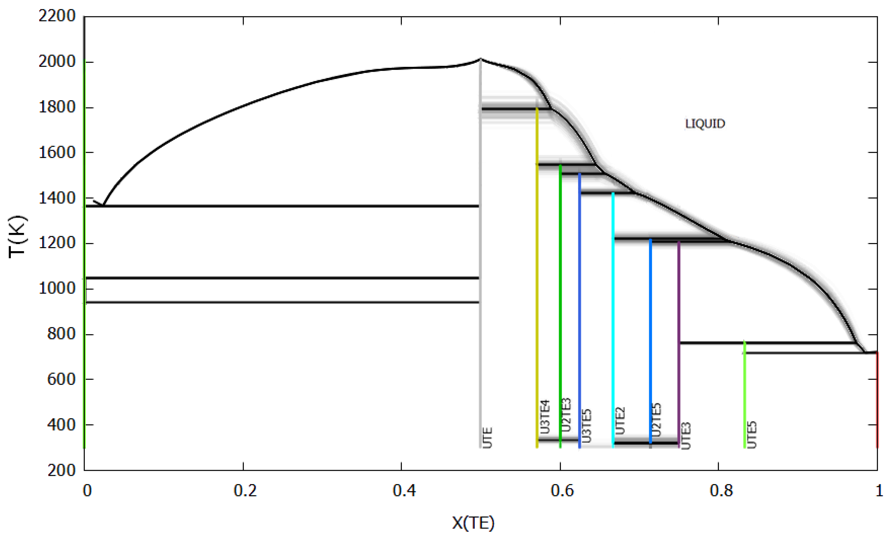
Figure 12 displays $N=100$ simulations of the phase diagram. Each phase diagram has been computed with the fifth version of the open-source software OpenCalphad [38,39]. Each simulation has been obtained by computing the phase diagram with a sample drawn from the posterior probability distribution of the whole set of parameters. Despite the small posterior uncertainty of the thermodynamic data, large posterior uncertainty can be observed on the right side of the diagram for the liquidus curve and the melting temperatures of U${}_3$Te${}_4$, U${}_2$Te${}_3$, U${}_3$Te${}_5$, U${}_2$Te${}_5$, and UTe${}_3$. The estimated uncertainty for the melting temperature of U${}_2$Te${}_3$, U${}_3$Te${}_5$, U${}_2$Te${}_5$, and UTe${}_3$ is around 50 K and 100 K for the melting temperature of U${}_3$Te${}_4$.

Notice that, for some parameters values drawn from the posterior probability distribution, the compounds U${}_2$Te${}_3$, UTe${}_2$, and U${}_2$Te${}_5$ may not be stable at 298.15 K. Such results lead to the existence of an invariant transition below 350 K for these compounds. In the phase diagrams found in the literature, these compounds are assumed to be stable at room temperature [9,13,18,19]. However, more enthalpy of formation data are required to confirm this assumption. Moreover, these compounds have very close compositions, and even small variation of parameters values can lead to unstable compounds at room temperature.

6. Conclusions

In a first step, the thermodynamic assessment of the uranium–tellurium system has been performed using the CALPHAD method. Experimental phase diagram and thermodynamic data have been used as input data to optimize the Gibbs energy functions for UTe, U${}_3$Te${}_4$, U${}_2$Te${}_3$, U${}_3$Te${}_5$, UTe${}_2$, U${}_2$Te${}_5$, UTe${}_3$, and UTe${}_5$ and for the liquid phase.

It should be noted that there do not exist any thermodynamic data on the liquid phase. Moreover, for the compounds, measurements of enthalpy of formation data at 298 K are only available for UTe and U${}_3$Te${}_4$, for which large error bars were assigned due to the large uncertainties in the measurements. Only estimations exist for the other compounds and all the enthalpy data show very large discrepancies. Unfortunately, the DFT calculations, which are very tricky on uranium tellurium compounds, did not help to make a choice as the results are far from the few experimental existing data.

For the standard entropy data at 298 K, only estimations are available. Due to the absence of experimental data, the Kopp–Neumann law was used for the heat capacity function for the compounds. The only other experimental data available are vapor pressure measurements in two phase regions: UTe–U${}_3$Te${}_4$, UTe${}_2$–U${}_3$Te${}_5$, and U${}_2$Te${}_5$–UTe${}_3$. Input thermodynamic data for the model were carefully selected. The phase diagram from pure U to UTe${}_2$ is quite uncertain. In fact, only a few liquidus data were measured. On the contrary, the phase diagram is very well established from UTe${}_2$ to pure Te.

The CALPHAD model reproduces very well the experimental vapor pressure data and enthalpy of formation for U${}_3$Te${}_4$. However, the calculated enthalpy of formation for UTe is underestimated by 13% compared to the measured value. The agreement with Westrum estimations for the entropies of U${}_3$Te${}_4$ and U${}_2$Te${}_3$ is very good. Higher values are obtained for the other compounds with deviations from 5% (for UTe, UTe${}_2$) to 12% for UTe${}_3$. The calculated phase diagram is in very good agreement with the experimental data. For comparison, the CALPHAD model of Wolf leads to a very good agreement with the enthalpy of formation for UTe whereas it overestimates the enthalpy for U${}_3$Te${}_4$. Moreover, it tends to underestimate systematically the vapor pressure data and the liquidus curve are not well reproduced compared to the experimental points. It clearly shows that in both CALPHAD assessments, it was finally not possible to get a good agreement with all the experimental data. One of the reasons is the inconsistency between the experimental enthalpy of formation data and the vapor pressure measurements.

In a second step, the uncertainty analysis was performed on the CALPHAD model. The prediction error shows a good agreement with the partial pressure experimental uncertainty and small confidence intervals. The prediction model shows more discrepancies with the entropy data and the enthalpy of formation data. The prediction error however remains very small (less than 0.1%) for the enthalpy of formation and quite small (between 1% and 4%) for the entropy.

Despite the global little uncertainty on the predicted thermodynamic data, one can observe rather large estimated uncertainty on the phase diagram. In particular the estimated uncertainty for the melting temperature of U${}_3$Te${}_4$ is around 100 K.

From a global perspective, the whole system lacks a sufficient amount of fitting data. The system complexity and the number of parameters are too important for the too few numbers of fitting data (120 points versus 22 parameters) and we do not have any thermodynamic data on the liquid. New experimental data, like heat capacity, enthalpy of formation measurements for the different compounds, and chemical potential values for the liquid phase could improve the model.

Given our results, we have little confidence in the assessed model and recommend additional measurements to improve the knowledge on the UTe–Te side of the system.

From a wider perspective, we renew with this study the advantages of the conjugate prior approach. Contrary to other Bayesian methods, such an approach allows us to have an analytical posterior probability distribution and, therefore, closed-form expressions for the uncertainty of the calculated thermodynamic quantities. Having an analytical posterior probability distribution also speeds up the simulation of the system parameters which makes easier the study of the uncertainty propagation to the phase diagram. In further work, we will apply this methodology to the study of a ternary system and to the propagation of the system parameters uncertainty when coupling with a multi-physics code.

References

1. Samuelsson, K.; Dumas, J.C.; Sundman, B.; Lainet, M. An improved method to evaluate the “Joint Oxyde-Gaine” formation in (U,Pu)O2 irradiated fuels using the GERMINAL V2 code coupled to Calphad thermodynamic computations. EPJ Nucl. Sci. Technol. 2020, 6, 47. [Google Scholar] [CrossRef]
2. Samuelsson, K.; Dumas, J.C.; Sundman, B.; Lamontagne, J.; Guéneau, C. Simulation of the chemical state of high burnup (U,Pu)O2 fuel in fast reactors based on thermodynamic calculations. J. Nucl. Mater. 2020, 532, 151969. [Google Scholar] [CrossRef]
3. Guéneau, C.; Dupin, N.; Kjellqvist, L.; Geiger, E.; Kurata, M.; Gossé, S.; Corcoran, E.; Quaini, A.; Hania, R.; Smith, A.L.; et al. TAF-ID: An international thermodynamic database for nuclear fuels applications. Calphad 2021, 72, 102212. [Google Scholar] [CrossRef]
4. Lukas, H.L.; Fries, S.G.; Sundman, B. Computational Thermodynamics: The Calphad Method; Cambridge University Press: Cambridge, UK, 2007. [Google Scholar]
5. Paulson, N.H.; Bocklund, B.J.; Otis, R.A.; Liu, Z.-K.; Stan, M. Quantified uncertainty in thermodynamic modeling for materials design. Acta Mater. 2019, 174, 9–15. [Google Scholar] [CrossRef] [Green Version]
6. Paulson, N.H.; Jennings, E.; Stan, M. Bayesian strategies for uncertainty quantification of the thermodynamic properties of materials. Int. J. Eng. Sci. 2019, 142, 74–93. [Google Scholar] [CrossRef] [Green Version]
7. Paulson, N.H.; Zomorodpoosh, S.; Roslyakova, I.; Stan, M. Comparison of statistically-based methods for automated weighting of experimental data in CALPHAD-type assessment. Calphad 2020, 68, 101728. [Google Scholar] [CrossRef]
8. Thermo-Calc Software, Version 2021a. Available online: https://thermocalc.com/ (accessed on 15 January 2021).
9. Okamoto, H. Te-U (Tellurium-Uranium). J. Phase Equilibria 1993, 14, 129–130. [Google Scholar] [CrossRef]
10. Herrmannsdörfer, T.; Fischer, P.; Mattenberger, K.; Vogt, O. Temperature dependences of rhombohedral lattice distortion and of ferromagnetic uranium ordering in the uranium monochalcogenides. J. Alloys Compd. 2006, 414, 14–19. [Google Scholar] [CrossRef]
11. Tougait, O.; André, G.; Bourée, F.; Noël, H. Neutron diffraction study of magnetic ordering of two binary uranium tellurides U3Te5 and U2Te3. J. Alloys Compd. 2001, 317–318, 227–232. [Google Scholar] [CrossRef]
12. Stöwe, K. Contributions to the Crystal Chemistry of Uranium Tellurides. III. Temperature-Dependent Structural Investigations on Uranium Ditelluride. J. Solid State Chem. 1996, 127, 202–210. [Google Scholar] [CrossRef]
13. Solvyanskikh, V.K.; Yarembash, E.I.; Ellert, G.V.; Eliseev, A.A. On the system U-Te. Izv. Akad. SSSR Ser. Neor. Materialy 1968, 4, 543–545. [Google Scholar]
14. Solvyanskikh, V.K.; Rozanov, I.A.; Gracheva, N.V. The S-Te-U. Russ. J. Inorg. Chem. 1977, 22, 893–896. [Google Scholar]
15. Tougait, O.; Potel, M.; Noël, H. Characterization of the Binary Uranium and Thorium Tellurides U7Te12 and Th7Te12. Inorg. Chem. 1998, 37, 5088–5091. [Google Scholar] [CrossRef]
16. Tougait, O.; Potel, M.; Padiou, J.; Noël, H. Crystal structure and properties of the binary uranium telluride U2Te5. J. Alloys Compd. 1997, 262–263, 320–324. [Google Scholar] [CrossRef]
17. Boehme, D.R.; Nichols, M.C.; Snyder, R.L.; Matheis, D.P. An investigation of the tellutium-rich uranium tellurides using X-ray powder diffraction. J. Alloys Compd. 1992, 179, 37–59. [Google Scholar] [CrossRef]
18. Ellert, G.V.; Sevast’yanov, V.G.; Solvyanskikh, V.K. The Se-U and Te-U Systems. Russ. J. Inorg. Chem. 1975, 20, 120–124. [Google Scholar]
19. Czechowicz, D.G. Combustion Synthesis and Characterization of Uranium and Thorium Tellurides: LA-10559-T. Master’s Thesis, Los Alamos National Laboratory, Los Alamos, NM, USA, 1985. [Google Scholar]
20. Wolf, A. Modellierungen zur Kristallzüchtung von CrSb2 und UPTe, Ein Beitrag zur Rationale Syntheseplanung; Springer: Wiesbaden, Germany, 2017. [Google Scholar] [CrossRef]
21. Westrum, E.F.; Gronvold, F. Chemical Thermodynamics of the Actinide Element Chalcogenides. In Proceedings of the Symposium on Thermodynamics of Nuclear Materials (IAEA), Vienna, Austria, 21–25 May 1962. [Google Scholar]
22. Czechowicz, D.G. A Study of vaporization Thermodynamics in the Uranium-Tellurium System: LA-10621-T. Master’s Thesis, Los Alamos National Laboratory, Los Alamos, NM, USA, 1986. [Google Scholar]
23. Baskin, Y.; Smith, S.D. Enthalpy of formation data on compounds of uranium with groups VA and VIA elements. J. Nucl. Mater. 1970, 37, 209–222. [Google Scholar] [CrossRef]
24. Mills, K.C. Thermodynamic Data for Inorganic Sulphides, Selenides and Tellurides; Butterworth & Co.: London, UK, 1974. [Google Scholar]
25. Qian, S.; Qiu, R.; Tang, J.; Chen, J.; Liu, P.; Ao, B. Theoretical Assignment of Oxidation State of Uranium in Binary, Ternary, and Quaternary Tellurides. J. Phys. Chem. 2021, 125, 1029–1040. [Google Scholar] [CrossRef]
26. Saal, J.E.; Kirklin, S.; Aykol, M.; Meredig, B.; Wolverton, C. Materials Design and Discovery with High-Throughput Density Functional Theory: The Open Quantum Materials Database (OQMD). JOM 2013, 65, 1501–1509. [Google Scholar] [CrossRef]
27. Solvyanskikh, V.K.; Ellert, G.V.; Yarembash, E.S. Transport mechanism and kinetics in Uranium chalcogenides. Izv. Akad. SSSR Ser. Neor. Mater. 1967, 3, 1133. [Google Scholar]
28. Sevast’yanov, V.G.; Solvyanskikh, V.K.; Ellert, G.V. Equilibria in the USx–Br2 and USex–Br2 system. Zh. Neorg. Khim. 1971, 16, 3357. [Google Scholar]
29. Dinsdale, A.T. SGTE data for pure elements. Calphad 1991, 15, 317–425. [Google Scholar] [CrossRef]
30. Hillert, M.; Jansson, B.; Sundman, B.; Agren, J. A two-sublattice model for molten solutions with different tendency for ionization. Metall. Trans. 1985, 16, 661. [Google Scholar] [CrossRef]
31. SSUB5: SGTE Substances Database, Version 5.2. Available online: https://thermocalc.com/products/databases/general-alloys-and-pure-substances/ (accessed on 15 January 2016).
32. Guillaumont, R. Update on the Chemical Thermodynamics of Uranium, Neptunium, Plutonium, Americium and Technetium; OECD Nuclear Energy Agency, Data Bank: Issy-les-Moulineaux, France, 2003. [Google Scholar]
33. Chatterjee, N.D.; Krüger, R.; Haller, G.; Olbricht, W. The bayesian approach to an internally consistent thermodynamic database: Theory, database, and generation of phasediagrams. Contrib. Mineral. Petrol. 1998, 133, 149–168. [Google Scholar] [CrossRef]
34. Duong, T.C.; Hackenberg, R.E.; Landa, A.; Honarmandi, P.; Talapatra, A.; Volz, H.M.; Llobet, A.; Smith, A.I.; King, G.; Bajaj, S.; et al. Revisiting thermodynamics and kinetic diffusivities of uranium–niobium with bayesian uncertainty analysis. Calphad 2016, 55, 219–230. [Google Scholar] [CrossRef] [Green Version]
35. Lawrence, E. Reconstruction Fonctionnelle et Analyse D’incertitude dans le Cadre d’un Problème Inverse de Thermodynamique Chimique. Ph.D. Thesis, Université Paul Sabatier Toulouse 3, Toulouse, France, 2020. [Google Scholar]
36. Robert, C.P. The Bayesian Choice: A Decision-Theoretic Motivation; Springer: New York, NY, USA, 1994. [Google Scholar]
37. Azaïs, J.M.; Bardet, J.M. Le Modèle Linéaire par L’exemple. Régression, Analyse de la Variance et Plans d’Expériences. Illustrations Numériques avec les Logiciels R, SAS et Splus; Dunod: Paris, France, 2006. [Google Scholar]
38. Sundman, B.; Lu, X.G.; Ohtani, H. The implementation of an algorithm to calculate thermodynamic equilibria for multi-component systems with non-ideal phases in a free software. Comput. Mater. Sci. 2015, 101, 127–137. [Google Scholar] [CrossRef]
39. The OpenCalphad Repository. Available online: http://github.com/sundmanbo/opencalphad (accessed on 12 December 2018).
Figure 1. Enthalpy of formation data of the U x Te y compounds coming from the literature. The uncertainty bars on the experimental data measured by calorimetry (in blue) are reported.
Thermo 02 00003 g001
Figure 2. Calculated phase diagram. Comparison with the experimental data from Czechowitz [19], Slovyanskikh et al. [13] and Ellert et al. [18].
Thermo 02 00003 g002
Figure 3. Calculated phase diagram from 50 to 100 at. % Te. Comparison with the experimental data from Czechowitz [19], Slovyanskikh et al. [13] and Ellert et al. [18].
Thermo 02 00003 g003
Figure 4. Calculated enthalpy of formation of UTe, U 3 Te 4 , U 2 Te 3 , U 3 Te 5 , UTe 2 , U 2 Te 5 , UTe 3 , and UTe 5 . Comparison with the experimental data from Baskin et al. [23], the models from Czechowitz [19] and Wolf [20], and the DFT calculations from Qian [25] and the OQMD database [26].
Thermo 02 00003 g004
Figure 5. Calculated standard entropy at 298.15 K of UTe, U 3 Te 4 , U 2 Te 3 , UTe 2 , U 2 Te 5 , and UTe 3 . Comparison with the estimated data from Westrum [21] and the model of Wolf [20].
Thermo 02 00003 g005
Figure 6. Calculated partial pressure of Te and Te 2 in (UTe + U 3 Te 4 ), (U 3 Te 5 + UTe 2 ), and (U 2 Te 5 + UTe 3 ) in plain lines. Comparison with the experimental results in [22,27,28], and the model of Wolf [20] in dotted lines.
Thermo 02 00003 g006
Figure 7. Parameter posterior probability distributions and correlations matrix plot for the liquid phase on UTe–Te side and UTe. The posterior correlation values can be found in Appendix B.
Thermo 02 00003 g007
Figure 8. Parameter posterior probability distributions and correlations matrix plot for the compounds entropic parameters. The posterior correlation values can be found in Appendix B.
Thermo 02 00003 g008
Figure 9. Uncertainty estimation given by the 95% credible interval of the posterior probability distribution for the calculated enthalpies of formation for UTe, U 3 Te 4 , U 2 Te 3 , U 3 Te 5 , UTe 2 , U 2 Te 5 , UTe 3 , and UTe 5 . The experimental error bars are in dotted black lines. The propagated uncertainties (95% credible interval) for each computed quantity are in bold red lines.
Thermo 02 00003 g009
Figure 10. Uncertainty estimation given by the 95% credible interval of the posterior probability distribution for the calculated entropies for UTe, U 3 Te 4 , U 2 Te 3 , UTe 2 , U 2 Te 5 , and UTe 3 . The experimental error bars are in doted black lines. The propagated uncertainties (95% credible interval) for each computed quantity are in bold red lines.
Thermo 02 00003 g010
Figure 11. Uncertainty estimation given by the 95% credible interval of the posterior probability distribution for the calculated partial pressure. Plain lines are the posterior means. Dotted lines correspond to the 95% upper and lower bounds of the credible interval for each temperature value.
Thermo 02 00003 g011
Figure 12. Simulation of N = 100 phase diagram from the parameters posterior probability distribution.
Thermo 02 00003 g012