Fast and Interpretable Estimation of Amino Acid Residue Surface Accessibility Based on Protein Contact Graph

Abstract

The solvent-accessible surface area (SASA) of amino acid residues is a crucial parameter for protein structure analysis; however, precise computational methods such as FreeSASA are computationally expensive. As an alternative, empirical approximations based on residue interaction network (RIN) graphs can offer high speed while maintaining acceptable accuracy. In this study, we propose and validate three empirical functions for estimating relative SASA—approx_sasa, surface_score, and exp_sasa—using node degree as the sole argument. We present a comparative analysis of two graph construction approaches: the classical Cα-graph (8 Å threshold) and the heavy-atom graph (HAG, 5.0 Å threshold). Parameters were calibrated on a dataset of 509 protein structures (128,794 residues) using the true relative SASA calculated by the FreeSASA library. An extended set of 11 topological features was also developed and validated. Ensemble models (Random Forest, XGBoost) achieved a best performance of MAE = 0.057 ± 0.033 and Pearson r = 0.915 ± 0.080 on HAG, outperforming graph neural networks (GCN, GAT, GraphSAGE) in this setting. The empirical formulas demonstrate extreme computational efficiency (0.008 ms per structure), ~26,000× faster than FreeSASA, making them suitable for large-scale pipelines requiring both speed and interpretability. Random Forest on HAG is recommended for applications requiring maximum accuracy, while GraphSAGE on HAG is a viable deep learning alternative.

1. Introduction

The solvent-accessible surface area (SASA) of amino acid residues is a fundamental property in protein structure analysis, widely employed for identifying surface residues, predicting binding sites and epitopes, and evaluating protein packing quality [1,2]. Conventional SASA calculation methods, such as the Shrake–Rupley algorithm [3], as implemented in DSSP [4] or FreeSASA [5], require full three-dimensional atomic-resolution protein geometries. These approaches are computationally expensive for large-scale applications, including virtual screening and training machine learning models on thousands of PDB structures.

A practical alternative involves empirical functions based on simple graph characteristics, such as node degree in the residue interaction network (RIN). RINs are typically constructed from Cα-Cα distances, where node degree reflects the number of spatial neighbors of a residue—a property closely linked to packing density and inversely correlated with solvent accessibility [6]. While the correlation between RIN node degrees and SASA values is well-recognized, its practical application requires careful quantification and parameter selection. Here, we investigate two contact graph construction strategies and systematically evaluate their suitability for SASA prediction.

The first approach is a classical Cα-graph with an 8 Å cutoff, where each residue is represented by its Cα atom coordinates, and edges are added when the Cα-Cα distance is <8 Å. This method offers minimal computational overhead and is widely adopted in the literature [6].

The second approach employs a heavy-atom graph (HAG) with a 5.0 Å cutoff. Here, each residue is represented by the coordinates of all its heavy atoms (C, N, O, S, etc., excluding hydrogens), and edges are added if the minimum distance between any heavy atoms from two residues is <5.0 Å.

For each graph type, we propose and validate three empirical features for estimating a relative SASA: approx_sasa (linear saturation model), surface_score (piecewise linear function), and exp_sasa (exponential model). Formal parameter optimization was performed on an extended dataset of 509 protein structures from the PDB, with a resolution of ≤2.0 Å and an R-factor ≤ 0.25. This ensures statistical reliability and enables assessment of model generalization across diverse protein folds.

We also explore an extended set of 11 topological features derived from the RIN, comprising basic node properties, centrality measures (betweenness, eigenvector, and closeness), and hydrophobic subgraph attributes. Ensemble models (Random Forest and XGBoost) trained on these features using the Leave-One-Structure-Out (LOSO) cross-validation scheme enable precise quantification of the accuracy gains over the empirical formulas.

We compared our approach with graph neural networks (GCN, GAT, and GraphSAGE). These models were trained using a 70/15/15 train/validation/test split with early stopping and hyperparameter optimization.

Building on previous graph-based SASA studies [6], our work makes three key contributions. First, we systematically compare two fundamentally different graph representations—the classical Cα-graph and the heavy-atom graph (HAG)—providing a comprehensive analysis of their impact on SASA prediction accuracy. Second, we propose and validate a unified framework of three interpretable empirical functions that rely solely on the node degree, offering a combination of speed and interpretability. Third, we provide a large-scale benchmark of machine learning models and graph neural networks on a diverse dataset of 509 structures, establishing clear practical guidelines for method selection based on specific task requirements.

The accurate determination of the SASA has motivated the development of various computational tools and algorithms. Ali et al. [7] provided a comprehensive review of methods for estimating the SASA in both folded and unfolded proteins, covering classical geometric approaches and their approximations. The widely used NACCESS program [8] implements the Lee–Richards algorithm for calculating atomic and residue SASAs. More recently, Ribeiro et al. [9] introduced dr_sasa, a tool for calculating accurate interatomic contact surface areas. Teruel et al. [10] developed the Surfaces software for quantifying and visualizing interactions within and between proteins and ligands. Ma et al. [11] developed ARIP, a tool for precise interatomic contact-area and contact-volume calculations, using a contact-area calculation approach derived from dr_sasa, with applications for residue packing and interface analyses. Additionally, Cao et al. [12] presented dSASA, an exact analytical and differentiable GPU-accelerated method for SASA calculations with derivatives with respect to atomic coordinates, which are particularly relevant for implicit-solvent molecular dynamics simulations and structure optimization. These tools highlight the ongoing importance of accurate SASA estimation in structural biology.

Machine learning methods, including neural networks and ensemble models, have been increasingly applied to predict various protein properties [13,14,15,16,17,18,19,20,21,22]. Recent advances have further demonstrated the power of graph neural networks and protein language models for direct SASA prediction from three-dimensional structures and sequences [23,24,25,26,27], while SASA has also been successfully integrated as a predictive feature in related tasks such as protein interaction site prediction [28] and protein stability analysis [29].

However, these approaches often demand substantial computational resources and remain “black boxes,” limiting their interpretability. In contrast, our work focuses on simple, interpretable empirical formulas that rely solely on the node degree in the contact graph, while also comparing them against more complex regression models using an extended set of topological features. We demonstrate that these simple formulas achieve high accuracy with minimal computational overhead and that their parameters can be universally calibrated on a diverse protein dataset. This comparative evaluation of ML methods and graph types provides a systematic framework for assessing trade-offs, guiding practical tool selection in structural bioinformatics.

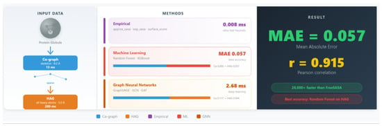
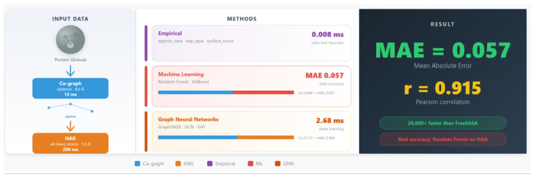
For the Cα-graph, optimal empirical formula parameters yielded a Pearson correlation of r = 0.711 with a mean absolute error (MAE) of 0.117. In contrast, the HAG-based empirical formulas achieved substantially better performance, with r = 0.813 and MAE = 0.094. The best overall results were obtained with Random Forest on HAG, which attained r = 0.915 and MAE = 0.057, corresponding to a 39% improvement over the best Cα-graph empirical formula (MAE = 0.117) and a 13% improvement over Random Forest on the Cα-graph (MAE = 0.066). GraphSAGE on HAG delivered comparable performance (MAE = 0.0715, r = 0.8917), highlighting the potential of graph neural networks when applied to HAG, whereas GCN and GAT performed considerably worse (MAE = 0.14–0.15, r = 0.51–0.61). In terms of computational efficiency, the empirical formulas required only 0.008 ms per structure (~26,000× faster than FreeSASA), while Random Forest inference took 36.5 ms (~6× faster than FreeSASA). Notably, HAG construction was 21 times more time-consuming than Cα-graph construction.

2. Materials and Methods

2.1. Data

For model validation, we used a dataset of 506 protein structures retrieved from the Protein Data Bank (PDB), all with a resolution of ≤2.0 Å and an R-factor of ≤0.25 (with a small number of exceptions). To ensure dataset diversity, we selected structures spanning a wide range of sequence lengths (from 30 to over 1000 residues; mean = 254 ± 144, median = 220) and structural classes, including α/β, α + β, all-α, and all-β proteins. The dataset resolution ranges from 0.89 to 4.62 Å (mean = 1.78 ± 0.34 Å, median = 1.80 Å). No sequence identity cutoff was applied, as our primary goal was to assess generalization across structurally diverse proteins rather than to avoid redundancy for homology-based inference. The dataset encompasses proteins from diverse sources, including viral proteins (6.3%), enzymes (54.3%), immunoglobulins (0.6%), and other protein classes (38.7%). In total, 128,751 amino acid residues were processed. For each structure, both types of contact graphs (Cα-graph and HAG) were constructed, followed by calculation of node degrees and the extended set of topological features. Ground-truth relative SASA values were computed using the FreeSASA library [5] and subsequently normalized using maximum SASA values for each amino acid type [30].

2.2. Construction of Protein Contact Graphs (RINs)

Let protein consist of amino acid residues.

2.2.1. Cα-Graph (Threshold 8 Å)

In the Cα-graph, each residue is represented by the coordinates of its Cα atom. The undirected contact graph $G_{\mathrm{C}\mathrm{a}}=(V,E)$ consists of a set of vertices $V=\{1,2,\dots N\}$, with each corresponding to a residue, and a set of edges defined by:

$$E=\{\left(i,j\right)\mid \parallel {\mathbf{r}}_i-{\mathbf{r}}_j\parallel < d_{\mathrm{cutoff}}, i\ne j\},$$

(1)

with a threshold distance $d_{\mathrm{cutoff}}=8 \AA$. The 8 Å threshold is based on typical Cα-Cα contact distances corresponding to secondary structure packing [6].

• The node degree of residue $i$ is defined as:

$$\mathrm{deg}\left(i\right)=\mid \left\{j∣\left(i,j\right)\in E\right\}.$$

(2)

This quantity reflects the number of spatial neighbors of the residue, which is inversely correlated with solvent accessibility.

2.2.2. HAG (Threshold 5.0 Å)

In contrast to the Cα-graph, the HAG represents each residue by the set of coordinates of all its heavy atoms $A_i$ (i.e., C, N, O, S, etc., excluding hydrogens), extracted directly from PDB files. An edge between two residues is added if the minimum distance between any heavy atoms of these residues is <5.0 Å:

$$E=\{\left(i,j\right)\mid \underset{a\in A_i, b\in A_j}{\mathrm{m}\mathrm{i}\mathrm{n}}\parallel {\mathbf{r}}_a-{\mathbf{r}}_b\parallel < 5.0 \AA \}.$$

(3)

The 5.0 Å cutoff is selected to capture contacts beyond the typical van der Waals range (~3.4–4.5 Å) while remaining sensitive to residue-level packing interactions.

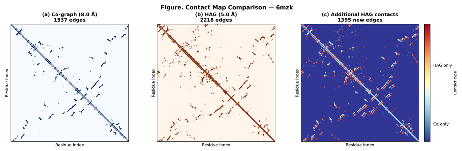
The difference in graph density between the Cα-graph and HAG is illustrated in Figure 1, which shows contact maps for a representative structure (6 mzk, 476 residues). The Cα-graph contains 1537 contacts, while HAG captures 2218 contacts—a 44% increase—with 1395 contacts (91% more than Cα) arising from side-chain and heavy-atom interactions not captured by the Cα representation. This increase in connectivity reflects the richer information captured by HAG for characterizing residue packing and solvent accessibility.

2.3. Empirical Features

The same three empirical formulas are applied to both graph types, with parameters calibrated independently for the Cα-graph and HAG.

2.3.1. Approx Sasa

Linear saturation model:

$${\widehat{s}}_i=1-\min \left({\displaystyle \frac{\mathrm{d}\mathrm{e}\mathrm{g}\left(i\right)}{M}}, 1\right), M>0.$$

(4)

The parameter $M$ (max_degree) is interpreted as the threshold at which the residue is considered fully packed.

2.3.2. Surface_score

Piecewise linear model:

$${\widehat{t}}_i=\max \left(0, a-{\displaystyle \frac{\mathrm{d}\mathrm{e}\mathrm{g}\left(i\right)}{b}}\right), a>0, b>0.$$

(5)

Here defines the maximum feature value at deg = 0, and $b$ controls the decay rate.

2.3.3. Exp_sasa

Exponential Model:

$${\widehat{u}}_i=\mathrm{e}\mathrm{x}\mathrm{p}\left(-{\displaystyle \frac{\mathrm{d}\mathrm{e}\mathrm{g}\left(i\right)}{\lambda }}\right), \lambda >0.$$

(6)

This functional form produces smooth, non-linear decay that is characteristic of actual SASA dependence on the number of contacts.

2.4. Calculating the True Relative SASA

The ground-truth relative SASA for each residue was calculated as:

$$s_i={\displaystyle \frac{{\mathrm{SASA}}_{\mathrm{abs}}\left(i\right)}{S_{\max }\left({\mathrm{aa}}_i\right)}},$$

(7)

where $\mathrm{S}\mathrm{A}\mathrm{S}{\mathrm{A}}_{\mathrm{abs}}\left(i\right)$ is the absolute SASA of residue i, obtained by summing the contributions of all its atoms using the FreeSASA library [5], and $S_{\mathrm{m}\mathrm{a}\mathrm{x}}\left(a{a}_i\right)$ is the maximum SASA for the amino acid type tabulated values [30]. Consequently, $s_i\in [0, 1]$.

2.5. Extended Set of RIN Topological Features

To further enhance prediction accuracy, we computed an extended set of 11 topological features directly from each protein contact graph. These features are organized into three categories: basic topological properties, centrality measures, and hydrophobic subgraph attributes.

2.5.1. Basic Topological Features (6 Elements)

-

Node degree: the number of contacts of residue $i$:

$$\mathrm{deg}\left(i\right)=\mid \left\{j∣\left(i,j\right)\in E\right\}.$$

(8)

-

Clustering coefficient: a measure of local neighborhood density, defined as:

$$C(i)={\displaystyle \frac{2\mid \left\{\right(j,k)\in E:j,k\in N(i\left)\right\}\mid }{\mathrm{d}\mathrm{e}\mathrm{g}\left(i\right)\left(\mathrm{d}\mathrm{e}\mathrm{g}\right(i)-1)}},$$

(9)

where N(i) is the set of neighbors of node i, and $C\left(i\right)=0$ if $\mathrm{d}\mathrm{e}\mathrm{g}\left(i\right)<2$.

-

Average neighbor degree: the mean degree of all neighbors of residue $\mathrm{i}$:

$${\overline{\mathrm{d}\mathrm{e}\mathrm{g}}}_{\mathrm{neigh}}\left(i\right)={\displaystyle \frac{1}{\mathrm{deg}\left(i\right)}}{\sum }_{j\in N\left(i\right)}\mathrm{deg}\left(j\right).$$

(10)

-

Coreness (k-core number): The maximum $\mathrm{k}$ such that the node belongs to a $\mathrm{k}$-core subgraph of the graph:

$$\mathrm{core}\left(i\right)=\mathrm{m}\mathrm{a}\mathrm{x}\{k\mid i\in k\text{-}\mathrm{core}(G\left)\right\}.$$

(11)

-

Local density: the number of residues whose Cα atoms lie within a $12 \AA$ radius of the Cα atom of residue i:

$${\rho }_{\mathrm{local}}\left(i\right)=\mid \left\{j\ne i:\parallel {\mathbf{r}}_i-{\mathbf{r}}_j\parallel <R_{\mathrm{local}}\right\}\mid , R_{\mathrm{l}\mathrm{o}\mathrm{c}\mathrm{a}\mathrm{l}}=12 \AA .$$

(12)

For HAG, this feature is calculated from the same Cα coordinates as for the Cα-graph. This ensures comparability between the two graph types and avoids ambiguity associated with different heavy-atom packing densities.

-

Normalized distance to protein center:

$$d_{\mathrm{center}}(i)={\displaystyle \frac{\parallel {\mathbf{r}}_i-\overline{\mathbf{r}}\parallel }{\underset{j}{\mathrm{m}\mathrm{a}\mathrm{x}}\parallel {\mathbf{r}}_j-\overline{\mathbf{r}}\parallel }},\overline{\mathbf{r}}={\displaystyle \frac{1}{N}}{\displaystyle \sum _{i=1}^N}{\mathbf{r}}_i.$$

(13)

2.5.2. Centrality (Three Elements: Betweenness, Eigenvector, and Closeness)

Betweenness Centrality

Measures the extent to which a residue lies on the shortest paths between other residues in the graph:

$$B(i)=\sum _{s\ne i\ne t}{\displaystyle \frac{{\sigma }_{st}(i)}{{\sigma }_{st}}},$$

(14)

where ${\sigma }_{st}$ is the total number of shortest paths between s and t, and ${\sigma }_{st}(i)$ is the number of such paths that pass through i.

Eigenvector Centrality

Quantifies the influence of a residue based on the centrality of its neighbors:

$$x_i={\displaystyle \frac{1}{\lambda }}\sum _{j\in N(i)}{x}_j,$$

(15)

where λ is the largest eigenvalue of the adjacency matrix.

Closeness Centrality

Reflects the average shortest path distance from a residue to all other residues in the graph:

$$C_{\mathrm{close}}\left(i\right)={\displaystyle \frac{N-1}{\sum _{j\ne i}d\left(i,j\right)}}.$$

(16)

2.5.3. Features of a Hydrophobic Subgraph (2 Elements)

Hydrophobic residues (A, V, L, I, M, F, W, Y, P) [30] form the protein core. To analyze their interactions, a hydrophobic subgraph is constructed $G_{\mathrm{hydro}}=(V_{\mathrm{hydro}},E_{\mathrm{hydro}})$, where $V_{\mathrm{hydro}}$ is the set of hydrophobic residues, and the edges $E_{\mathrm{hydro}}$ correspond to the same contacts as in the original graph.

Degree in Hydrophobic Subgraph

$${\mathrm{deg}}_{\mathrm{hydro}}(i)=\mid \{j\in V_{\mathrm{hydro}}:(i,j)\in E\}\mid .$$

(17)

Clustering Coefficient in Hydrophobic Subgraph

$$C_{\mathrm{hydro}}(i)=\left\{\begin{array}{cc}0,& \mathrm{if} {\mathrm{d}\mathrm{e}\mathrm{g}}_{\mathrm{hydro}}(i)<2,\\ {\displaystyle \frac{2\cdot \mid \{(j,k)\in E:j,k\in N_{\mathrm{hydro}}(i)\}\mid }{{\mathrm{d}\mathrm{e}\mathrm{g}}_{\mathrm{hydro}}(i) ({\mathrm{d}\mathrm{e}\mathrm{g}}_{\mathrm{hydro}}(i)-1)}},& \mathrm{otherwise}.\end{array}\right.$$

(18)

where $N_{\mathrm{hydro}}\left(i\right)=N\left(i\right)\cap V_{\mathrm{hydro}}$.

2.6. Quality Metrics

To evaluate prediction performance, we used the following standard regression metrics:

-

Pearson correlation coefficient ($\mathrm{r}$): measures the linear correlation between predicted and observed values.

-

Spearman’s rank correlation coefficient ($\mathsf{\rho }$): assesses the monotonic relationship between predicted and observed rankings.

-

Mean Absolute Error (MAE): the average absolute deviation: $\mathrm{M}\mathrm{A}\mathrm{E}={\displaystyle \frac{1}{\mathrm{n}}}{\sum }_{\mathrm{i}=1}^{\mathrm{n}}\mid {\mathrm{s}}_{\mathrm{i}}-{\widehat{\mathrm{s}}}_{\mathrm{i}}\mid$.

-

Root Mean Square Error (RMSE): $\mathrm{R}\mathrm{M}\mathrm{S}\mathrm{E}=\sqrt{{\displaystyle \frac{1}{\mathrm{n}}}{\sum }_{\mathrm{i}=1}^{\mathrm{n}}({\mathrm{s}}_{\mathrm{i}}-{\widehat{\mathrm{s}}}_{\mathrm{i}}{)}^2}$.

-

Mean error (bias): the average signed deviation: $\mathrm{B}\mathrm{i}\mathrm{a}\mathrm{s}={\displaystyle \frac{1}{\mathrm{n}}}{\sum }_{\mathrm{i}=1}^{\mathrm{n}}(\left.{\mathrm{s}}_{\mathrm{i}}-{\widehat{\mathrm{s}}}_{\mathrm{i}}\right)$.

2.7. Optimization of the Parameters of Empirical Formulas

Empirical formula parameters were optimized using the Leave-One-Structure-Out (LOSO) scheme. In each LOSO fold, parameters were calibrated on the training data and then applied to the held-out test structure. The resulting optimal parameters were highly stable (standard deviation = 0) and are summarized in

Table 1. Calibration results.

Graph	Model	Optimal Parameters	MAE	Pearson r
Cα 8 Å	approx_sasa	M = 12	0.1165	0.7108
	exp_sasa	λ = 6.0	0.1343	0.6957
	surface_score	a = 1.00, b = 12.00	0.1165	0.7108
HAG 5 Å	approx_sasa	M = 13	0.0938	0.8132
	exp_sasa	l = 6.6	0.1180	0.8085
	surface_score	a = 1.25, b = 9.50	0.1016	0.8071

.

2.8. ML Models and Validation Scheme

The following regression models were trained to predict the relative SASA using the extended set of 11 topological features:

• Linear Regression;
• Random Forest (100 trees);
• XGBoost (100 trees).

For linear models, feature standardization was applied. To evaluate generalization performance, we employed the Leave-One-Structure-Out (LOSO) cross-validation scheme, where each protein structure served as the test set exactly once, while the remaining structures were used for training. Quality metrics were averaged across all folds. Models were trained independently for features computed on the Cα-graph and on the HAG.

For Random Forest, we used 100 trees with default hyperparameters (max_depth = None, min_samples_split = 2). XGBoost was configured with 100 trees, a learning_rate = 0.1, and a max_depth = 6. Feature standardization for linear models used StandardScaler with zero mean and unit variance. All models were implemented in Python 3.8 using scikit-learn 1.0 and XGBoost 1.5.

2.9. Graph Neural Networks

For comparison with the ML models, we trained three graph neural network architectures:

• GCN (Graph Convolutional Network)—2 layers, 64 hidden neurons.
• GAT (Graph Attention Network)—2 layers, 64 hidden neurons, 4 attention heads.
• GraphSAGE (Graph Sample and Aggregator)—2 layers, 64 hidden neurons.

All GNN models used the same 11 node features as the ML models. Training was performed using a 70/15/15 train/validation/test split with early stopping (patience = 30), the Adam optimizer (learning rate = 0.001), and mean squared error (MSE) as the loss function. Batch normalization, dropout (0.2), and L2 regularization (5 × 10⁻⁴) were applied.

For the final comparison with LOSO-validated ML models, we re-evaluated all GNN architectures using 5-fold cross-validation on protein structures. This scheme provides a more rigorous estimate of generalization performance than a single train/validation/test split, while remaining computationally feasible compared to full LOSO (509 folds).

3. Results

3.1. Optimal Parameters of Empirical Formulas

Calibration on 509 structures showed that the optimal parameters for the Cα graph were M = 12 (approx_sasa), λ = 6.0 (exp_sasa), and a = 1.00, b = 12.00 (surface_score). Notably, for the Cα-graph, the optimized surface_score parameters yielded a function algebraically equivalent to approx_sasa, as reflected by their identical performance metrics (MAE = 0.117, r = 0.711). This indicates that on the Cα-graph, the piecewise linear model collapses to the simpler saturation model. For HAG, the optimal values were M = 13, λ = 6.6, a = 1.25, and b = 9.50. The parameters for HAG shifted towards higher values, reflecting the denser packing in the heavy-atom graph.

3.2. Aggregated Metrics of Empirical Formulas

Table 2. Aggregated metrics for 509 structures (mean ± std).

Graph	Model	Pearson r	Spearman ρ	MAE	RMSE	Bias
Cα 8 Å	approx_sasa	0.711	0.704	0.117	0.161	0.027
	exp_sasa	0.696	0.706	0.134	0.167	0.021
	surface_score	0.711	0.704	0.117	0.161	0.027
HAG 5 Å	approx_sasa	0.813	0.800	0.094	0.131	0.015
	exp_sasa	0.809	0.805	0.118	0.144	0.008
	surface_score	0.807	0.788	0.102	0.145	0.015

presents the aggregated metrics for all three empirical models, averaged over the 509 structures.

Switching from the Cα-graph to HAG improved approx_sasa by 19% in MAE (from 0.117 to 0.094) and by 14% in correlation (from 0.711 to 0.813).

3.3. Results of ML Models (LOSO)

To estimate the potential accuracy gain from using more complex models, we trained regression algorithms (Linear Regression, Random Forest, and XGBoost) on the extended set of RIN topological features. Training and validation were performed using the Leave-One-Structure-Out (LOSO) scheme on the same set of 509 structures. Comparison results for the Cα-graph and HAG are shown in

Table 3. Comparison of ML models (LOSO).

Graph	Model	Pearson r	MAE
Cα 8 Å	Linear Regression	0.789 ± 0.080	0.112 ± 0.078
	Random Forest	0.890 ± 0.100	0.066 ± 0.041
	XGBoost	0.857 ± 0.088	0.082 ± 0.030
HAG 5 Å	Linear Regression	0.820 ± 0.164	0.097 ± 0.026
	Random Forest	0.915 ± 0.080	0.057 ± 0.033
	XGBoost	0.895 ± 0.082	0.069 ± 0.025

.

Random Forest on HAG achieved the best performance, with MAE = 0.057 and Pearson r = 0.915, representing a 13% improvement over Random Forest on the Cα-graph (MAE = 0.066) and a 39% improvement over the best empirical formula on the Cα-graph (MAE = 0.117).

3.4. Comparison with Graph Neural Networks

To ensure a fair comparison with the LOSO-validated ML models, we re-evaluated the GNN architectures using 5-fold cross-validation on protein structures.

Table 4. GNN comparison (train/val/test, 70/15/15).

Moдeль	Γpaϕ	MAE	Pearson r	Spearman ρ
GCN	Cα	0.172 ± 0.011	0.349 ± 0.079	0.428 ± 0.119
GAT	Cα	0.168 ± 0.031	0.449 ± 0.123	0.540 ± 0.083
GraphSAGE	Cα	0.126 ± 0.050	0.686 ± 0.160	0.743 ± 0.166
GCN	HAG	0.142 ± 0.001	0.597 ± 0.011	0.620 ± 0.011
GAT	HAG	0.136 ± 0.001	0.644 ± 0.011	0.670 ± 0.009
GraphSAGE	HAG	0.076 ± 0.002	0.878 ± 0.008	0.880 ± 0.007

Results are from 5-fold cross-validation on protein structures, reported as means ± standard deviations across folds. This validation scheme provides a more rigorous comparison with the LOSO-validated ML models.

presents the results. GraphSAGE on HAG achieved the best performance among GNNs, with MAE = 0.076 ± 0.002 and Pearson r = 0.878 ± 0.008, approaching the performance of Random Forest (MAE = 0.057 ± 0.033, r = 0.915 ± 0.080) while being substantially faster (2.68 ms per structure). GCN and GAT performed considerably worse (MAE > 0.13, Pearson r < 0.65).

3.5. Analysis of the Importance of Features

To interpret the contribution of each feature to SASA prediction, feature importance analysis in the Random Forest model was performed (

Table 5. The importance of features in the Random Forest model.

Feature	Cα-Graph (%)	HAG (%)	Change
degree	24.3	22.1	−2.2%
local_density (Local Density)	18.1	14.5	−3.6%
avg_neighbor_degree (average degree of neighbors)	14.2	12.8	−1.4%
betweenness	11.4	15.8	+4.4%
degree_hydro (degree in hydrophobic subgraph)	9.2	11.2	+2.0%
Clustering	7.8	7.5	−0.3%
Eigenvector (eigenvector centrality)	5.9	5.2	−0.7%
dist_to_center (distance to the center)	4.1	3.8	−0.3%
coreness (k-core)	2.8	2.5	−0.3%
clustering_hydro (coefficient in hydrophobic)	1.7	1.6	−0.1%
Closeness	0.5	0.5	0.0%

). Importance was quantified as the mean decrease in impurity at each tree split. We additionally computed permutation importance, which yielded rankings consistent with the impurity-based analysis, confirming that degree, betweenness, and local density are the most informative features for SASA prediction.

The largest contributors in both graphs were the node degree, local density, and average neighbor degree.

A key observation is that betweenness centrality was the second most important feature on HAG (15.8% vs. 11.4% on the Cα-graph), reflecting the more complex topology of the heavy-atom graph and its greater informativeness for characterizing the global role of a residue in the protein structure.

Combined centrality measures (betweenness, eigenvector, closeness) accounted for approximately 18% of the total importance on the Cα-graph and 22% on HAG, while hydrophobic subgraph features contributed approximately 11% and 13%, respectively.

3.6. Computational Efficiency

Table 6. Comparison of computational efficiency of methods.

Method	Time per Structure	Acceleration vs. FreeSASA
FreeSASA	207.04 ms	1×
approx_sasa	0.008 ms	~26,000×
Random Forest (prediction)	36.5 ms	~6×

compares the computation times for different methods on the dataset of 509 structures. Measurements were performed on a PC with an Intel Core i7-1165G7 processor (Python 3.8) and were averaged over three repetitions.

Empirical formulas were computed in 0.008 ms per structure (~26,000× faster than FreeSASA). Random Forest inference required 36.5 ms (~6× faster than FreeSASA). GraphSAGE inference was faster than Random Forest (2.68 ms) but inferior in accuracy.

3.7. Summary of All Approaches

Table 7. Final comparison of all approaches.

Approach	Graph	Features	Best Model	Pearson r	MAE
Empirical	Cα 8 Å	1	approx_sasa	0.711	0.117
Empirical	HAG 5 Å	1	approx_sasa	0.813	0.094
ML	Cα 8 Å	11	Random Forest	0.890 ± 0.100	0.066 ± 0.041
ML	HAG 5 Å	11	Random Forest	0.915 ± 0.080	0.057 ± 0.033
GNN	Cα 8 Å	11	GraphSAGE	0.686 ± 0.160	0.126 ± 0.050
GNN	HAG 5 Å	11	GraphSAGE	0.878 ± 0.008	0.076 ± 0.002

ML results are from LOSO cross-validation (509 folds). GNN results are from 5-fold cross-validation on protein structures, reported as means ± standard deviations across folds. Empirical formulas are deterministic and therefore reported without standard deviations.

summarizes the results of comparing all studied approaches.

4. Discussion

4.1. Comparison of Cα Graph and HAG: Accuracy

Transitioning from the Cα-graph to HAG consistently improved accuracy across all methods. For empirical formulas, the Pearson correlation increased by +0.10 (from 0.711 to 0.813), while MAE decreased by 19% (from 0.117 to 0.094). For Random Forest, the correlation gain was +0.025 (from 0.890 to 0.915), with a 13% reduction in MAE (from 0.066 to 0.057). For GraphSAGE, the correlation improved by +0.051 (from 0.841 to 0.892), and MAE decreased by 20% (from 0.090 to 0.072). This improvement can be attributed to three factors: the explicit representation of side-chain atoms, the lower distance threshold (5.0 Å vs. 8.0 Å), and the resulting wider degree range.

4.2. Comparison of the Cα-Graph and HAG: Computational Efficiency

While HAG provides superior accuracy, this improvement comes at a computational cost. HAG construction is approximately 21 times slower than Cα-graph construction (279.5 ms vs. 13.3 ms per structure on average) due to the need to compute pairwise distances between all heavy atoms across residues. This trade-off should be considered when selecting the appropriate graph type for a given application.

In terms of model inference, GraphSAGE on HAG, validated with 5-fold cross-validation, achieved MAE = 0.076 ± 0.002 and Pearson r = 0.878 ± 0.008, demonstrating that graph neural networks can be effective when applied to HAG. While this performance approaches that of Random Forest (MAE = 0.057 ± 0.033, r = 0.915 ± 0.080), Random Forest retains a clear accuracy advantage. GCN and GAT performed considerably worse (MAE > 0.13, Pearson r < 0.65), which may be attributed to their limited ability to aggregate information in dense graphs.

Thus, GraphSAGE on HAG can be considered a viable deep learning alternative to Random Forest when inference speed is prioritized. However, Random Forest remains the preferred choice due to its superior accuracy and inherent interpretability. The choice between these approaches ultimately depends on the specific requirements of the task at hand, balancing speed, accuracy, and interpretability needs.

Inference speed comparison:

Random Forest (HAG): 36.5 ms per structure (~6× faster than FreeSASA).

GraphSAGE (HAG): 2.68 ms per structure (~77× faster than FreeSASA).

This speed advantage makes GraphSAGE particularly attractive for large-scale screening applications where thousands or millions of structures must be processed.

4.3. Selection of Optimal Parameters of Empirical Formulas

Optimization on the 509-structure dataset revealed a systematic shift in parameters toward higher values for HAG: M = 13, λ = 6.6 (vs. 5.4), and a = 1.25, b = 9.50 (vs. a = 1.5, b = 5.5). This shift reflects the denser packing inherent to the heavy-atom graph.

4.4. Practical Recommendations

Based on this analysis, we propose the following practical recommendations (

Table 8. Practical recommendations for choosing a method.

Use Case	Recommended Approach	Expected MAE	Time per Structure
Large-scale screening (thousands of structures, speed is critical)	approx_sasa (Cα, M = 12)	0.117	~13 ms (graph construction + calculation)
Rapid analysis (single structure, balance of speed and accuracy)	approx_sasa (HAG, M = 13)	0.094	~280 ms (graph) + 0.008 ms
Calibrated prediction (zero systematic bias)	exp_sasa (HAG, λ = 6.6)	0.118	~280 ms (graph) + 0.008 ms
Maximum accuracy (epitope analysis, binding site design)	Random Forest (HAG, 11 features)	0.057	~280 ms (graph) + 36.5 ms (prediction)

).

Table 9. Practical recommendations for the use of methods.

Priority	Recommended Approach	Expected MAE	Time
Top Speed	approx_sasa (Cα, M = 12)	0.117	0.008 ms
Maximum accuracy	Random Forest (HAG, 11 features)	0.057	36.5 ms
Balance	approx_sasa (HAG, M = 13)	0.094	~280 ms (graph) + 0.008 ms
Deep learning	GraphSAGE (HAG, 11 features)	0.072	2.68 ms

summarizes the practical recommendations for method selection based on the primary performance priorities.

4.5. Biological Implications and Potential Applications

Accurate SASA prediction has direct implications for several biological applications. Surface-exposed residues are critical for protein–protein interactions, ligand binding, and antibody epitope recognition. The high accuracy of our Random Forest model on HAG (MAE = 0.057, r = 0.915) suggests that it could be reliably used to prioritize surface residues for epitope mapping or binding site prediction in large-scale structural screens. The empirical formulas, while less accurate, offer a speed advantage (0.008 ms per structure) that makes them suitable for real-time applications such as protein design or molecular dynamics trajectory analysis, where rapid SASA estimation is required for thousands of conformational snapshots. The feature importance analysis (Table 5) reveals that betweenness centrality is particularly informative on HAG, suggesting that graph-theoretic properties beyond simple contact counts capture biologically relevant aspects of residue packing and solvent exposure.

4.6. Trade-Off Between Speed and Accuracy: GraphSAGE as an Alternative to Random Forest

To ensure a fair comparison with the LOSO-validated ML models, we re-evaluated the GNN architectures using 5-fold cross-validation on protein structures. This validation scheme provides a more rigorous estimate of generalization performance than the single split used in our preliminary analysis. The results confirm that GraphSAGE on HAG remains the best-performing GNN architecture, with MAE = 0.076 ± 0.002 and Pearson r = 0.878 ± 0.008.

The inference time comparison reveals a clear accuracy–speed trade-off. Random Forest on HAG achieves the highest accuracy (MAE = 0.057 ± 0.033, r = 0.915 ± 0.080) but requires 36.5 ms per structure (~6× faster than FreeSASA). GraphSAGE on HAG shows a modest accuracy drop (MAE = 0.076 ± 0.002, r = 0.878 ± 0.008) while being substantially faster—2.68 ms per structure, which is 13.6× faster than Random Forest and ~77× faster than FreeSASA. Thus, GraphSAGE on HAG is preferable for large-scale screening applications where inference speed is critical, whereas Random Forest on HAG remains the best choice when maximum accuracy is required.

4.7. Restrictions

• The main limitation of both approaches is their reliance solely on contact information, without explicitly accounting for interaction types (e.g., hydrogen bonds, ionic pairs, hydrophobic contacts). This may lead to inaccuracies for irregularly packed residues or in structures containing ligands or ions.
• For HAG, an additional limitation is the substantial increase in graph construction time (21×), which makes it less suitable for large-scale screening tasks involving tens of thousands of structures.
• For ML-based approaches, the primary limitation is the loss of interpretability and the dependence on pre-training on a representative dataset. While feature importance analysis (Table 5) partially mitigates this issue, the full interpretability offered by empirical formulas remains unattainable.
• A further limitation concerns the comparison between ML models and GNNs: while ML models were validated using LOSO (509 folds), GNNs were evaluated with 5-fold cross-validation due to computational constraints. While both schemes provide robust estimates of generalization performance, they are not identical. Future work will address this by implementing LOSO for GNNs or using larger datasets to enable k-fold CV with more folds.
• Although LOSO cross-validation provides a robust estimate of generalization performance, validation on an independent external dataset would further strengthen the conclusions. This remains a direction for future work.

5. Conclusions

In this work, we proposed and validated three empirical features for estimating amino acid residue surface accessibility based on node degree in the protein contact graph. We conducted a comparative study of two graph construction approaches: the classical Cα-graph (8 Å cutoff) and the heavy-atom graph (HAG, 5.0 Å cutoff). Parameter calibration was performed on an extended dataset of 509 protein structures (128,794 residues).

The main findings are summarized as follows:

• Empirical formulas on HAG achieved a MAE = 0.094 and Pearson r = 0.813, corresponding to a 19% improvement in MAE over the Cα-graph.
• Random Forest on HAG achieved the best overall performance, with a MAE = 0.057 and Pearson r = 0.915, representing a 13% improvement over Random Forest on the Cα-graph.
• GraphSAGE on HAG attained a MAE = 0.072 and Pearson r = 0.892, approaching the performance of Random Forest and outperforming other GNN architectures.
• GCN and GAT performed considerably worse (MAE > 0.14, Pearson r < 0.61).
• In terms of computational efficiency, empirical formulas required 0.008 ms per structure (~26,000× faster than FreeSASA), while Random Forest inference took 36.5 ms (~6× faster than FreeSASA).

The proposed approach is well-suited for large-scale protein structure analysis pipelines, offering a favorable balance of speed, accuracy, and interpretability.