Article

Deciphering the Coarse-Grained Model of Ionic Liquid by Tunning the Interaction Level and Bead Types of Martini 3 Force Field

1
Department of Civil, Materials, and Environmental Engineering, University of Illinois Chicago, Chicago, IL 60607, USA
2
Department of Chemical Engineering, University of Illinois Chicago, Chicago, IL 60607, USA
*
Authors to whom correspondence should be addressed.
Physchem 2024, 4(4), 420-430; https://doi.org/10.3390/physchem4040029
Submission received: 3 August 2024 / Revised: 9 October 2024 / Accepted: 18 October 2024 / Published: 23 October 2024
(This article belongs to the Section Theoretical and Computational Chemistry)

Abstract

In recent years, ionic liquids (ILs) have served as potential solvents to dissolve organic, inorganic, and polymer materials. A copolymer (for example, Pluronic) can undergo self-organization by forming a micelle-like structure in pure IL medium, and its assembly depends upon the composition of IL. To evaluate the role of ILs, accurate coarse-grained (CG) modeling of IL is needed. Here, we modeled 1-ethyl-3-methylimidazolium dicyanamide ([EMIM][DCA]) ionic liquid (IL) using a CG framework. We optimized CG parameters for the [DCA] anion by tuning the non-bonded parameters and selecting different kinds of beads. The molecular density (ρ) and radial distribution function (RDF) of our CG model reveal a good agreement with the all-atom (AA) simulation data. We further validated our model by choosing another imidazolium-based cation. Our modified CG model for the anion shows compatibility with the cation and the obtained density matches well with the experimental data. The strategies for developing the CG model will provide a guideline for accurate modeling of new types of ILs. Our CG model will be useful in studying the micellization of non-ionic Pluronic in the [EMIM][DCA] IL medium.

1. Introduction

Ionic liquids (ILs) have been enormously used as a new class of solvent in various applications due to their numerous remarkable properties, such as low vapor pressure; high thermal stability; inflammability; and ability to dissolve organic, inorganic, and polymeric materials [1,2,3,4,5]. These unique properties of ILs and their tunability have offered them as potential candidates for various applications, such as good solvents for chemical reaction and synthesis and an excellent dissolving medium for biopolymers [6,7].
ILs are molten salts made up of large unsymmetrical organic cations and inorganic or organic anions [1,7]. The physical and chemical properties of ILs vary depending on the size, shape, and chemical nature of cations and anions and the interactions between them [8,9,10]. All-atom molecular dynamics (MD) simulation is one of the approaches for investigating the behavior of IL-containing systems and their suitability for certain applications. Molecular modeling of IL for all-atom simulation is a crucial step and can be achieved by various methods, like charge and vdW scaling [11]. However, there are still some limitations. The time and length scale limits in atomistic-scale MD simulations prevent the utilization of all-atom MD simulations for studying many of the complex phenomena taking place in ILs, such as self-assembly/micellization [12].
Therefore, coarse-grained (CG) is a viable approach to overcome the time and length scale limitations of all-atom MD simulations, wherein the resolution of an all-atom system is reduced by representing a collection of atoms with a single bead. Recently, various CG MD simulations have been used to study complex dynamics in IL-containing systems. The MARTINI-based CG framework by Pérez-Sánchez et al. has provided valuable insight into the micellization behavior of nonionic Pluronic triblock copolymers in aqueous solutions containing various ionic liquids (ILs) [13,14]. They revealed differential effects of choline-based ILs, with chloride anions inhibiting Pluronic aggregation, while hexonate anions promoted micelle formation [13]. Additionally, their investigation of surface-active ionic liquids (SAILs) with imidazolium and phosphonium cations demonstrated how alkyl chain length and head group characteristics influence Pluronic micellization [14]. Notably, their MARTINI model showed that SAILs introduce a charge to the micelle surface, hence altering its properties.
Although CG models have been enormously proposed for modeling new classes of ionic liquids [15,16], accurate CG models for widely used ILs are still missing. One of these ILs is 1-ethyl-3-methylimidazolium dicyanamide [EMIM][DCA]. The [EMIM][DCA] ionic liquids have recently attracted significant interest in the field of gas separation processes, particularly for gases such as CO2, H2S, and CH4. This is due to their low viscosity, which enhances the permeability of these gases, thereby improving the overall separation performance [17]. Additionally, [EMIM][DCA] has found application as a curing agent in epoxy resins, owing to its multiple beneficial properties in this context [17]. Studying the dynamics of the ions in this solvent medium could bridge the knowledge gap in understanding the behavior of these systems and provide the foundation for the development of a CG model. Therefore, in the current research, we developed a CG model for the representation of [EMIM][DCA] IL using the MARTINI 3 force field via the parameterization of inter-bead interactions.
This paper is organized as follows. First, we describe the mapping scheme, bead selection from the MARTINI 3 framework, and parameterization strategy. After bonded and non-bonded interaction parametrization, the [EMIM][DCA] model is tested by comparing the structural and dynamical properties obtained from our CG model and against previously published experiments or all-atom simulations. Finally, we validate our CG model utilizing another imidazolium-based cation. Our strategies for optimizing the CG model will guide the accurate modeling of IL. This study will provide a platform to understand the micellization of non-ionic Pluronic in the [EMIM][DCA] IL medium.

2. Methods

2.1. All-Atom (AA) Simulation Details

All the simulations were performed using the GROMACS package v.2021.2 [18], adopting the leapfrog algorithm [19]. Due to varying inductive effects (+I effect) between two nitrogen atoms of [EMIM]+ (shown in Supplementary Figure S3), we created a custom charge model for the [EMIM]+ cation using the FFTK plugin in VMD [20]; however, bonded and non-bonded parameters were considered from the CHARMM-based framework by Cadena et al. [21,22]. Charge distribution for [EMIM]+ is mentioned in Supplementary Table S1. For the [DCA] anion, geometry optimization was performed at the MP2/6-31 G(d) level using Gaussian 16 [23], and FFTK tools were used to improve other parameters, like partial charge, bond, and angle.
In addition to the modified CHARMM force field, we also performed a simulation using the OPLS-AMBER force field developed by Lopes and Padua [24,25] for this ionic liquid. The initial conformation was generated using PACKMOL [26]. All simulations were performed in a 6 nm cubic box containing 834 ion pairs (ILs).
Energy minimization of the system was performed for 20,000 steps using the Steepest Descent algorithm. Then, the energy-minimized system was heated at 1 bar constant pressure up to 600 K temperature. Then, the simulation box was cooled to 303.15 and 343.15 K temperatures in a ramping-down process, with a step of 50 K. In each step, the simulation box was equilibrated for 2 ns in the NPT. The additional simulation was performed for 5 ns in the NPT ensemble to fix the simulation box length. After that, production runs were performed for two temperatures, 303.15 and 343.15 K, each lasting for 100 ns. In NPT simulations, the temperature was maintained at 303.15 and 343.15 K using the Nosé–Hoover thermostat [27], with a time constant of 1.0 ps, and the pressure was controlled using the Parrinello–Rahman barostat [28], with a coupling constant of 5.0 ps. The pressure was maintained at 1 bar, with a 4.5 × 10⁻⁵ bar−1 compressibility. Long-range electrostatic forces were handled by the smooth particle mesh Ewald method (SPME) [29], with a real space cutoff of 1.2 nm. LJ interactions were cut off at 1.2 nm with a force switching starting at 1.0 nm. Bending and stretching interactions were constrained by using the LINCS algorithm [30]. The neighbor list was updated every 20th step. The time step was 2.0 fs, and all the properties were computed from the trajectories stored at an interval of 25.0 ps, based on the autocorrelation time of the density (mentioned in Supplementary Figure S1) during the production run.

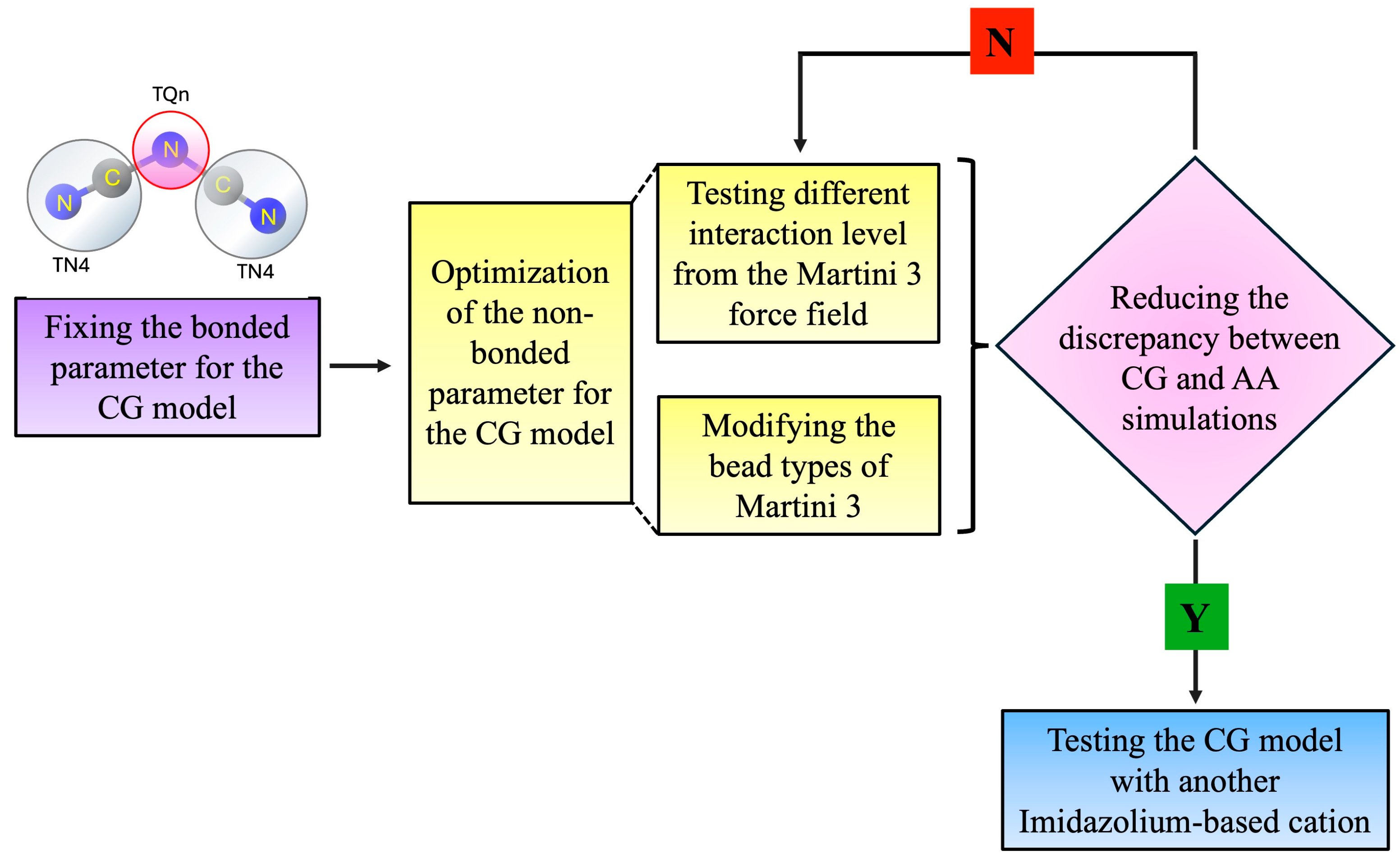
2.2. Coarse-Grained (CG) Model Parameterization

For CG molecular dynamics simulations, we employed the MARTINI 3 force field. For the [EMIM]+ cation, we adopted the model proposed by Vazquez-Salazar et al. [31] and developed our own MARTINI 3 CG model for the representation of the [DCA] anion. The CG [DCA] bead was represented by three beads, i.e., a central TQn bead (where n = 1–5) and two TN4 beads (shown in Figure 1B). The TN4 beads were adopted from the CG bead type of the -CN group (“TN4a”) proposed by Alessandri R. et al. [32]. A single TQ bead was selected to represent the central polar block, as it effectively models a single nitrogen atom within the structure. Our parameterization scheme for the [DCA] ion beads contained two parts. First, we developed bonded interaction parameters, and then we optimized the Lennard–Jones interaction (non-bonded) parameters between the beads on [DCA] ions.

2.2.1. Parameterization of Bonded Interactions

After the mapping of the molecule, we built the bonded parameter for the [DCA] anion from the AA trajectory (using OPLS-AMBER force field) of bulk IL. We considered MARTINI 3 to obtain the bead distance, as MARTINI 3 is based on the size and shape concept, with the center of geometry (COG)-based mapping [32], whereas MARTINI 2 is limited to the center of mass (COM) of the molecule and chemical group only. First, the AA trajectory is mapped into the CG format according to the COG-based strategy. From the mapped trajectory, we obtained the average bond and angle of the anion, which are further used as input parameters for the anion CG model.

2.2.2. Parameterization of Non-Bonded Interactions

Non-bonded interaction parameterization was performed in combination with modifying bead type and Lennard–Jones parameter. So, the CG model should be able to reproduce the important physicochemical and structural properties of IL (such as density and RDF). We calculated the radial distribution function (RDF) [g(r)] between the bead pairs because it gives us an idea about the local density of one bead with respect to other beads. For this analysis, we focused on two types of bead pair combinations: (a) cation–anion beads (intermolecular interaction) and (b) anion–anion beads (self-interaction). We excluded the cation–cation bead combinations from the calculation, as the CG model and parameters for the [EMIM]+ cation are already well-established and validated. [31]. Three bead pair combinations for anion–anion (self-interactions) and six bead pair combinations for cation–anion were obtained.

2.3. Coarse-Grained (CG) Simulation Setup

The equilibrated trajectory from the AA simulation was mapped into the CG model for further simulation. The CG simulation protocol is structured as follows. The energy-minimization step was initially completed using the steepest-descent algorithm to avoid clashes between the atoms. Thereafter, the equilibration steps were performed using both the NVT and NPT ensemble for a shorter time, followed by a production run using the NPT ensemble. Finally, for evaluation, we visually inspected the trajectory using VMD [33]. During the equilibration steps, the temperature was controlled using the velocity-rescaling (v-rescale) thermostat [34], while the Nosé–Hoover thermostat [27], with a coupling time of 1 ps, was employed for the production run. For pressure control, we utilized the Berendsen [35] pressure-coupling method at 1 bar during the equilibration phase. In the production run, we used the Parrinello–Rahman [28] barostat with compressibility of 3.0 × 10⁻⁵ bar−1 compressibility under isotropic conditions, maintaining the pressure at 1 bar. Long-range electrostatic forces were handled by a reaction field (RF) method [36]. We used the Potential Shift–Verlet coulomb modifier to calculate coulombic interaction energy beyond the cutoff value of 1.1 nm. The time step was 10.0 fs, and all the properties were computed from the trajectories stored at an interval of 25.0 ps during the production run.

3. Results and Discussion

3.1. Bonded-Interaction Parameterization

To obtain the accurate bond and angle with less discrepancy for the distribution between the AA and CG peaks, we adjusted the force-constant value (kb and kθ). We adopted the force constant (1,000,000 kJ/mol/nm2) for our TN4 beads, which is analogous to the previously used TN4a bead type reported by Alessandri R. et al. [32].
Subsequently, we fine-tuned the force constant value through manual adjustments to determine the optimal value for our system. Figure 1C,D show the probability distribution of the TQn-TN4 bond and TN4-TQn-TN4 angle for the AA and CG simulation using the final set of parameters. Table 1 lists the optimized bond and angle parameters of the anion that are further used for the CG simulation. Finally, the force constant obtained for bond and angle are 1,500,000 kJ/mol/nm2 and 700 kJ/mol/rad2, respectively, which are relatively higher than the previously mentioned values.

3.2. Non-Bonded Parameter for the [DCA] Anion BEADS

3.2.1. Testing All Types of Charged Beads (TQn) from the MARTINI 3 Force Field

We utilized IL’s molecular density (ρ) using AA and CG models. First, we tested all types of charged beads of the [DCA] anion TQn as n = 1 to 5 by fixing the TN4 bead, and then we compared the density, ρ (gm/cc) (T = 303.15 K), for both AA and CG models to minimize the error (Table 2). The density fluctuations from AA for both force fields, OPLS-AMBER and CHARMM, are within a similar range (shown in Supplementary Figure S2). After using the TQ5 bead, we found that the density of the IL did not fall within the 5–10% error range of the AA simulation data (Table 2). To develop a more accurate CG model that captures the AA density of the ionic liquid (IL), it is necessary to go beyond simply modifying the central TQn beads [31].
Furthermore, we analyzed the g(r) for the different bead pairs to evaluate the relative importance of non-bonded interactions in the system. As shown in Supplementary Figure S4, the g(r) for the pairs of anion beads (TQn-TQn, TN4-TN4, and TQn-TN4) between AA and CG simulations does not overlap well at 303.15 K, even after changing the anion bead type from TQ1 to TQ5. However, the g(r) between cation and anion bead pairs matches quite well for CG with AA, and even for the change in the anion bead type from TQ1 to TQ5 (as shown in Supplementary Figure S5). Indeed, the height and position of the first peak are close to each other, demonstrating that the used parameter of intermolecular interactions between cations and anions in our CG model is well-optimized and no further modification is needed. Therefore, in the herein study, we only focused on the parameterization of the non-bonded interactions among these anion beads.

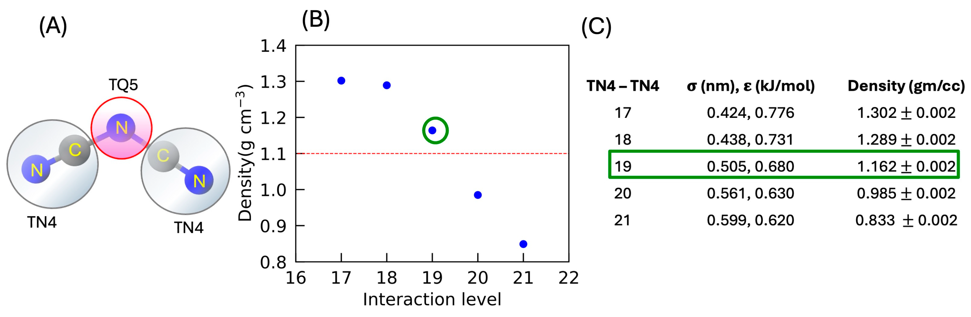
3.2.2. Changing the Interaction Level of the Anion Beads for MARTINI 3 Force Field

Both TQ1 and TQ5 beads effectively model the central nitrogen atom of the anion. However, the MARTINI 3 force-field interaction matrix profile showed that TQ5 interactions with SC6, TC6h, and TC5h cation beads are more accurate in reflecting the chemical nature of these components than TQ1. We started by fine-tuning the TN4-TN4 interactions by fixing all the other interaction parameters. Initially, the default interaction level for TN4 beads was set to 9, corresponding to σ = 0.340 nm and ε = 2.020 kJ/mol. This level falls within the intermediate interactions of beads, according to the recent MARTINI 3 release.
To further evaluate the model interaction level, we tested all the interaction levels, from intermediate (10) to super repulsive (21). By changing the self-interaction parameters, we obtained the molecular densities of the CG model (Supplementary Table S2). Figure 2B shows the molecular density (ρ) with respect to the self-interaction parameters for the TN4-TN4 beads at a temperature of 303.15 K. Meanwhile, Figure 2C represents the table of the self-interaction levels and their corresponding non-bonded parameters (σ and ε) with respect to the molecular density. In Figure 2B, the red horizontal line represents the density (ρ) obtained from the OPLS-AMBER (AA) force field. In Figure 2B, the ρ (gm/cc) obtained from the repulsive interaction at level 19 is marked with a green circle, showing a good alignment with the AA density (red horizontal line). The error between the density of our CG model and AA framework (OPLS-AMBER and CHARMM) is ~5.8% (Table 3), and according to the MARTINI CG framework, if the density deviation falls within 5–10% of AA values, the CG parameters are acceptable.

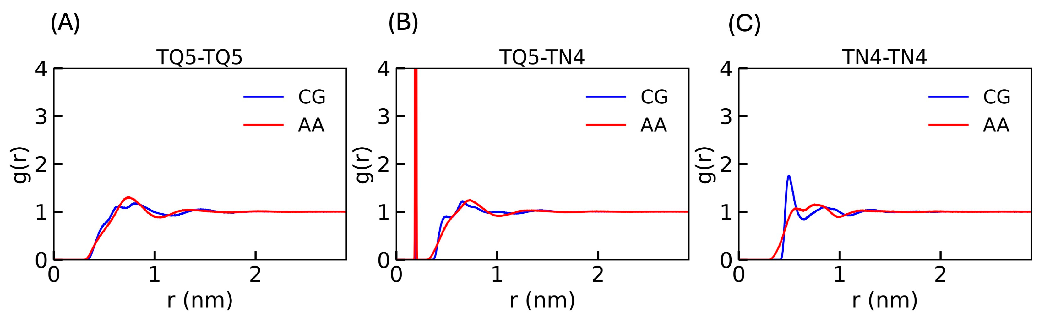
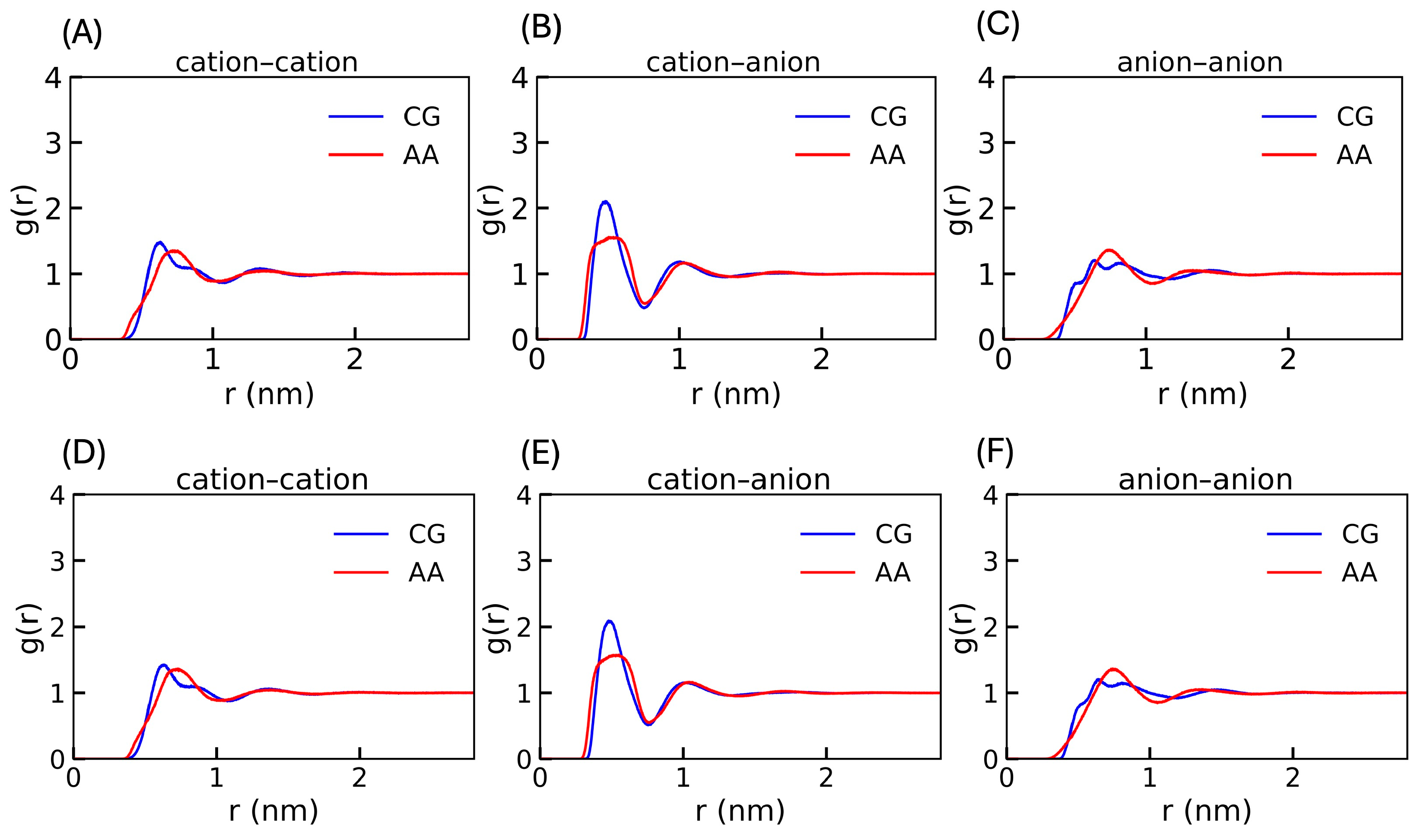
3.3. The Model Validation

We again checked the g(r) for the beads of the [DCA] anion with the interaction level 19 of TN4-TN4 beads. As mentioned before, a total of three combinations of bead pairs were considered for calculating g(r) for the beads of the [DCA] anion. The RDF (g(r)) values for the TQ5-TQ5, TQ5-TN4, and TN4-TN4 bead pairs are shown in Figure 3. These plots represent a comparison between the results from our CG model and the AA simulation data at a temperature of 303.15 K.
We found that g(r) for the charged bead anion pair TQ5-TQ5 for CG shows close agreement with the AA simulation data (shown in Figure 3A), as the position and height of the peak match well with each other. Figure 3B illustrates the distribution of TN4 beads of the anion relative to the TQ5 bead. These two beads are connected by a covalent bond (shown in Figure 2A). The first peak in the g(r) plot represents TQ5-TN4 bond.
The second peak in Figure 3B depicts the distribution of the intermolecular bead pair TQ5-TN4. Notably, this second peak shows a good alignment between the coarse-grained CG model and the AA data. Similarly, the g(r) of the TN4-TN4 beads is shown in Figure 3C. The distribution of the peak derived from the AA simulation exhibits a slight rightward shift compared to the peak obtained using the CG model. This slight deviation is expected due to the shift from AA to CG resolution. The simplification in the CG model results in the loss of some atomistic details where atoms are combined into larger CG beads, accounting for the minor differences in the distribution patterns. Supplementary Figure S6 illustrates the g(r) between the cation and anion bead pairs, showing the alignment in the position and height of the peaks between the CG and AA.
Now, it has become evident that our anion CG model and the self-interaction parameters have compatibility with the [EMIM]+ cation at 303.15 K. Now, it will be interesting to see whether our CG model will work at a higher 343.15 K temperature with the same [EMIM]+ cation. This helps us understand the temperature transferability of our designed CG model and further validation.
To address this question, we conducted a comparative analysis of the density and ion pair distributions in both AA and CG models at temperatures of 303.15 K and 343.15 K. At the higher temperature, 343.15 K, the density for the CG model is 1.118 gm/cc, which is close to the AA simulation data (Table 3). Figure 4 shows the g(r) for all ion pairs, the [[EMIM]+–[EMIM]+ cation, [EMIM]+ cation–[DCA] anion, and [DCA]–[DCA] anion. Here, r represents the distance between the center of mass (COM) of the ion pair. The RDF of the cation–cation of the CG model shows a good agreement with the AA model, as shown in Figure 4A,D. Similarly, in Figure 4B,E, the g(r) for cation–anion from the CG model is in close agreement with AA data. However, the g(r) peak in the AA resolution is broader and lower in height compared to the CG data. This discrepancy can be explained by the transitions from AA to CG resolution, which results in a 75% reduction in the system’s interaction sites, hence altering the interparticle distance. The RDF for the anion–anion pair also matches well for both AA and CG data, as shown in Figure 4C,F. These findings confirm the compatibility of our CG model and its self-interaction parameters with the [EMIM]+ cation at 303.15 K and 343.15 K.
We also checked the density to further validate its compactness at 343.15 K. The density of [EMIM][DCA] is 1.120 ± 0.003 (gm/cc), which agrees qualitatively with both experimental and AA data (OPLS-AMBER and CHARMM; Table 3).

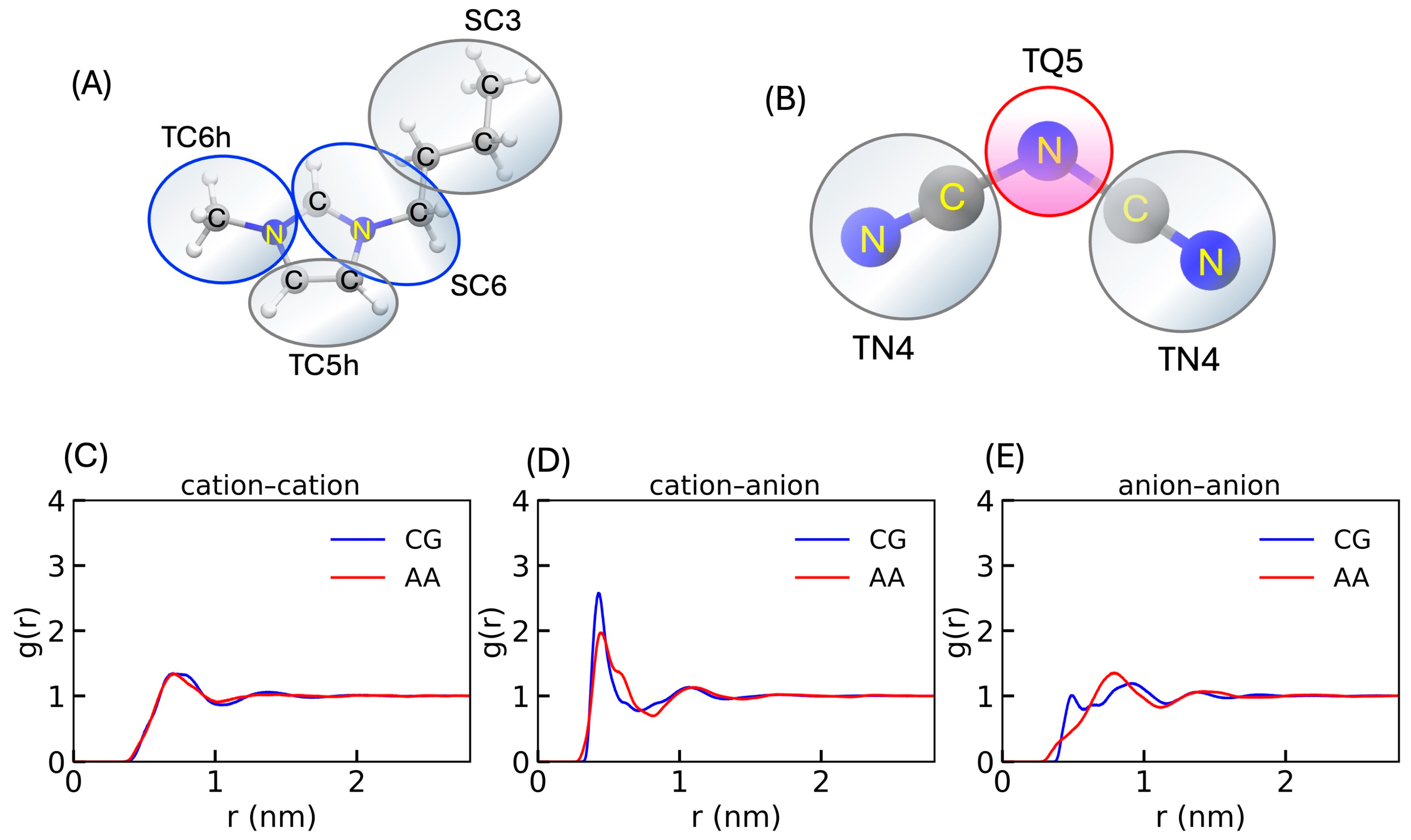
3.4. Validation of the CG Anion Model with Another Cation

Finally, we tested the model consistency in the presence of [BMIM]+ cation. We prepared the AA model of [BMIM] [DCA], and after the equilibration of trajectory, molecules were mapped into the CG model (shown in Figure 5). In this model, we used optimized non-bonded parameters (also mentioned in Figure 2) and bonded parameters from Table 1 for the [DCA] anion. Note, we considered [BMIM]+ parameters from Vazquez-Salazar et al. [31]. We calculated the average molecular density to validate the CG model. At 303.15 K, the density of [BMIM][DCA] is 1.099 ± 0.004 (gm/cc), which shows good agreement with the AA data of 1.075 ± 0.004 (gm/cc) and the experimental values reported in Ref. [38].
Next, we checked the g(r) for all the ion pairs: cation–cation, cation–anion, and anion–anion. As shown in Figure 5C–E, the g(r) for all the ion pairs from CG have aligned well with the AA data, confirming the accuracy of the CG anion model.

4. Conclusions

Here, we have presented a new CG-based model of a large organic anion such as dicyanamide [DCA] using the MARTINI 3 force field, employing a straightforward symmetrical approach for small-molecule parameterization. The workflow of the accurate CG model evaluation can be summarized as follows (Figure 6). First, we mapped the anion bead and fixed the bonded parameter based on the AA equilibrated trajectory. In the next step, we optimized the non-bonded parameter for anion. The optimization of the non-bonded parameters is a complicated procedure. Therefore, we tested both the interaction level and the modifying of the bead types of MARTINI 3, unless we obtained less discrepancy between CG and AA data. The matching of CG with AA data based on g(r) and molecular density (ρ) justifies our model accuracy, and furthermore, it can be used with another imidazolium-based cation.
As expected, our CG model shows compatibility with [BMIM]+. Furthermore, it reproduces the experimental molecular density (gm/cc) of ionic liquids (ILs) at the temperatures 303.15 and 343.15 K. The structural property, g(r), of the CG model shows good agreement with AA simulation data. The strategies for developing the CG model offer a straightforward approach for the accurate modeling of new small molecules. We will have the opportunity to use our CG model to study the micellization of non-ionic Pluronic in the [EMIM][DCA] IL medium.

Supplementary Materials

The following supporting information can be downloaded at https://www.mdpi.com/article/10.3390/physchem4040029/s1, Figure S1: Autocorrelation time of the density in different time intervals of (A) 10 ps, (B) 25 ps, (C) 50 ps, and (D) 100 ps, respectively; Figure S2: Density of the IL using different all-atom force fields. Density fluctuation of [EMIM][DCA] using CHARMM and OPLS-AMBER force field at 303.15 K temperature. Average values for density are shown inside the graph for CHARMM and OPLS-AMBER force fields; Figure S3: Representation of the [EMIM]+ cation, where atom names are labeled, also mentioned in Table S1; Figure S4: Radial distribution function [g(r)] of anion bead pairs with varying Qn (n = 1, 5) (charged bead). Top panel: g(r) for the pairs of anion beads (A) TQ1-TQ1, (B) TQ1-TN4 and (C)TN4-TN4 at 303.15 K temperature for CG and AA simulation. Bottom panel: the g(r) for the pairs of anion beads (D) TQ5-TQ5, (E) TQ5-TN4 and (F) TN4-TN4 at 303.15 K temperature for CG and AA simulation; Figure S5: Radial distribution function [g(r)] of cation-anion bead pairs with varying Qn (n = 1, 5) (charged bead). Top panel: g(r) between the bead pairs (A) TQ1-SC6, (B) TQ1-TC6h, (C) TQ1- TC5h, (D) TN4-SC6, (E) TN4-TC6h, and (F) TN4-TC5h at 303.15 K temperature for CG and AA simulation. Bottom panel: g(r) between the bead pairs (G) TQ5-SC6, (H)TQ5-TC6h, (I) TQ5-TC5h, (J) TN4-SC6, (K) TN4-TC6h and (L) TN4-TC5h for CG and AA simulation at 303.15 K temperature; Figure S6: Radial distribution function [g(r)] of cation-anion bead pairs using the optimized self-interaction parameter (non-bonded) for TN4 beads. The plot shows the radial distribution function [g (r)] between the six pairs of beads (A) TQ5-SC6, (B) TQ5-TC6h, (C) TQ5-TC5h, (D) TN4-SC6, (E)TN4-TC6h and (F) TN4-TC5h for CG and AA simulation at 303.15 K temperature; Table S1: Charge Distribution of the [EMIM]+ Cation based on CHARMM Framework (Note: atom names correspond to the labeling in Figure S3); Table S2: Comparison of the average density of [EMIM][DCA] bulk system using different interaction levels and their corresponding σ and ε to represent the self-interaction of TN4 beads.

Author Contributions

Conceptualization, S.K. and S.C.; methodology, S.K.; software, S.K.; validation, S.K.; investigation, S.K. and S.C.; resources, S.C.; data curation, S.K.; writing—original draft preparation, S.K.; writing—review and editing, S.K. and A.E.; visualization, S.K. and S.C.; supervision, S.C.; project administration, S.C.; funding acquisition, S.C. All authors have read and agreed to the published version of the manuscript.

Funding

This research was funded by DMREF (grant number 2323317) for this work.

Data Availability Statement

Data are contained within the article and Supplementary Materials.

Acknowledgments

Author acknowledges the HPC resources from the Advanced Cyberinfrastructure for Education and Research (ACER) at the University of Illinois Chicago (UIC) for providing computing facilities. We thank Xiaoli Yan for his technical assistance.

Conflicts of Interest

The authors declare no conflicts of interest.

References

  1. Chiappe, C.; Pieraccini, D. Ionic Liquids: Solvent Properties and Organic Reactivity. J. Phys. Org. Chem. 2005, 18, 275–297. [Google Scholar] [CrossRef]
  2. Ueno, K.; Tokuda, H.; Watanabe, M. Ionicity in Ionic Liquids: Correlation with Ionic Structure and Physicochemical Properties. Phys. Chem. Chem. Phys. 2010, 12, 1649. [Google Scholar] [CrossRef] [PubMed]
  3. Chang, J.-C.; Ho, W.-Y.; Sun, I.-W.; Chou, Y.-K.; Hsieh, H.-H.; Wu, T.-Y. Synthesis and Properties of New Tetrachlorocobaltate (II) and Tetrachloromanganate (II) Anion Salts with Dicationic Counterions. Polyhedron 2011, 30, 497–507. [Google Scholar] [CrossRef]
  4. Vafaeezadeh, M.; Alinezhad, H. Brønsted Acidic Ionic Liquids: Green Catalysts for Essential Organic Reactions. J. Mol. Liq. 2016, 218, 95–105. [Google Scholar] [CrossRef]
  5. Fumino, K.; Peppel, T.; Geppert-Rybczyńska, M.; Zaitsau, D.H.; Lehmann, J.K.; Verevkin, S.P.; Köckerling, M.; Ludwig, R. The Influence of Hydrogen Bonding on the Physical Properties of Ionic Liquids. Phys. Chem. Chem. Phys. 2011, 13, 14064. [Google Scholar] [CrossRef]
  6. Pottkämper, J.; Barthen, P.; Ilmberger, N.; Schwaneberg, U.; Schenk, A.; Schulte, M.; Ignatiev, N.; Streit, W.R. Applying Metagenomics for the Identification of Bacterial Cellulases That Are Stable in Ionic Liquids. Green Chem. 2009, 11, 957–965. [Google Scholar] [CrossRef]
  7. Pinkert, A.; Marsh, K.N.; Pang, S.; Staiger, M.P. Ionic Liquids and Their Interaction with Cellulose. Chem. Rev. 2009, 109, 6712–6728. [Google Scholar] [CrossRef]
  8. Köddermann, T.; Paschek, D.; Ludwig, R. Molecular Dynamic Simulations of Ionic Liquids: A Reliable Description of Structure, Thermodynamics and Dynamics. ChemPhysChem 2007, 8, 2464–2470. [Google Scholar] [CrossRef]
  9. Elaiwi, A.; Hitchcock, P.B.; Seddon, K.R.; Srinivasan, N.; Tan, Y.M.; Welton, T.; Zora, J.A. Hydrogen Bonding in Imidazolium Salts and Its Implications for Ambient-Temperature Halogenoaluminate(III) Ionic Liquids. J. Chem. Soc. Dalton Trans. 1995, 21, 3467–3472. [Google Scholar] [CrossRef]
  10. Freemantle, M. Designer Solvents. Chem. Eng. News Arch. 1998, 76, 32–37. [Google Scholar] [CrossRef]
  11. Sun, Z.; Zheng, L.; Zhang, Z.Y.; Cong, Y.; Wang, M.; Wang, X.; Yang, J.; Liu, Z.; Huai, Z. Molecular Modelling of Ionic Liquids: Situations When Charge Scaling Seems Insufficient. Molecules 2023, 28, 800. [Google Scholar] [CrossRef] [PubMed]
  12. Crespo, E.A.; Schaeffer, N.; Coutinho, J.A.P.; Perez-Sanchez, G. Improved Coarse-Grain Model to Unravel the Phase Behavior of 1-Alkyl-3-Methylimidazolium-Based Ionic Liquids through Molecular Dynamics Simulations. J. Colloid Interface Sci. 2020, 574, 324–336. [Google Scholar] [CrossRef] [PubMed]
  13. Pérez-Sánchez, G.; Schaeffer, N.; Lopes, A.M.; Pereira, J.F.B.; Coutinho, J.A.P. Using Coarse-Grained Molecular Dynamics to Understand the Effect of Ionic Liquids on the Aggregation of Pluronic Copolymer Solutions. Phys. Chem. Chem. Phys. 2021, 23, 5824–5833. [Google Scholar] [CrossRef]
  14. Pérez-Sánchez, G.; Vicente, F.A.; Schaeffer, N.; Cardoso, I.S.; Ventura, S.P.M.; Jorge, M.; Coutinho, J.A.P. Unravelling the Interactions between Surface-Active Ionic Liquids and Triblock Copolymers for the Design of Thermal Responsive Systems. J. Phys. Chem. B 2020, 124, 7046–7058. [Google Scholar] [CrossRef]
  15. Karimi-Varzaneh, H.A.; Müller-Plathe, F.; Balasubramanian, S.; Carbone, P. Studying Long-Time Dynamics of Imidazolium-Based Ionic Liquids with a Systematically Coarse-Grained Model. Phys. Chem. Chem. Phys. 2010, 12, 4714–4724. [Google Scholar] [CrossRef]
  16. Bhargava, B.L.; Devane, R.; Klein, M.L.; Balasubramanian, S. Nanoscale Organization in Room Temperature Ionic Liquids: A Coarse Grained Molecular Dynamics Simulation Study. Soft Matter 2007, 3, 1395–1400. [Google Scholar] [CrossRef]
  17. Kodirov, A.; Abduvokhidov, D.; Mamatkulov, S.; Shahzad, A.; Razzokov, J. The Absorption Mechanisms of CO2, H2S and CH4 Molecules in [EMIM][SCN] and [EMIM][DCA] Ionic Liquids: A Computational Insight. Fluid Phase Equilibria 2024, 581, 114080. [Google Scholar] [CrossRef]
  18. Abraham, M.J.; Murtola, T.; Schulz, R.; Páll, S.; Smith, J.C.; Hess, B.; Lindah, E. Gromacs: High Performance Molecular Simulations through Multi-Level Parallelism from Laptops to Supercomputers. SoftwareX 2015, 1, 19–25. [Google Scholar] [CrossRef]
  19. Hockney, R.W.; Goel, S.P.; Eastwood, J.W. Quiet High-Resolution Computer Models of a Plasma. J. Comput. Phys. 1974, 14, 148–158. [Google Scholar] [CrossRef]
  20. Mayne, C.G.; Saam, J.; Schulten, K.; Tajkhorshid, E.; Gumbart, J.C. Rapid Parameterization of Small Molecules Using the Force Field Toolkit. J. Comput. Chem. 2013, 34, 2757–2770. [Google Scholar] [CrossRef]
  21. Cadena, C.; Anthony, J.L.; Shah, J.K.; Morrow, T.I.; Brennecke, J.F.; Maginn, E.J. Why Is CO2 so Soluble in Imidazolium-Based Ionic Liquids? J. Am. Chem. Soc. 2004, 126, 5300–5308. [Google Scholar] [CrossRef] [PubMed]
  22. Cadena, C.; Maginn, E.J. Molecular Simulation Study of Some Thermophysical and Transport Properties of Triazolium-Based Ionic Liquids. J. Phys. Chem. B 2006, 110, 18026–18039. [Google Scholar] [CrossRef] [PubMed]
  23. Frisch, M.J.; Trucks, G.W.; Schlegel, H.B.; Scuseria, G.E.; Robb, M.A.; Cheeseman, J.R.; Scalmani, G.; Barone, V.; Mennucci, B.; Petersson, G.A.; et al. Gaussian, Version 16, Revision B.01; Gaussian Inc.: Wallingford, CT, USA, 2016. [Google Scholar]
  24. Canongia Lopes, J.N.; Pádua, A.A.H. Molecular Force Field for Ionic Liquids III: Imidazolium, Pyridinium, and Phosphonium Cations; Chloride, Bromide, and Dicyanamide Anions. J. Phys. Chem. B 2006, 110, 19586–19592. [Google Scholar] [CrossRef] [PubMed]
  25. Lopes, J.N.C.; Deschamps, J.; Pádua, A.A.H. Modeling Ionic Liquids Using a Systematic All-Atom Force Field. J. Phys. Chem. B 2004, 108, 2038–2047. [Google Scholar] [CrossRef]
  26. Martínez, L.; Andrade, R.; Birgin, E.G.; Martínez, J.M. PACKMOL: A Package for Building Initial Configurations for Molecular Dynamics Simulations. J. Comput. Chem. 2009, 30, 2157–2164. [Google Scholar] [CrossRef]
  27. Nosé, S. A Unified Formulation of the Constant Temperature Molecular Dynamics Methods. J. Chem. Phys. 1984, 81, 511–519. [Google Scholar] [CrossRef]
  28. Parrinello, M.; Rahman, A. Polymorphic Transitions in Single Crystals: A New Molecular Dynamics Method. J. Appl. Phys. 1981, 52, 7182–7190. [Google Scholar] [CrossRef]
  29. Darden, T.; York, D.; Pedersen, L. Particle Mesh Ewald: An N Log(N) Method for Ewald Sums in Large Systems. J. Comput. Chem. 1993, 98, 10089–10092. [Google Scholar] [CrossRef]
  30. Hess, B.; Bekker, H.; Berendsen, H.J.C.; Fraaije, J.G.E.M. LINCS: A Linear Constraint Solver for Molecular Simulations. J. Comput. Chem. 1997, 18, 1463–1472. [Google Scholar] [CrossRef]
  31. Vazquez-Salazar, L.I.; Selle, M.; De Vries, A.H.; Marrink, S.J.; Souza, P.C.T. Martini Coarse-Grained Models of Imidazolium-Based Ionic Liquids: From Nanostructural Organization to Liquid-Liquid Extraction. Green Chem. 2020, 22, 7376–7378. [Google Scholar] [CrossRef]
  32. Alessandri, R.; Barnoud, J.; Gertsen, A.S.; Patmanidis, I.; de Vries, A.H.; Souza, P.C.T.; Marrink, S.J. Martini 3 Coarse-Grained Force Field: Small Molecules. Adv. Theory Simul. 2022, 5, 2100391. [Google Scholar] [CrossRef]
  33. Humphrey, W.; Dalke, A.; Schulten, K. VMD: Visual Molecular Dynamics. J. Mol. Graph. 1996, 1, 33–38. [Google Scholar] [CrossRef] [PubMed]
  34. Bussi, G.; Donadio, D.; Parrinello, M. Canonical Sampling through Velocity Rescaling. J. Chem. Phys. 2007, 126, 14101. [Google Scholar] [CrossRef] [PubMed]
  35. Berendsen, H.J.C.; Postma, J.P.M.; Van Gunsteren, W.F.; Dinola, A.; Haak, J.R. Molecular Dynamics with Coupling to an External Bath. J. Chem. Phys. 1984, 81, 3684–3690. [Google Scholar] [CrossRef]
  36. Tironi, I.G.; Sperb, R.; Smith, P.E.; Van Gunsteren, W.F. A Generalized Reaction Field Method for Molecular Dynamics Simulations. J. Chem. Phys. 1995, 102, 5451–5459. [Google Scholar] [CrossRef]
  37. Quijada-Maldonado, E.; Van Der Boogaart, S.; Lijbers, J.H.; Meindersma, G.W.; De Haan, A.B. Experimental Densities, Dynamic Viscosities and Surface Tensions of the Ionic Liquids Series 1-Ethyl-3-Methylimidazolium Acetate and Dicyanamide and Their Binary and Ternary Mixtures with Water and Ethanol at T = (298.15 to 343.15 K). J. Chem. Thermodyn. 2012, 51, 51–58. [Google Scholar] [CrossRef]
  38. Larriba, M.; Navarro, P.; Julián García, J.; Rodríguez, F. Liquid−Liquid Extraction of Toluene from Heptane Using [Emim][DCA], [Bmim][DCA], and [Emim][TCM] Ionic Liquids. Ind. Eng. Chem. Res. 2013, 52, 2341–2720. [Google Scholar] [CrossRef]
Figure 1. CG representation of [EMIM][DCA] and bonded parameter for [DCA] anion. The mapping approach used to model the (A) [EMIM]+ cation (note: bond distance for [EMIM]+ cation beads kept constraint with a value of 0.315, 0.285, and 0.285 nm for TC6h-TC5h, SC6-TC6h, and SC6-TC5h, respectively) and (B) [DCA] anion beads. Here, the blue-colored shape represents the positively charged beads for TC6h and SC6, whereas the red represents the negatively charged bead for TQn. The grey color represents apolar beads for TC5h, TN4. Probability distribution of (C) TQn-TN4 bond distance and (D) TN4-TQn-TN4 angle from AA and CG simulation.
Physchem 04 00029 g001
Figure 2. Optimization of the non-bonded parameters for the beads of [DCA] anion by utilizing the molecular density [ρ(gm/cc)] measurement. (A) schematic representation of the beads for [DCA] anion. (B) Density value of bulk IL at 303.15 K temperature by tuning the self-interaction for the TN4 beads. (C) Interaction level and their corresponding σ and ε for the TN4 beads and obtained density values.
Physchem 04 00029 g002
Figure 3. Evaluation of the structural properties for [DCA] anion using the optimized self-interaction level 19 of TN4 beads. (AC) Radial distribution function (g(r)) for the three bead pairs TQ5-TQ5, TQ5-TN4, and TN4-TN4, respectively, at a temperature of 303.15 K.
Physchem 04 00029 g003
Figure 4. Radial distribution function [g(r)] of ion pairs at different temperatures using the optimized non-bonded parameters. (AC) Display of the g(r) between the center of mass (COM) of cation–cation, cation–anion, and anion–anion pairs, respectively, for both AA and CG models at 303.15 K. (DF) Display of the g(r) between the center of mass (COM) of cation–cation, cation–anion, and anion–anion pairs, respectively, for both AA and CG models at 343.15 K.
Physchem 04 00029 g004
Figure 5. Validation of CG anion model to a different ionic liquid with [BMIM]+ cation. CG model of (A) anion [DCA] and (B) cation [BMIM]+. (CE) Display of the g(r) between the center of mass (COM) of cation–cation, cation–anion, and anion–anion pairs, respectively, for both AA and CG models at 303.15 K.
Physchem 04 00029 g005
Figure 6. Workflow for the evaluation of CG model for the [DCA] anion. The development of the [DCA] anion’s CG model involves the tuning of both bonded and non-bonded parameters through the outlined steps. Bonded parameters are derived from AA simulation, while non-bonded parameters are tuned by systematically testing and adjusting bead types and interaction levels within the MARTINI 3 force-field framework.
Physchem 04 00029 g006
Table 1. Bonded parameter for the bead types in [DCA] anion in CG framework.
Beads TypeBond (nm)Kb (kj/mol/nm2)
TQn-TN40.19281,500,000
Beads TypeAngle (°)Kθ (kj/mol/rad2)
TN4-TQn-TN4128.05700
Table 2. Density comparison of [EMIM][DCA] IL bulk system at 303.15 K: AA versus CG simulations with varying central bead types for the [DCA] anion.
Beads Type (CG)Density (gm/cc)
TQ11.422 ± 0.003
TQ21.417 ± 0.003
TQ31.400 ± 0.003
TQ41.379 ± 0.003
TQ51.356 ± 0.004
All-atom (AA) simulations
OPLS-AMBER1.104 ± 0.003
CHARMM1.100 ± 0.003
Table 3. Comparison of the average density of [EMIM][DCA] bulk system using three methods: coarse-grained (CG) simulations, all-atomistic simulations (employing both CHARMM and OPLS-AMBER force fields), and experimental techniques. Measurements were taken at two temperatures: 303.15 K and 343.15 K. The percentage (%) deviation of density values was calculated using the AA (OPLS-AMBER) values as the reference.
ρ (gm/cc)Experiment [37]OPLS-AMBERCHARMMCoarse-Grain (CG)
T = 303.15 K1.098661.104 ± 0.003 (+0.5%)1.100 ± 0.003 (+0.4%)1.162 ± 0.004 (+5.8%)
T = 343.15 K1.072771.077 ± 0.003 (+0.4%)1.072 ± 0.003 (−0.3%)1.118 ± 0.002 (+4.1%)
Disclaimer/Publisher’s Note: The statements, opinions and data contained in all publications are solely those of the individual author(s) and contributor(s) and not of MDPI and/or the editor(s). MDPI and/or the editor(s) disclaim responsibility for any injury to people or property resulting from any ideas, methods, instructions or products referred to in the content.

