1. Introduction
Asphalt binder grades are critical to pavement design. The current classification system, Superpave performance grading (PG), differentiates binders according to their susceptibility to failures that occur at high and low temperatures. The first number in a grade indicates the high-temperature performance. The higher this temperature, the stiffer the binder and the less susceptible the binder is to permanent deformation at high temperatures. The second, negative number, indicates the low-temperature performance. The lower this temperature, the less susceptible the binder is to thermal cracking at low temperatures. At higher temperatures, the preferred performance is a stiffer binder to resist permanent deformation. At lower temperatures, the preferred performance is a softer binder to resist thermal cracking. The PG system guides pavement design according to the temperature range that the road will experience. The larger the range between the two numbers, the better performing the binder.
To determine the PG of a binder for pavement design, at least two days of testing are needed. The binder undergoes different aging simulations that require hours of time and energy. The high PG is determined by the initial and the short-term aged viscoelastic properties. Short-term aging requires the heating and rotating of a sample of binder for 85 min at 163 °C. This aging process mimics the mixing and compaction process. The viscoelastic testing requires about an hour depending on how many temperatures are evaluated. The low PG evaluates the binder that is prepared with the pressure aging vessel (PAV). The PAV keeps the sample at 100 °C (moderate climates) and 2.07 MPA for 20 h. Using chemical methods to indicate physical properties could save time, energy, and money.
NMR relaxometry has been developed over the years to fit industry applications. From paint aging to SBS determination in asphalt pavement, polymer systems have been shown to have distinct NMR relaxation times that can be related to physical properties [
1,
2,
3,
4,
5,
6,
7,
8,
9,
10]. While investigating asphalt is a relatively new application, most studies have relied on
T2 relaxation methods.
T2 methods have indicated characteristic NMR relaxation times for components of asphalt binder [
11,
12].
T2 analysis has also been used to describe asphaltene aggregation [
13] and indicate penetration grades [
14]. While
T2 is a faster method, it relies on solvents that destroy the structural integrity of the sample [
15]. Additionally, since
T2 acquisition is so fast, solid-state relaxation can be hard to detect at higher field strength. Therefore, to probe into the asphalt structural integrity, this work focuses on the lesser-used
T1 relaxation.
Recently,
T1 NMR relaxometry has been shown to indicate viscoelastic changes in asphalt binder due to additives [
16] and aging [
17]. Generally, a longer relaxation time describes a stiffer binder. Additionally, rejuvenation mechanisms [
18] and mixture properties [
19] have been detected.
T1 relaxometry is a superior method since solvents and heat are not needed, preserving the molecular integrity. The major drawback of
T1 NMR relaxometry testing is the time and knowledge needed to analyze the results. One dataset acquisition can require up to 10 h, and analysis can take several extra hours. Previous NMR work conducted on asphalt field testing resulted in a testing time of 20 min per location [
20]. Compared to physical testing which requires days, NMR is a superior acquisition method.
In this study, different grades and sources of asphalt binder are compared with NMR relaxometry. The complexity and time of this analysis was varied to determine the best and fastest fit of NMR
T1 relaxation data using sum-of-squares analysis (X
2). This analysis is used to separate chemical information from physical noise [
21]. Further, a least squares analysis was used to determine the relaxation constants. This analysis aims to compare PG asphalt binders quickly and effectively using NMR
T1 relaxation times from noisy experimental data.
2. Materials and Methods
Performance grade (PG) 64-22, 76-22, and 94-10 binders were sourced from Philips 66 in Granite City, IL, USA. Two separate batches of PG 64-22 were considered: PG 64-22 and 64-22 B. PG 64-22 binders are commonly found in the Midwest, while the stiffer qualities of the PG 76-22 could be utilized in warmer climates. The PG 94-10 would be too stiff to use practically but represents very aged binders.
In our study, 2 mm capillary tubes were dipped in the heated binders to ensure a uniform testing area, using the chocolate-covered pretzel method [
16,
17,
18,
19]. The 2 mm capillaries were then placed in 5 mm NMR sample tubes. A Bruker Avance DRX 200-MHz spectrometer was used to collect the
1H NMR
T1 relaxation data. The SIP-R pulse sequence was used to obtain exponential decays to zero instead of the traditional rise to maximum [
22]. The recovery delays were equidistant on a log scale to determine the shape of the exponential decay. Four scans, 5 s pre-delay, and 100 µs dead time were also used for data acquisition. The delay-dependent signals were fitted to 128 predefined coefficients logarithmically spaced from 0.1 ms to 1 s using an inverse Laplace transform (ILT). These parameters, relaxation times, and intensities are traditionally solved with an iterative inverse Laplace transform [
11,
23,
24]. The ILT results in an equation, as seen in Equation (1), but many of the 128 coefficients are zero. In Equation (1),
S(
τ) is the signal intensity for a given delay time τ;
T1 values indicate the relaxation times.
Since this analysis of 128 coefficients can take hours, simple multiexponential fits were also used to fit 1, 2, and 3 relaxation times to compare them to the best fit ILT. These multiexponential fits were developed using the curve fit function provided by the SciPy python library to model the relaxation data. The maximum number of solvable parameters depends on the number of data points acquired. Mono, bi, and tri exponential fits are simpler and faster ways to approximate complex exponential decays. Most relaxation data of asphalt binders contain one reliable primary relaxation time. These relaxation times are related to physical properties of a material [
16,
17]. After the primary
T1 relaxation time is determined, the relative ratio (
R1) can also be calculated by Equation (2).
S1 and
S2 are the signal intensities of the primary and secondary relaxation times,
T1,1 and
T1,2, respectively.
The number of data points was also reduced from 256, 64, 16, and 8. The reduced datasets were selected from the original 256, spaced equidistant on a log scale. Unlike the ILT analysis, which requires no a priori information, initial conditions and parameter bounds had to be specified. The initial intensity condition was set to the first, highest intensity. The initial conditions were set to 0.5, 0.005, and 0.0005 for the first, second, and third
T1 times. These values were chosen by visually examining the exponential decays for approximate relaxation times. The goodness of fit was investigated for 256, 64, 16, and 8 data points. One, two, and three exponentials were considered using the minimum least squares method, as shown in Equation (3).
Oi is the observed value, E
i the expected value, and X
2 the sum of error squared. The expected value was derived from fitting the
T1 and intensity constants in the multiexponential decay. Observed data are considered experimental data.
The objective of this study was to determine the optimal number of terms that would best fit the experimental data, specifically assessing how many exponentials were needed for an accurate fit. All parameters were bound to be greater than zero since intensities and time constants cannot have negative values. The average primary relaxation time and standard deviation (error bars) of three samples were compared in all experiments.
3. Results
All binders had a primary inflection point/relaxation time around 0.4–0.6 s, but this value shifts slightly. This shifting depended on the influence of noise from the device, the fit used, the number of points acquired, and the type of binder. The testing that would require the most time was the 256 data points transformed through the ILT. Eight data points transformed with a monoexponential fit would require the least amount of time and analysis. The objective of this analysis was a balance between time and fitting quality.
3.1. Noise
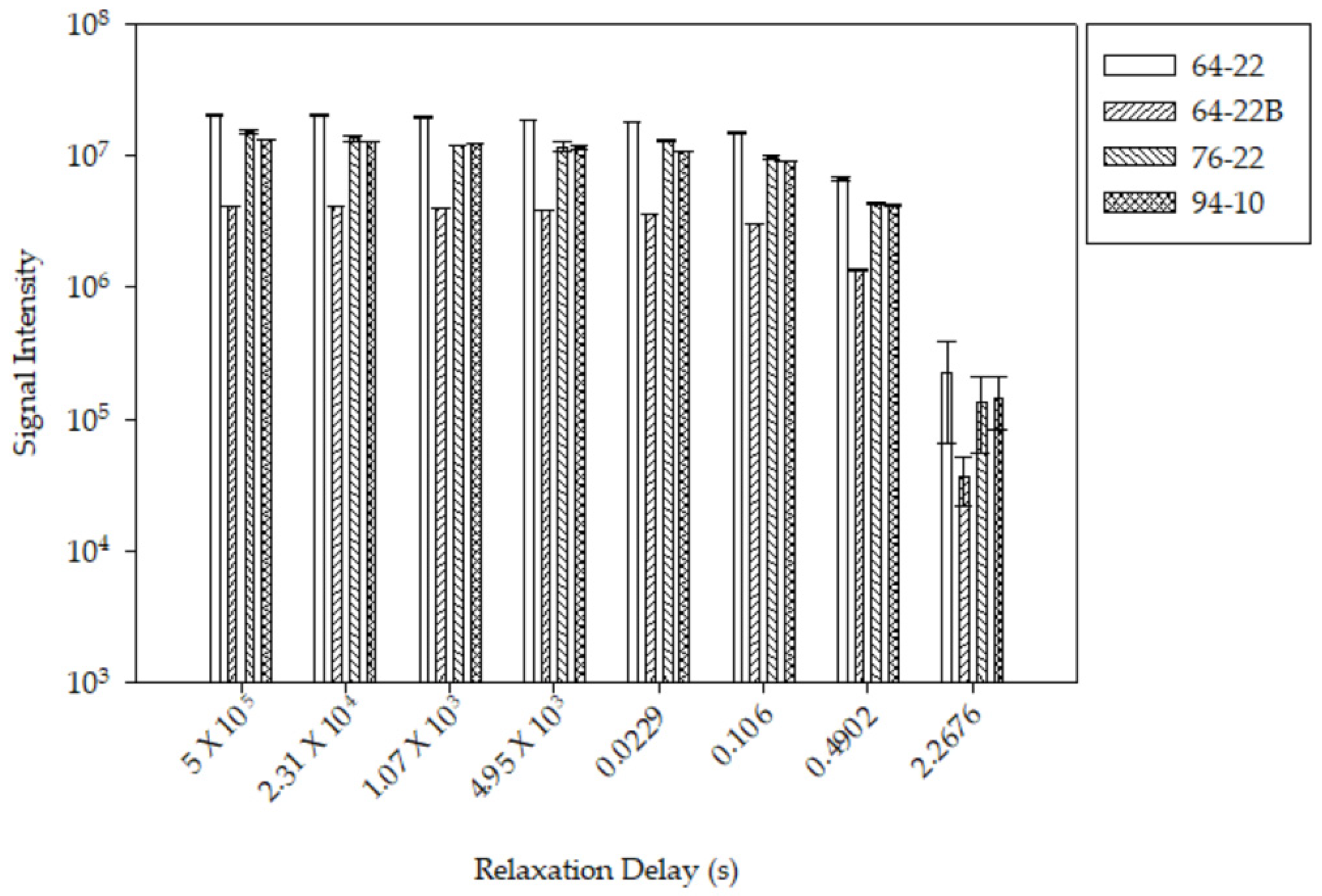
The noise from the device was not as impactful in the shifting of
T1 times, considering the scale of the intensities, as seen in
Figure 1. The average intensity of 32 scans of the same eight points was used to compare the standard deviation (error bars) of each sample. The most noise was seen at the 2.27 s relaxation delay. This occurred since the main signal had completely decayed at that point and the only thing remaining was noise.
3.2. Goodness of Fit
Goodness of fit is defined as the square of the difference between the expected value and the observed value. This criterion was used to determine the best-fitting algorithm between 1, 2, and 3 exponentials, as shown in
Figure 2. Unlike other statistical tests like ANOVA and
t-test, where a hypothesis is being tested, the least squares criterion provides the maximum likelihood estimator for quality of fit [
21]. Reference graphs can be found in
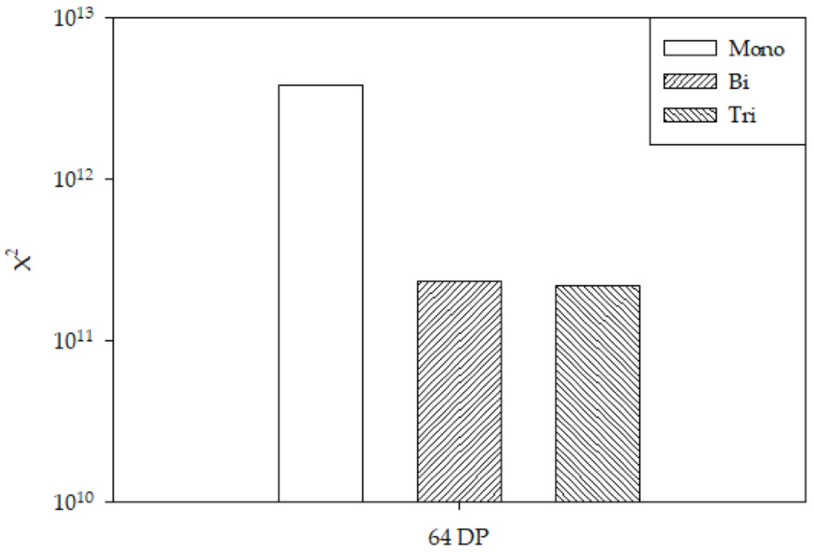
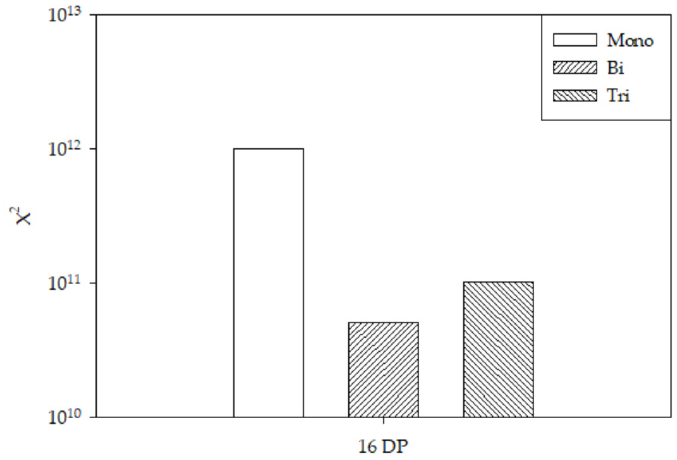
Appendix A. For all PG binders, the monoexponential fit was the worst. The biexponential and triexponential fit produced comparable results. In general, the triexponential was slightly better but did not provide much confidence when eight data points were used. Additionally, the triexponential fit overfit the 64-22 binders, skewing the primary ratio. Therefore, the best comparative fit for the binders was a biexponential fit. These values were acquired by fitting the curve against the objective function then squaring the difference between the predicted curve and the dataset. This pattern repeats for 256, 64, 16, and 8 data points.
3.3. Number of Data Points
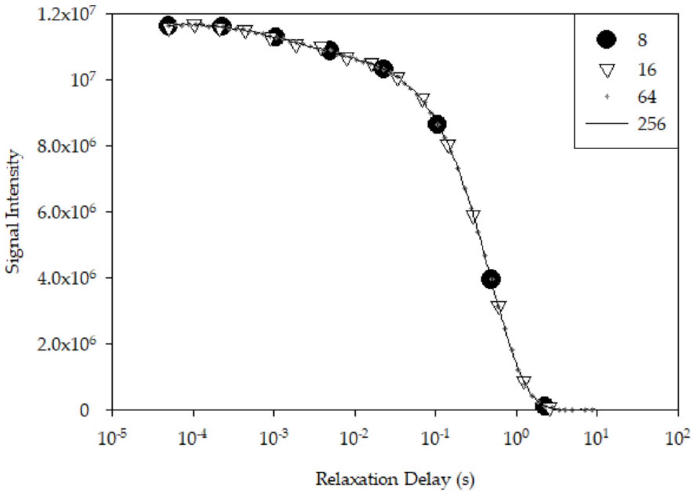
A total of 256 data points were acquired from an exponential decay for each binder sample. Out of those points, 64, 16, and 8 equally log-spaced points were sampled, as displayed in
Figure 3. Reducing the number of data points reduced the required testing time, as summarized in
Table 1. However, as the number of data points decreased, so did the ability to catch certain relaxation times, which appear as inflection points on the log scale. When reduced to eight data points, the standard deviation of some of the samples greatly increased. Sixty-four and sixteen points are viable reductions to consider as they reduce testing time and still allow for some differentiation. Eight points can be used to differentiate the PG 64-22 from the 76-22, but due to additional relaxation times, the 94-10 required more points to fit the relaxation times accurately.
3.4. Best and Fastest T1 Fits
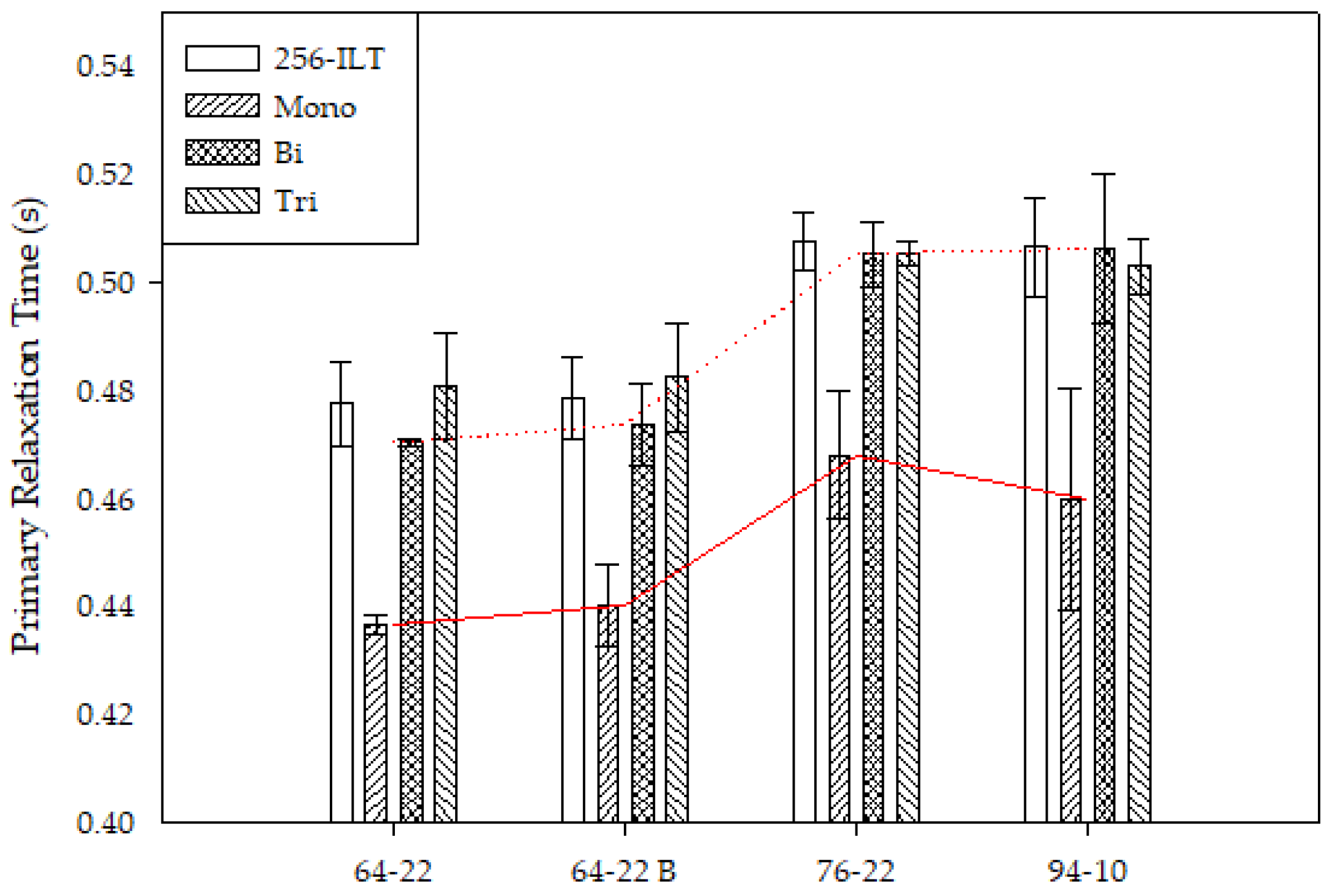
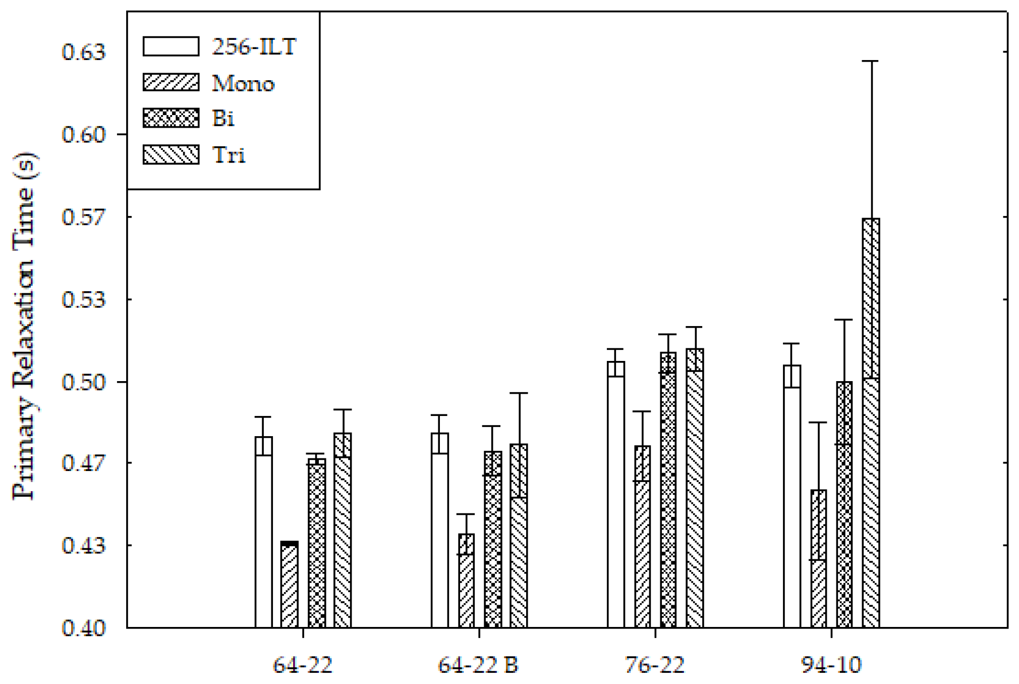
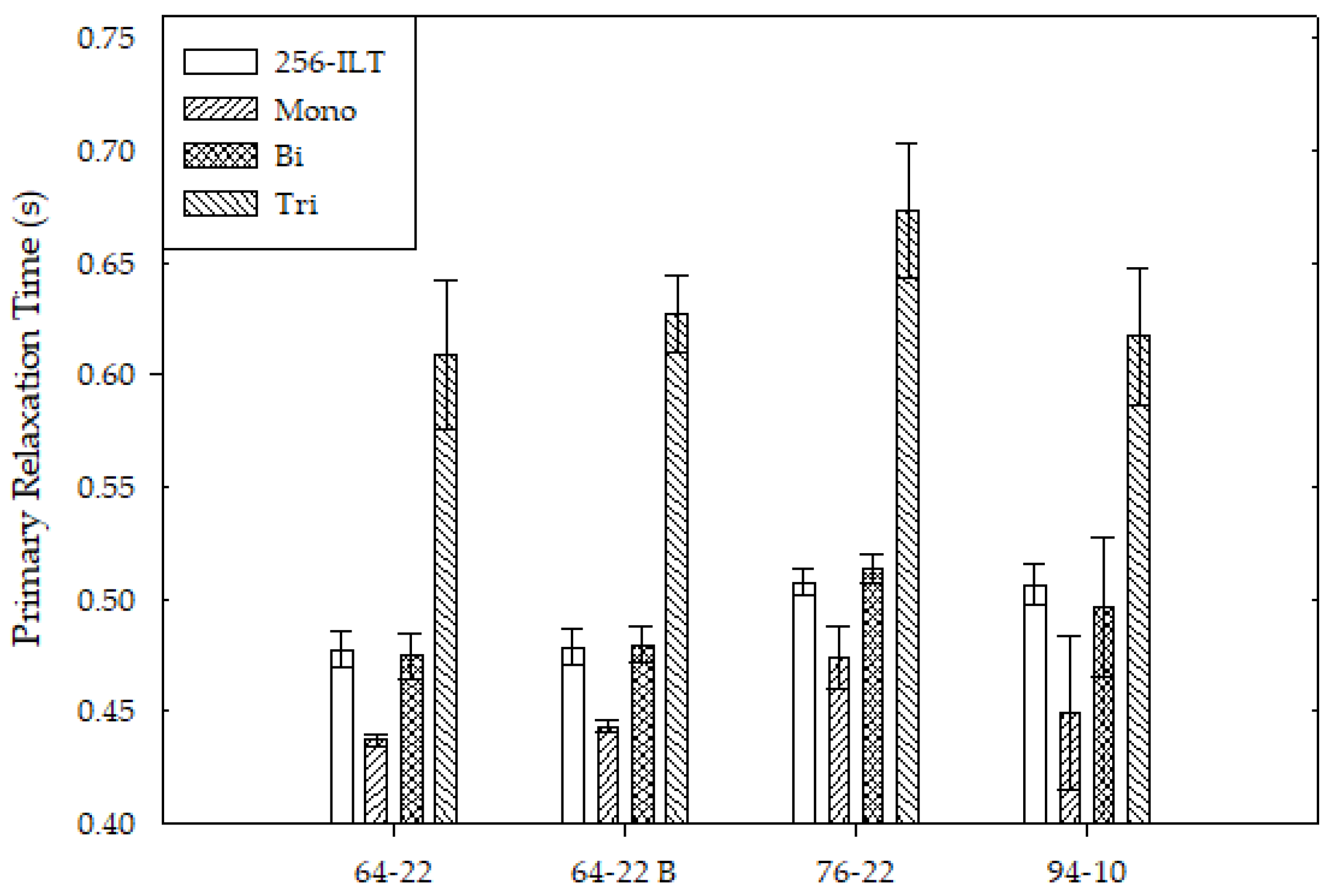
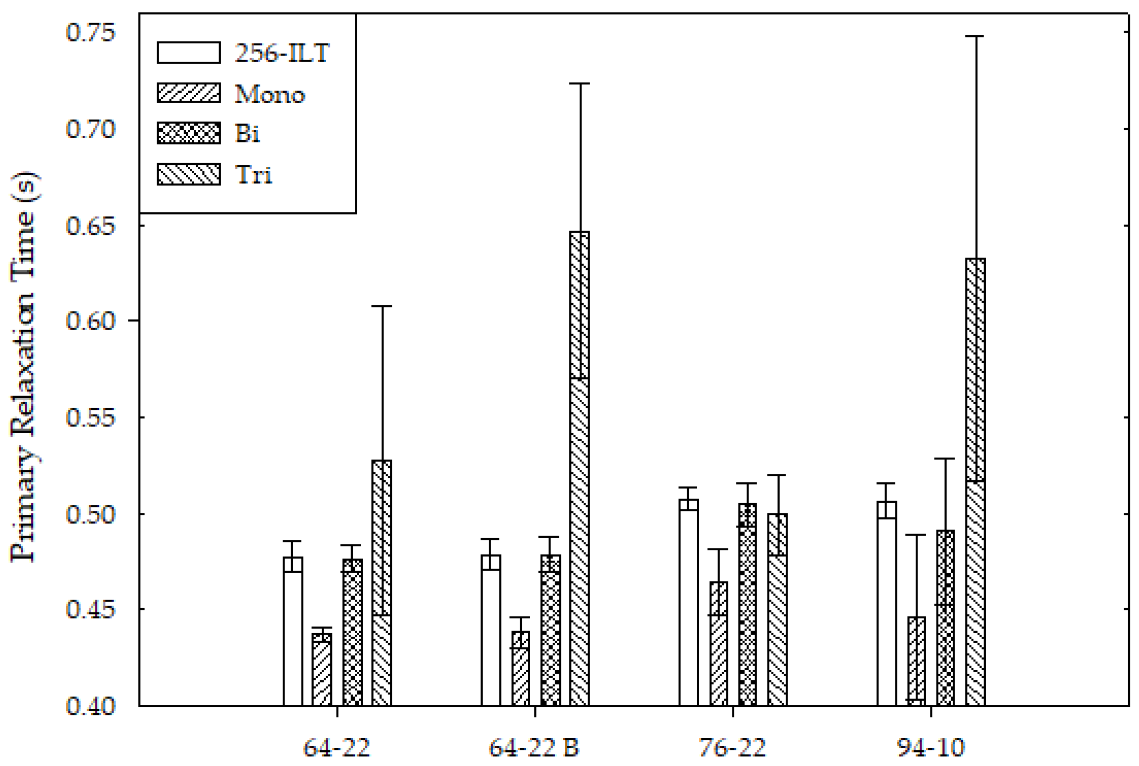
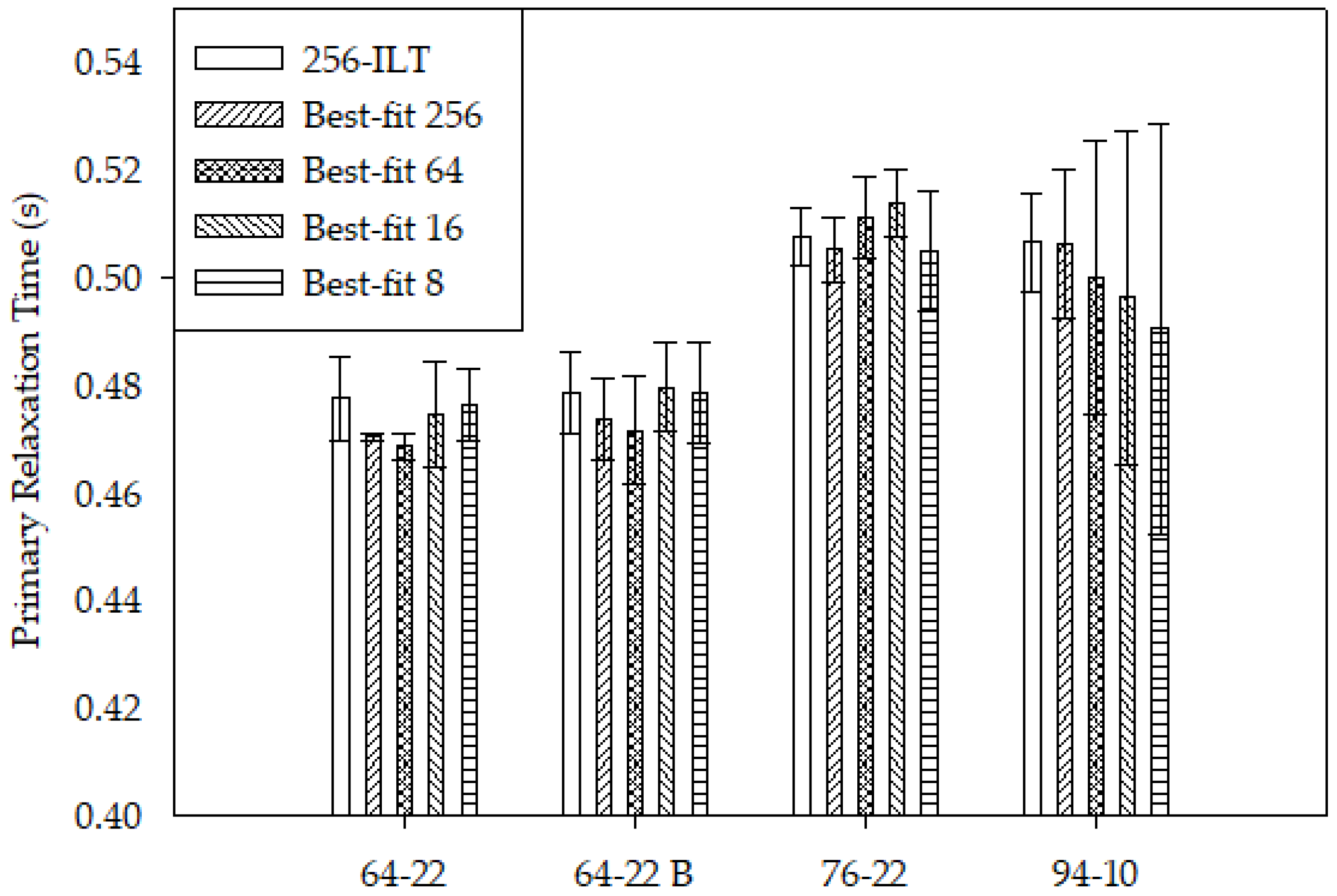
To reduce analysis time, the acquisition time must be reduced, but to differentiate binders, a comparable fit must be used. Since the best fit was determined to be biexponential, the number of data points was then decreased for comparison, as seen in
Figure 4 and
Figure 5.
Figure 4 indicates how decreasing the number of data points impacts comparability. Since the ILT is commonly considered the best fit, the accuracy of each fit could be compared. Reducing the number of data points of the PG 64-22 binders and the PG 76-22 resulted in slight fluctuations in the standard deviation. As the number of data points was reduced for the PG 94-10 sample, the standard deviation continued to increase. This clearly shows how additional data is needed for the 94-10 sample, indicating that multiple hydrogen environments exist that cannot be fit as well with less data.
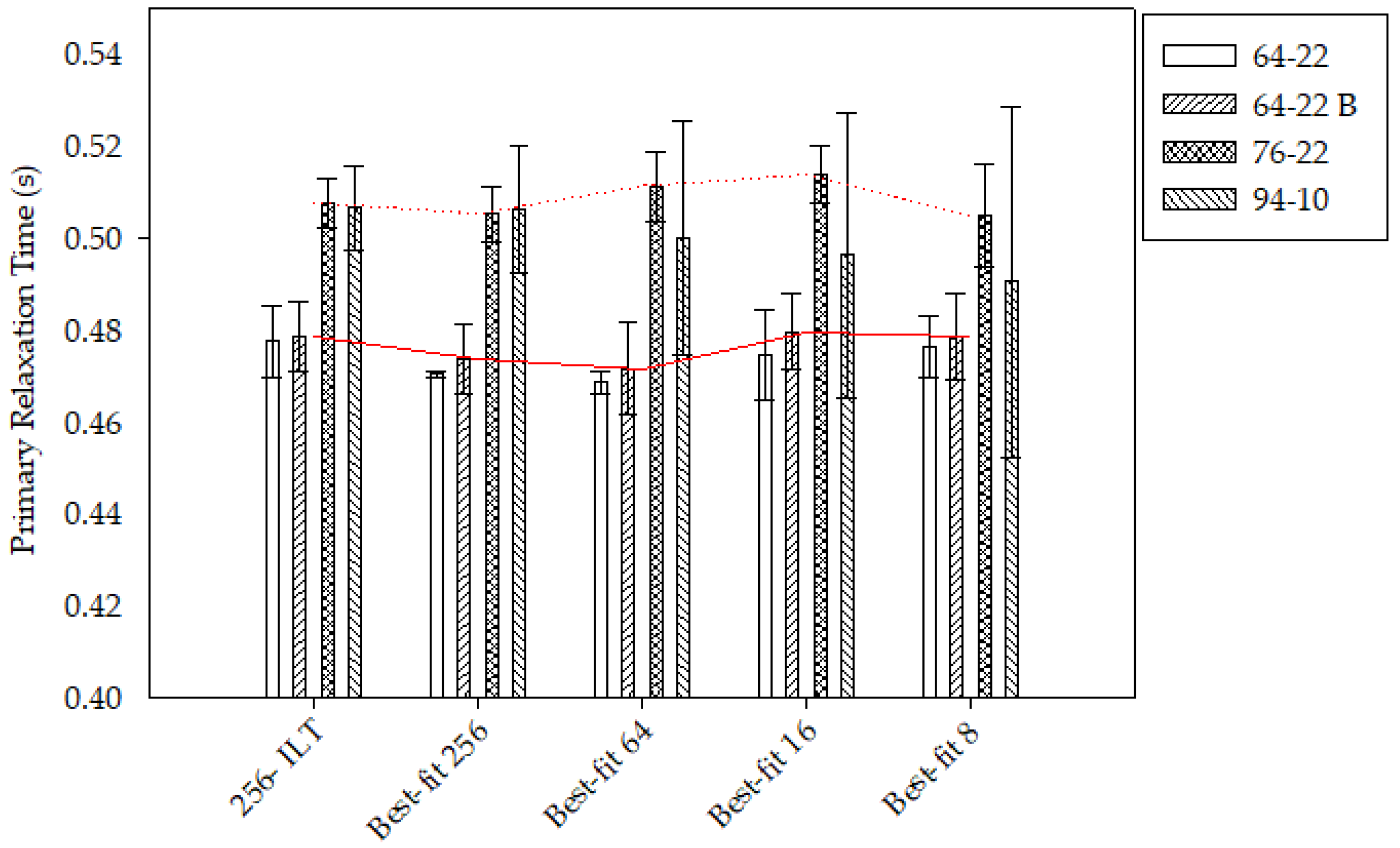
Figure 5 compares the number of data points across the binders. The general trend, shown in red, indicates that the PG 64-22 sources were comparable while the 76-22 and 94-10 were comparable with slight differences. While the PG 64-22 samples could be clearly differentiated from the PG 76-22 samples, none of the fits could differentiate the PG 76-22 from the 94-10.
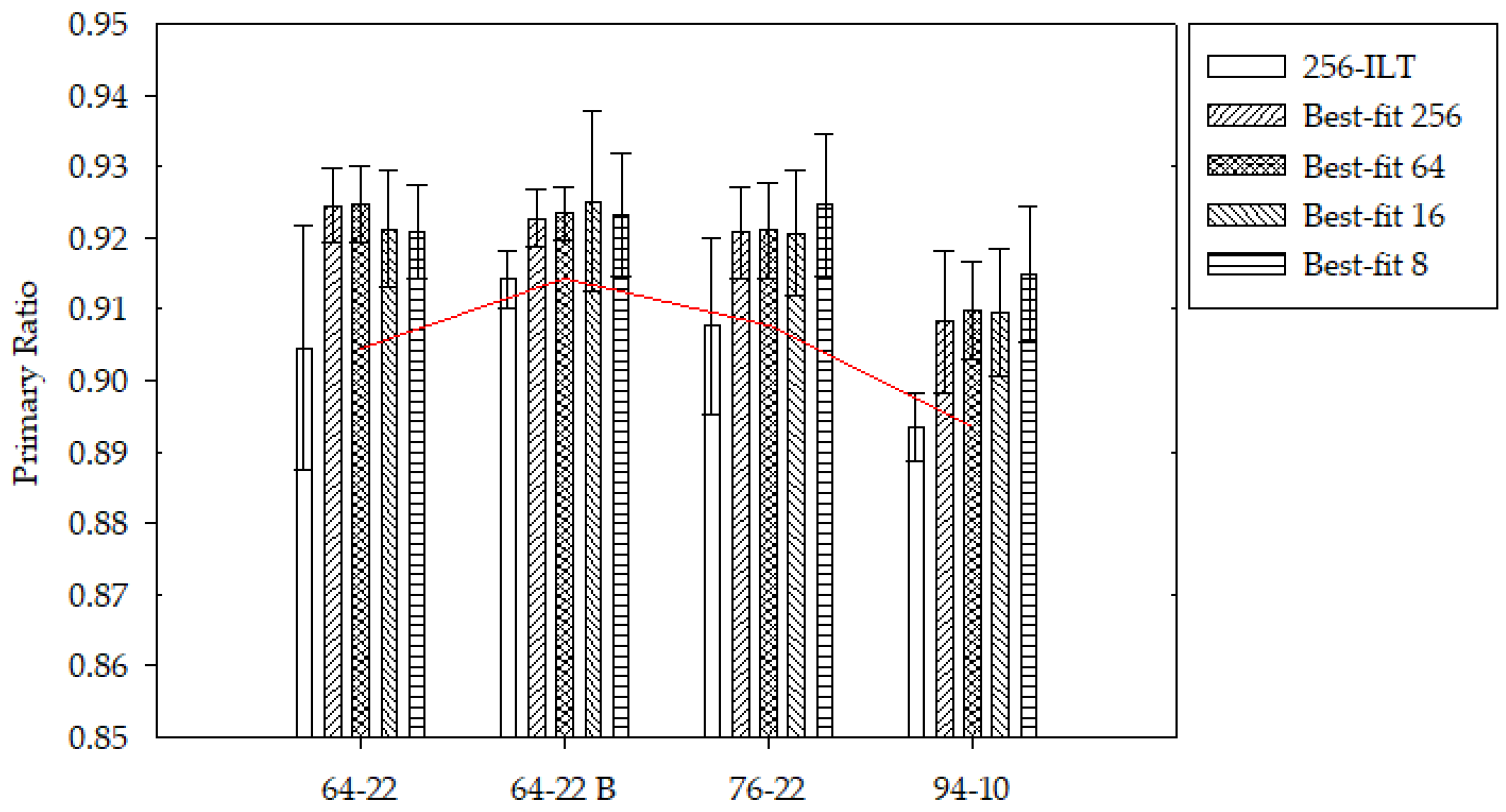
3.5. Best and Fastest T1 Ratios
By comparing the primary relaxation time, the PG 64-22 binders could be differentiated from the 76-22 binder, but not the 94-10. Therefore, another parameter must be considered. The relative ratio of the primary relaxation time for each binder, the primary ratio, was determined. While this parameter is not entirely effective in differentiating the PG 76-22 from the 94-10, it is a better estimate than just the relaxation time. This comparison is seen in
Figure 6. While the PG 64-22 and 76-22 samples had similar primary ratios, the primary ratio of the PG 94-10 sample was consistently lower than the other samples, as indicated by the general trend (red line) in
Figure 7. The primary ratio is an indication of the number of distinct hydrogen environments present. The ILT considers the highest number of hydrogen environments, while the other fits consider two due to the biexponential fit. In both analyses, there can be a lot of variability in the hydrogen environments between samples.
The number of data points also impacted the variability in the samples, as displayed in
Figure 7. Both samples of the PG 64-22 and the one sample of PG 76-22 experienced less variability when 256 and 64 data points were considered. Alternatively, the PG 94-10 displayed less variability when the inverse Laplace transform was used with 256 data points. While the ILT included more noise in the other samples, there may be more signal for the ILT to catch in the PG 94-10 samples. This is further supported due to the increase in variability and the decrease in overlap with the ILT as fewer data points were considered.
4. Discussion
4.1. Noise and Goodness of Fit
The differentiation of asphalt binders by NMR relaxometry depends on the noise, the type of fit, and the number of data points needed. The best mathematical fit of all samples would be the ILT. This mathematical iterative procedure will find the best match to the experimental data. However, since the data are noisy, some fitted relaxation times may not actually exist or be helpful. Therefore, this testing relied mainly on the most distinct relaxation time, the primary relaxation time.
The noise from the device was not a large component in the differences seen in the relaxation times of asphalt binders. When comparing the number of exponential fits, analysis indicated that a monoexponential fit is suboptimal, as shown by high X
2 values, suggesting a poor representation of the data. In contrast, a biexponential fit substantially improves the model’s accuracy, evident from significantly lower X
2 values and clearer alignment with the observed data, as seen in
Appendix A. While the triexponential fit provided a similar goodness-of-fit, as evidenced by comparable X
2 values, the additional complexity does not greatly enhance the model’s performance. Therefore, the biexponential fit is preferred for the comparison of the primary relaxation time and ratio.
4.2. Best and Fastest Comparison (T1 and Ratios)
It was shown that the type of fit and number of data points acquired did impact the primary relaxation time as well as the relative ratio, but to a lesser degree. Most of the samples had a smaller standard deviation with the mono-, bi-, or triexponential fits, not the ILT. This is occurring due to the averaging of the additional relaxation times that are resolved from the ILT. A monoexponential fit must summarize all noise into one relaxation time, so the most influential times will have the greatest impact, reducing the impact of noise. The number of relaxation times that can be resolved depends on the number of data points available. Three relaxation times is the maximum number of times that can be determined with eight data points with little confidence. While PG 64-22 and 76-22 could be differentiated, the 94-10 falls into the ranges of the other grades. Further testing should determine the best location of the data points since equally log-spaced data did not represent the data well, resulting in larger standard deviations of both the primary relaxation time and ratio.
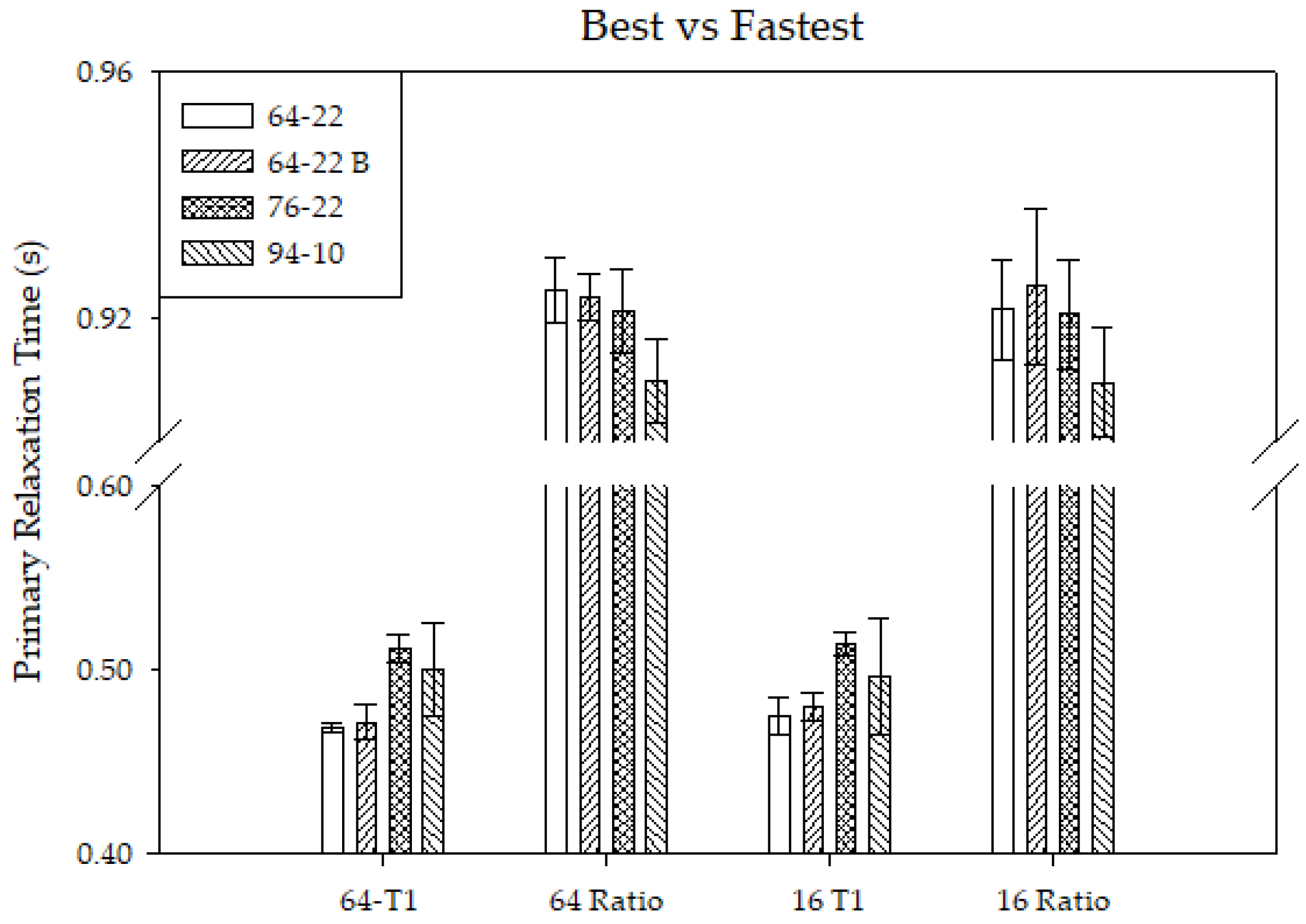
At least a biexponential is needed to consider the relative ratio, which is needed to differentiate the PG 76-22 from the 94-10. Therefore, a biexponential fit of 64 or 16 acquired points can indicate binder grades, as seen in
Figure 8. This is consistent with previous findings of asphalt that utilized a biexponential fit [
20]. The best comparison requires 64 points since the ratios between the PG 76-22 and 94-10 have the least overlap.
The major difference between binder grades is the stiffness of each binder. Since the process of assigning grades is standard, it is assumed that the PG 64-22 had the lowest viscosity, while the PG 94-10 had the largest. The idea that increased stiffness leads to longer relaxation times [
16,
17] is somewhat supported by this study. The relaxation time increased from the PG 64-22 to 76-22 but then decreased in the PG 94-10 samples. This anomaly can be explained by the decrease in the primary ratio seen in the PG 94-10 samples. Since the primary ratio decreased, more distinct hydrogen environments are present at faster relaxation times, reducing the primary relaxation time. Therefore, both the primary relaxation time and ratio are needed to differentiate asphalt binders.
5. Conclusions
The asphalt binder is a major design consideration for essential infrastructure. In differentiating asphalt binders, it takes considerable time and energy to simulate failure conditions. Chemical testing has been considered for binder characterization, but often requires intense or destructive analysis. NMR relaxometry is emerging as a potential tool for asphalt performance determination. This study concludes that asphalt binders can be differentiated using NMR analysis, but the degree of this differentiation depends on the number of data points used and the type of fit. The best mathematical fit is the ILT, but across samples, this fit was not as effective in differentiating samples since the standard deviation was very high. While the variability between samples can be high (i.e., high standard deviation), the primary relaxation time and ratio were effective in differentiating the binders. The most comparable fit with a reliable amount of data points was a biexponential fit of 64 data points. This analysis method would reduce the testing time from 214 to 50 min.
Further testing should determine the best location for fewer data points to be considered. Additionally, other parameters should be developed to describe NMR data as a powerful tool for engineering use.
Author Contributions
Conceptualization, R.M.H.; methodology, R.M.H. and K.W.; formal analysis, R.M.H. and K.L.; writing—original draft preparation, R.M.H. and K.L.; writing—review and editing, R.M.H., K.W. and M.A. All authors have read and agreed to the published version of the manuscript.
Funding
This research received no external funding.
Data Availability Statement
The dataset is available on request from the authors.
Acknowledgments
The authors would like to acknowledge both the Missouri S&T Chemistry and Civil Engineering departments for this collaborative effort. The Missouri S&T Institute for Applied NMR Spectroscopy also played a role in providing supplies and materials for this study.
Conflicts of Interest
The authors declare no conflicts of interest.
Appendix A
Figure A1.
Mathematical fits of binder types using 256 points with the general data trends in red.
Figure A1.
Mathematical fits of binder types using 256 points with the general data trends in red.
Figure A2.
Mathematical fits of binder types using 64 points.
Figure A2.
Mathematical fits of binder types using 64 points.
Figure A3.
Mathematical fits of binder types using 16 points.
Figure A3.
Mathematical fits of binder types using 16 points.
Figure A4.
Mathematical fits of binder types using eight points.
Figure A4.
Mathematical fits of binder types using eight points.
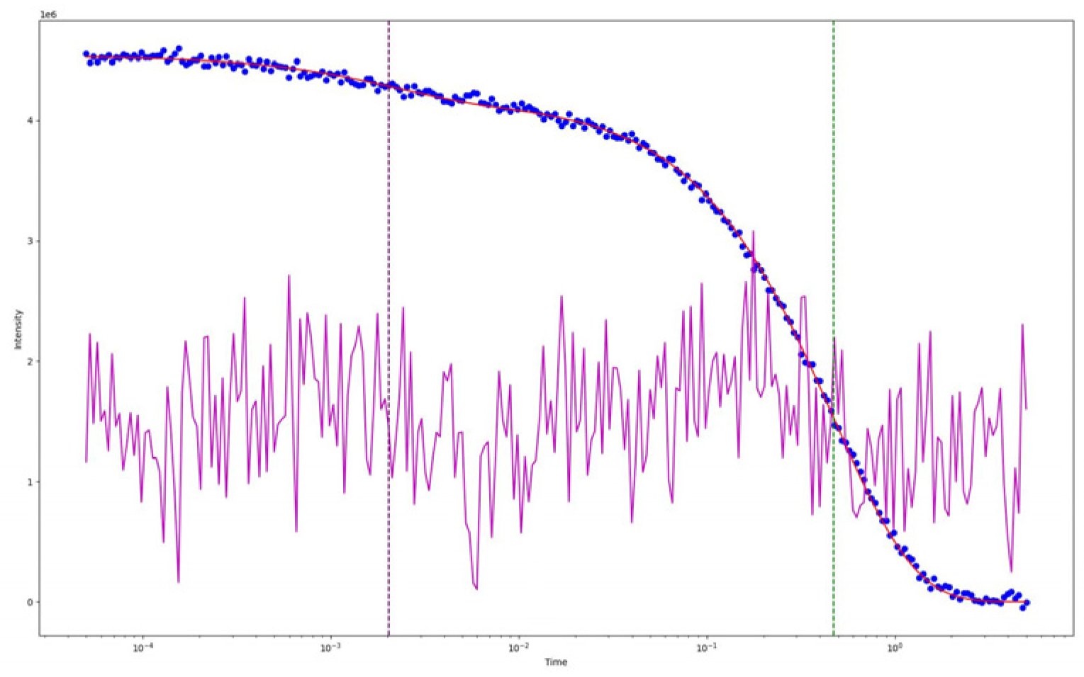
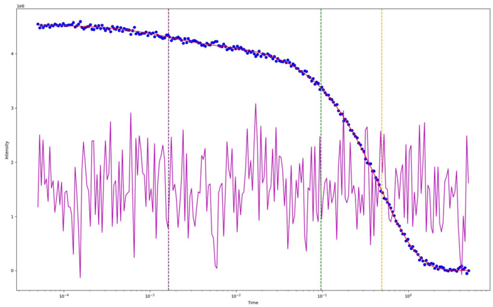
In
Figure A5 through
Figure A7, the blue points represent the experimental data, the orange curve represents the fitted curve, the vertical lines represents the fitted
T1 value, the and the purple curve represents the difference of squares. In
Figure A5, we can see the error curve increasing when the fitted curve dips below or above the experimental data. In
Figure A6, we can see that the error curve is constant across the entire time domain. This indicates a good fit. In
Figure A7, the triexponential fit produces two
T1 values on either side of the inflection point indicating overfitting of the data.
Figure A5.
A monoexponential fit of 256 data points of 64-22. The blue points represent the experimental data, the orange curve represents the fitted curve, the vertical lines rep-resents the fitted T1 value, the and the purple curve represents the difference of squares.
Figure A5.
A monoexponential fit of 256 data points of 64-22. The blue points represent the experimental data, the orange curve represents the fitted curve, the vertical lines rep-resents the fitted T1 value, the and the purple curve represents the difference of squares.
Figure A6.
A biexponential fit of 256 data points of 64-22. The blue points represent the experimental data, the orange curve represents the fitted curve, the vertical lines rep-resents the fitted T1 value, the and the purple curve represents the difference of squares.
Figure A6.
A biexponential fit of 256 data points of 64-22. The blue points represent the experimental data, the orange curve represents the fitted curve, the vertical lines rep-resents the fitted T1 value, the and the purple curve represents the difference of squares.
Figure A7.
A triexponential fit of 256 data points of 64-22. The blue points represent the experimental data, the orange curve represents the fitted curve, the vertical lines rep-resents the fitted T1 value, the and the purple curve represents the difference of squares.
Figure A7.
A triexponential fit of 256 data points of 64-22. The blue points represent the experimental data, the orange curve represents the fitted curve, the vertical lines rep-resents the fitted T1 value, the and the purple curve represents the difference of squares.
Figure A8.
Average least squares between a monoexponential, biexponential, and triexponential fit for 64 data points.
Figure A8.
Average least squares between a monoexponential, biexponential, and triexponential fit for 64 data points.
Figure A9.
Average least squares between a monoexponential, biexponential, and triexponential fit for 16 data points.
Figure A9.
Average least squares between a monoexponential, biexponential, and triexponential fit for 16 data points.
Figure A10.
Average least squares between a monoexponential, biexponential, and triexponential fit for 8 data points.
Figure A10.
Average least squares between a monoexponential, biexponential, and triexponential fit for 8 data points.
References
- Kovaľaková, M.; Fričová, O.; Hronský, V.; Olčák, D.; Mandula, J.; Salaiová, B. Characterisation of Crumb Rubber Modifier Using Solid-State Nuclear Magnetic Resonance Spectroscopy. Road Mater. Pavement Des. 2013, 14, 946–958. [Google Scholar] [CrossRef]
- Chimanowsky, J.P., Jr.; Dutra Filho, J.C.; Tavares, M.I.B. Nuclear Magnetic Resonance as a Powerful Tool for Evaluation of Intermolecular Interaction: Correlation with Rheological Measurements of Recycled Nanocomposite. Polym. Test. 2017, 63, 417–426. [Google Scholar] [CrossRef]
- Kuhn, W. NMR Microscopy—Fundamentals, Limits and Possible Applications. Angew. Chem. Int. Ed. Engl. 1990, 29, 1–19. [Google Scholar] [CrossRef]
- Fiilber, C.; Demco, D.E.; Weintraub, O.; Bliimich, B. The Effect of Crosslinking in Elastomers Investigated by NMR Analysis of 13C Edited Transverse 1H NMR Relaxation. Macromol. Chem. Phys. 1996, 197, 581–593. [Google Scholar] [CrossRef]
- Wang, M.; Bertmer, M.; Demco, D.E.; Blu, B. Segmental and Local Chain Mobilities in Elastomers by 13C-1H Residual Heteronuclear Dipolar Couplings. J. Phys. Chem. B 2004, 108, 10911–10918. [Google Scholar] [CrossRef]
- Spiess, H.W. Rotation of Molecules and Nuclear Spin Relaxation. In Dynamic NMR Spectroscopy; Springer: Berlin/Heidelberg, Germany, 1978. [Google Scholar]
- Bliimler, P.; Blumich, B. Aging and Phase Separation of Elastomers Investigated by NMR Imaging. Macromolecules 1991, 24, 2183–2188. [Google Scholar] [CrossRef]
- Klinkenberg, M.; Blu, P.; Blu, B. 2H-NMR Imaging of Stress in Strained Elastomers. Macromolecules 1997, 30, 1038–1043. [Google Scholar] [CrossRef]
- Blümler, P.; Blümich, B. NMR Imaging of Elastomers: A Review. Rubber Chem. Technol. 1997, 70, 468–518. [Google Scholar] [CrossRef]
- Berlin, S.-V.; New, H.; London, Y.; Tokyo, P.; Kong, H. Nondestructive Characterization of Materials. In Proceedings of the 3rd International Symposium, Saarbrücken, Germany, 3–6 October 1988. [Google Scholar]
- Caputo, P.; Loise, V.; Ashimova, S.; Teltayev, B.; Vaiana, R.; Oliviero Rossi, C. Inverse Laplace Transform (ILT)NMR: A Powerful Tool to Differentiate a Real Rejuvenator and a Softener of Aged Bitumen. Colloids Surf. A Physicochem. Eng. Asp. 2019, 574, 154–161. [Google Scholar] [CrossRef]
- Filippelli, L.; Rossi, C.O.; Carini, M.; Chiaravalloti, F.; Gentile, L. Structural Characterization of Bitumen System by Prony-like Method Applied to NMR and Rheological Relaxation Data. Mol. Cryst. Liq. Cryst. 2013, 572, 50–58. [Google Scholar] [CrossRef]
- Evdokimov, I.N.; Eliseev, N.Y.; Akhmetov, B.R. Asphaltene Dispersions in Dilute Oil Solutions. Fuel 2006, 85, 1465–1472. [Google Scholar] [CrossRef]
- Jaimes, M.L.; Santos, S.N.; Molina, V.D. Prediction of the Penetration Grade and Softening Point of Vacuum Residues and Asphalts by Nuclear Magnetic Resonance and Chemometric Methods. Energy Fuels 2019, 33, 6264–6272. [Google Scholar] [CrossRef]
- Blümich, B. Aging of Polymeric Materials by Stray-Field NMR Relaxometry with the NMR-MOUSE. Concepts Magn. Reson. Part A 2018, 47, e21464. [Google Scholar] [CrossRef]
- Herndon, R.M.; Balasubramanian, J.; Woelk, K.; Abdelrahman, M. Physical and Chemical Methods to Assess Performance of TPO-Modified Asphalt Binder. Appl. Sci. 2024, 14, 3300. [Google Scholar] [CrossRef]
- Herndon, R.; Balasubramanian, J.; Woelk, K.; Abdelrahman, M. Investigating the Physical and Chemical Effects of UV Aging on TPO-Modified Asphalt Binder. In Modern Concepts in Material Science; Iris Publishers: San Francisco, CA, USA, 2024. [Google Scholar]
- Herndon, R.M.; Balasubramanian, J.; Abdelrahman, M.; Woelk, K. Nuclear Magnetic Resonance (NMR) Assessment of Bio and Crude Oil-Based Rejuvenation. Physchem 2024, 4, 344–355. [Google Scholar] [CrossRef]
- Herndon, R.M.; Balasubramanian, J.; Abdelrahman, M.; Woelk, K. Asphalt-Binder Mixtures Evaluated by T1 NMR Relaxometry. Physchem 2024, 4, 285–295. [Google Scholar] [CrossRef]
- Blümich, B.; Teymouri, Y.; Clark, R. NMR on the Road: Non-Destructive Characterization of the Crumb-Rubber Fraction in Asphalt. Appl. Magn. Reson. 2019, 50, 497–509. [Google Scholar] [CrossRef]
- Bro, R.; Sidiropoulos, N.D.; Smilde, A.K. Maximum Likelihood Fitting Using Ordinary Least Squares Algorithms. J. Chemom. 2002, 16, 387–400. [Google Scholar] [CrossRef]
- Mayes, Z.G.; Rice, W.H.; Chi, L.; Woelk, K. A Robust Freeman-Hill-Inspired Pulse Protocol for Ringdown-Free T1 Relaxation Measurements. J. Magn. Reson. 2023, 352, 107490. [Google Scholar] [CrossRef]
- Filippelli, L.; Gentile, L.; Rossi, C.O.; Ranieri, G.A.; Antunes, F.E. Structural Change of Bitumen in the Recycling Process by Using Rheology and NMR. Ind. Eng. Chem. Res. 2012, 51, 16346–16353. [Google Scholar] [CrossRef]
- Gentile, L.; Filippelli, L.; Rossi, C.O.; Baldino, N.; Ranieri, G.A. Rheological and 1H-NMR Spin-Spin Relaxation Time for the Evaluation of the Effects of PPA Addition on Bitumen. Mol. Cryst. Liq. Cryst. 2012, 558, 54–63. [Google Scholar] [CrossRef]
| Disclaimer/Publisher’s Note: The statements, opinions and data contained in all publications are solely those of the individual author(s) and contributor(s) and not of MDPI and/or the editor(s). MDPI and/or the editor(s) disclaim responsibility for any injury to people or property resulting from any ideas, methods, instructions or products referred to in the content. |
© 2024 by the authors. Licensee MDPI, Basel, Switzerland. This article is an open access article distributed under the terms and conditions of the Creative Commons Attribution (CC BY) license (https://creativecommons.org/licenses/by/4.0/).


