Thermodynamic Analysis of Ar_xXe_1-x Solid Solutions Based on Kirkwood–Buff Theory

Abstract

Kirkwood–Buff Integral (KBI) theory is an important method for the analysis of the structural and thermodynamic properties of liquid solutions. For solids, the calculation of KBIs has become possible only recently through the finite-volume generalisation of KBI theory, but it has so far only been applied to monoatomic crystals. Here, we show that KBI theory can be applied to solid mixtures and compute the KBIs of a Ar${}_x$Xe${}_{1-x}$ solid solution, for $0<x<0.1$ and temperature $T=84-86$ K, from pair distribution functions obtained by Monte Carlo simulation. From the KBIs, the isothermal compressibility, partial molar volumes, and thermodynamic factors are calculated and found to be in good agreement with alternative theoretical methods. The analysis of the KBIs and the partial molar volumes give insight into the structure of the mixture. The KBI of Ar pairs is much larger than that of Xe pairs, which indicates the tendency of Ar impurities to accumulate. The evolution of the partial molar volumes with increasing Ar molar fraction x shows a transition at $x\approx 0.06$, which reflects the formation of Ar clusters, precursors of the Ar-rich liquid phase. The calculated thermodynamic factors show that the solid(Xe) phase becomes unstable at $x\approx 0.1$, indicating the start of the solid (Xe)–liquid (Ar) equilibrium. The chemical potentials of Ar and Xe are obtained from the thermodynamic factor by integration over $lnx$, and by fitting the data to the Margules equations, the activity coefficients can be estimated over the whole composition range. The present findings extend the domain of applicability of the KBI solution theory from liquids to solids.

1. Introduction

Kirkwood–Buff Integral (KBI) theory [1], is considered to be one of the most important theories of solutions [2], because it relies only on general, exact relations of statistical mechanics. A KBI is a simple volume integral over the Radial pair Distribution Function (RDF). In a mixture with N species, there are $N(N-1)/2$ independent RDFs and, thus, as many independent KBIs. These KBIs are directly related to the particle number fluctuations. From the latter, various thermodynamic quantities can be obtained, including the compressibility, partial molar volumes, and the thermodynamic factor $\Gamma$, i.e., the derivative of the chemical potential with molar fraction [2], which is a key quantity for computing diffusion coefficients [3,4]. KBI theory is widely used in the study of liquid mixtures and solutions, either for obtaining thermodynamic quantities from molecular simulation [5,6,7,8] or, inversely, by extracting the KBIs, which contain structural information, from measured thermodynamic quantities (so-called “inverse KBI” [2,9]). In the last decade, there have been many methodological advances in KBI theory, which have substantially improved the efficiency and accuracy of KBIs for thermodynamic modelling of liquids; see, e.g., [10] for a review, where the reader may find a detailed introduction to finite-volume Kirkwood–Buff theory, used here. KBI theory was originally formulated for liquid mixtures. However, since KBI theory relies only on general statistical mechanics, it should also be useful for the study of solids. The only ingredient of KBI theory is the RDF, which is available from simulation or diffraction experiments in all kinds of matter, including liquids, granular matter, glasses, and crystalline solids [11,12]. However, to the best of our knowledge, KBI theory has never been applied to solid mixtures. The standard KBI technique cannot be used in solids, because the usual, “running” KBI diverges, reflecting the long-range correlations between the atomic positions in a crystal. This problem has recently been overcome by Miyaji et al. [13] and Krüger [14], who showed that in crystals, the KBIs do converge, provided that the generalisation of KBI theory to finite volumes [15] is used. Miyaji et al. [13] also introduced a convolution of the RDF, which dramatically accelerates the convergence of the KBI with system size. By combining the finite-volume KBI and the convolution of the RDF, the KBI of solid argon could be calculated accurately from MC simulations on a few thousand atoms. For $T=0$ K, the exact KBI value was obtained within 0.05%, and for finite temperatures, the KBI values converged to 1% or better. The isothermal compressibility obtained from the KBI underestimates the experimental values by about 40% independently of temperature. The error was corrected based on a simple mechanical calculation valid at $T=0$ K, and the corrected values were in good agreement with the experiment in the whole temperature range of the solid phase ($0<T<80$ K). After having shown that KBI theory can be applied to solids [13,14], we now turn to the main purpose of the KBI method, namely the study of solutions.

In this paper, we present the first application of KBI theory to a solid mixture, namely the Ar${}_x$Xe${}_{1-x}$ solid solution at temperatures 84–86 K. For the Ar-Xe mixture in this temperature range, accurate thermodynamic data are lacking. According to an approximate Ar-Xe phase diagram [16], the system is a Xe-rich solid for an Ar concentration x below about 5%, an Ar-rich liquid for x above about 80%, and in the solid–liquid equilibrium for x between these two values. We focus on the range $0<x<0.1$, i.e., the Xe-rich solid solution. The KBIs are obtained from MC simulations by using the finite-volume KBI theory and the convolution of the RDF [13]. We find, as in the case of monoatomic crystals [13], that KBI theory considerably underestimates the isothermal compressibility. The Ar and Xe partial molar volumes, however, agree very well with the values obtained by a standard theoretical method. The partial molar volumes display a weak, linear variation with x for $x<0.06$. For higher Ar concentrations, the partial molar volume of Ar strongly decreases, which indicates a transition from the solid solution phase to a solid–liquid equilibrium, in agreement with the phase diagram [16]. The phase change is also indicated by the formation of Ar clusters and by the evolution of the affinity coefficients, which are computed from the KBI and the Margules equations. The present results show that KBI theory can be applied to solid mixtures, and partial molar volumes and activity coefficients can be obtained from the KBIs. This is a key step in the effort to extend KBI theory to a general technique for the thermodynamic analysis of multicomponent condensed matter systems.

2. Materials and Methods

2.1. Theory

2.1.1. Kirkwood–Buff Integrals in Crystals

In a mixture containing species $\alpha$, $\beta$, …, the Pair Distribution Function (PDF) $g_{\alpha \beta }(\mathbf{r},{\mathbf{r}}^{\prime })$ is defined by

$$g_{\alpha \beta }\left(\mathbf{r},{\mathbf{r}}^{\prime }\right)=\frac{\langle {\sum }_{i_{\alpha }\ne j_{\alpha }}\delta \left({\mathbf{R}}_{i_{\alpha }}-\mathbf{r}\right)\delta \left({\mathbf{R}}_{j_{\beta }}-{\mathbf{r}}^{\prime }\right)\rangle }{{\rho }_{\alpha }\left(\mathbf{r}\right){\rho }_{\beta }\left({\mathbf{r}}^{\prime }\right)}$$

(1)

where ${\mathbf{R}}_{i_{\alpha }}$ is the position of particle i of atomic species $\alpha$, $\langle \dots \rangle$ denotes the statistical average, and ${\rho }_{\alpha }\left(\mathbf{r}\right)=\langle {\sum }_{i_{\alpha }}\delta \left({\mathbf{r}}_{i_{\alpha }}-\mathbf{r}\right)\rangle =N_{\alpha }/V$ is the single-particle density. $N_{\alpha }$ is the number of $\alpha$-particles in the volume V. For the statistical averages, we assume, as in our previous applications of KBI theory to solids [13,17], that the macroscopic system is isotropic and homogeneous, i.e., it has the symmetry of a liquid. This may be justified by considering a powder sample, which is an ensemble of crystals of arbitrary origin and orientation [17]. In this ensemble, the partial densities are constant, ${\rho }_{\alpha }\left(\mathbf{r}\right)={\rho }_{\alpha }$, and the PDF depends only on the particle distance $r=|\mathbf{r}-{\mathbf{r}}^{\prime }|$, i.e., it becomes an RDF, denoted $g_{\alpha \beta }\left(r\right)$. The usual, “running” KBI is given by

$$G_{\alpha \beta }^{\mathrm{R}}\left(L\right)={\int }_0^L(g_{\alpha \beta }\left(r\right)-1)4\pi r^{2}dr.$$

(2)

where L is a cutoff radius. The finite-volume KBI is defined as [15]

$$G_{\alpha \beta }^V=\frac{1}{V}{\int }_{V}d{\mathbf{r}}_1{\int }_{V}d{\mathbf{r}}_2(g_{\alpha \beta }\left(r\right)-1),$$

(3)

where $r=|{\mathbf{r}}_1-{\mathbf{r}}_2|$. It can be rewritten exactly as [15,18]

$$G_{\alpha \beta }^{\mathrm{F}}\left(L\right)\equiv G_{\alpha \beta }^V={\int }_0^L(g_{\alpha \beta }\left(r\right)-1)y(r/L)4\pi r^{2}dr,$$

(4)

where L is the maximum distance in V. $y\left(x\right)$ is a geometrical function, which only depends on the shape of V [19,20]. For a sphere of diameter L, we have

$$y\left(x\right)=1-3x/2+x^3/2.$$

(5)

To accelerate the convergence of the finite-volume KBI, several expressions have been proposed [15,19,21]. In this study, we use the second-order extrapolation by Krüger and Vlugt [19]. It is obtained from Equation (4) upon replacing $y\left(x\right)$ with $y_2\left(x\right)$, given by

$$y_2\left(x\right)=1+(-23x^3+6x^4+9x^5)/8;$$

(6)

thus,

$$G_{\alpha \beta }\left(L\right)={\int }_0^L(g_{\alpha \beta }\left(r\right)-1)y_2(r/L)4\pi r^{2}dr.$$

(7)

A two-component system with species A and B has three independent RDFs $g_{\mathrm{AA}}$, $g_{\mathrm{BB}}$, and $g_{\mathrm{AB}}$ and three corresponding infinite-volume KBIs, $G_{\mathrm{AA}}^{\infty }$, $G_{\mathrm{BB}}^{\infty }$, and $G_{\mathrm{AB}}^{\infty }$. They are related to the partial molar volume of atom A, ${\overline{V}}_{\mathrm{A}}$, isothermal compressibility ${\kappa }_T$, and thermodynamic correction factor $\Gamma$, the derivative of the chemical potential of a species with its molar fraction, by [1]

$$\begin{array}{cc}\hfill {\overline{V}}_{\mathrm{A}}& ={\left(\frac{\partial V}{\partial N_A}\right)}_{T,P,N_B}=\frac{1+{\rho }_{\mathrm{B}}\left(G_{\mathrm{BB}}^{\infty }-G_{\mathrm{AB}}^{\infty }\right)}{{\rho }_{\mathrm{A}}+{\rho }_{\mathrm{B}}+{\rho }_{\mathrm{A}}{\rho }_{\mathrm{B}}\left(G_{\mathrm{AA}}^{\infty }+G_{\mathrm{BB}}^{\infty }-2G_{\mathrm{AB}}^{\infty }\right)},\hfill \end{array}$$

(8)

$$\begin{array}{cc}\hfill {\kappa }_T& =-\frac{1}{V}{\left(\frac{\partial V}{\partial P}\right)}_T=\frac{1+{\rho }_{\mathrm{A}}{G}_{\mathrm{AA}}^{\infty }+{\rho }_{\mathrm{B}}{G}_{\mathrm{BB}}^{\infty }+{\rho }_{\mathrm{A}}{\rho }_{\mathrm{B}}\left(G_{\mathrm{AA}}^{\infty }{G}_{\mathrm{BB}}^{\infty }-G_{\mathrm{AB}}^{\infty 2}\right)}{kT\left({\rho }_{\mathrm{A}}+{\rho }_{\mathrm{B}}+{\rho }_{\mathrm{A}}{\rho }_{\mathrm{B}}\left(G_{\mathrm{AA}}^{\infty }+G_{\mathrm{BB}}^{\infty }-2G_{\mathrm{AB}}^{\infty }\right)\right)},\hfill \end{array}$$

(9)

$$\begin{array}{cc}\hfill \Gamma & =\frac{x_{\mathrm{A}}}{kT}{\left(\frac{\partial {\mu }_{\mathrm{A}}}{\partial x_{\mathrm{A}}}\right)}_{T,P}=\frac{({\rho }_{\mathrm{A}}+{\rho }_{\mathrm{B}})}{\left[{\rho }_{\mathrm{A}}+{\rho }_{\mathrm{B}}+{\rho }_{\mathrm{A}}{\rho }_{\mathrm{B}}\left(G_{\mathrm{AA}}+G_{\mathrm{BB}}-2G_{\mathrm{AB}}\right)\right]},\hfill \end{array}$$

(10)

where T is the temperature, k is the Boltzmann constant, and P is the pressure.

2.1.2. Convolution of the RDF

In order to reduce the oscillations of the KBI and accelerate its convergence to the infinite-volume limit $G_{\alpha \beta }^{\infty }$, we use a convolution of the RDF, which leaves $G_{\alpha \beta }^{\infty }$ invariant [13]. It is based on a modified PDF where the 3D delta-functions in Equation (1) are replaced by

$$\Delta \left(\mathbf{r}\right)=\left\{\begin{array}{cc}6/\left(\pi {\sigma }^3\right)\hfill & \mathrm{if}\left|\mathbf{r}\right|<\sigma /2\hfill \\ 0\hfill & \mathrm{otherwise}\hfill \end{array}\right.$$

(11)

where $\sigma$ is the peak width. The original PDF is recovered in the limit $\sigma \to 0$. Physically, the modification $\delta \left(\mathbf{r}\right)\to \Delta \left(\mathbf{r}\right)$ amounts to replacing point-like particles, corresponding to the centre of mass of the atoms, by spherical particles of constant density. In a homogeneous, isotropic system, the modified PDF reduces to an RDF $\tilde{g}\left(r\right)$, which can be written as a convolution of the original RDF $g\left(r\right)$, i.e.,

$$\tilde{g}\left(r\right)=\int g\left(r^{\prime }\right)\chi (r^{\prime },r)d{r}^{\prime },$$

(12)

where $\chi (r^{\prime },r)$ is given by [13]

$$\chi (x^{\prime },x)=6{x^{\prime }}^2[2{\xi }_0(x^{\prime },x)-3{\xi }_1(x^{\prime },x)+{\xi }_3(x^{\prime },x)]$$

(13)

with

$${\xi }_n(x,x^{\prime })=\frac{{\left[\min (1,x+x^{\prime })\right]}^{n+2}-{|x-x^{\prime }|}^{n+2}}{(n+2)x{x}^{\prime }}.$$

(14)

2.1.3. RDF Correction by Ganguly and van der Vegt

KBI theory was formulated for open systems in the grand canonical ensemble [1]. For dense systems, molecular simulations are difficult in the grand canonical ensemble for numerical reasons, related to the need for particle insertion. In practice, most simulations are performed for closed systems in the canonical ensemble. In this case, the RDF must be corrected for the ensemble error before it can be used in the KBI. Several correction schemes have been proposed [6,15,22]. We use the method by Ganguly and van der Vegt [6], which was found to perform very well in comparative studies [10,18]. The corrected RDF $g_{\alpha \beta }^{\mathrm{vdV}}\left(r\right)$ is given by

$$g_{\alpha \beta }^{\mathrm{vdV}}\left(r\right)=g_{\alpha \beta }\left(r\right)\frac{N_{\beta }\left(1-V/V_{\mathrm{box}}\right)}{N_{\beta }\left(1-V/V_{\mathrm{box}}\right)-\Delta N_{\alpha \beta }\left(r\right)-{\delta }_{\alpha \beta }}.$$

(15)

where $g_{\alpha \beta }\left(r\right)$ is the original (canonical) RDF, $V_{\mathrm{box}}$ is the volume of the simulation box, $V=4\pi r^3/3$, $N_{\beta }$ is the number of $\beta$-particles in V, and $\Delta N_{\alpha \beta }\left(r\right)$ is the excess or depletion of particles $\beta$ in a sphere of radius r around a central particle $\alpha$, given by

$$\Delta N_{\alpha \beta }\left(r\right)={\int }_0^r[g_{\alpha \beta }\left(r^{\prime }\right)-1]4\pi {r\prime }^2{\rho }_{\beta }d{r}^{\prime }.$$

(16)

The correction (15) accounts for the fact that, in a closed system, the average density in the “reservoir” region ($r^{\prime }>r$) is different from the bulk density.

2.2. Monte Carlo Simulations

We performed Monte Carlo (MC) simulations for Ar-Xe mixtures at 1 atm, temperature 84–86 K, and Ar concentration $x_{\mathrm{Ar}}=$ 0–10%. For the interatomic potential, we used the Mie potential, which gave good results for various noble gas mixtures [23]. It is given by

$$U_{\mathrm{Mie}}\left(r\right)=C_n{ϵ}_{\alpha \beta }\left[{\left(\frac{{\sigma }_{\alpha \beta }}{r}\right)}^{n_{\alpha \beta }}-{\left(\frac{{\sigma }_{\alpha \beta }}{r}\right)}^6\right],$$

(17)

where $n_{\alpha \beta }=\sqrt{n_{\alpha }{n}_{\beta }}$,

$$C_n=\left(\frac{n_{\alpha \beta }}{n_{\alpha \beta }-6}\right){\left(\frac{n_{\alpha \beta }}{6}\right)}^{6/\left(n_{\alpha \beta }-6\right)},$$

(18)

and ${\sigma }_{\alpha \beta }$ and ${ϵ}_{\alpha \beta }$ are calculated by the Lorentz–Berthelot combining rules [24,25]:

$$\begin{array}{cc}\hfill {\sigma }_{\alpha \beta }& =\frac{{\sigma }_{\alpha }{\sigma }_{\beta }}{2},\hfill \end{array}$$

(19)

$$\begin{array}{cc}\hfill {ϵ}_{\alpha \beta }& =\sqrt{{ϵ}_{\alpha }{ϵ}_{\beta }}.\hfill \end{array}$$

(20)

The potential parameters are summarised in the

Table 1. Mie potential parameters used for Ar and Xe, taken from Ref. [23].

Atom	${\mathit{ϵ}}_{\mathit{\alpha }}/\mathit{k}$ (K)	${\mathit{\sigma }}_{\mathit{\alpha }}$ (Å)	${\mathit{n}}_{\mathit{i}}$
Ar	122.10	3.405	13
Xe	243.80	3.964	14

.

The cutoff radius of the potential was set to 10Å, and the tail correction [23] was applied. The simulations were performed with the DL-Monte code [26,27]. A cubic box with periodic boundary conditions was used, and the initial positions of the atoms were set to the fcc lattice points. In addition to the normal MC steps, i.e., the incremental motion of single atoms, we also included MC steps where an Ar atom and a Xe atom swap places. This is necessary for reaching thermal equilibrium in a reasonable time, because diffusion rates are extremely low in solids. The particle swaps did not lead to numerical artefacts, as we checked.

First, the density of the system was determined by simulations in the NpT ensemble of the system with a total number of 500 particles. The total number of MC steps was 150 million, of which 20 million steps were discarded as steps to reach equilibrium. The densities were sampled every 100 steps to obtain the statistical averages. In the same simulation, we calculated the isothermal compressibility from the volume fluctuations. For the Ar concentration range of 0–10%, simulations were carried out at exactly 2% intervals. Using the densities obtained in the NpT ensemble, the RDFs were calculated by MC simulations in the NVT ensemble with a total number of 4000 particles. The total number of MC steps was 840 million, of which 40 million steps were discarded as steps to reach equilibrium. The RDFs were convoluted with Equation (12), and the vdV correction (15) was applied. Then, the partial molar volumes of Ar and Xe, the isothermal compressibility and, the thermodynamic factor were obtained from the finite-volume KBI method, using Equations (7)–(10). For one temperature, $T=85$ K, the partial molar volumes were also obtained using the following, standard method. The volume V of the mixture was computed in two $NpT$ simulations, one for particle numbers ($N_{\mathrm{Ar}}$, $N_{\mathrm{Xe}}$), corresponding to $x_{\mathrm{Ar}}=0.02,0.04,\dots$, and one for either ($N_{\mathrm{Ar}}+1$, $N_{\mathrm{Xe}}-1$) or ($N_{\mathrm{Ar}}-1$, $N_{\mathrm{Xe}}+1$). Assuming ${\overline{V}}_{\mathrm{Ar}}$, ${\overline{V}}_{\mathrm{Xe}}$ constant under this small concentration variation, their values can be obtained from the relation

$$V=N_{\mathrm{Ar}}{\overline{V}}_{\mathrm{Ar}}+N_{\mathrm{Xe}}{\overline{V}}_{\mathrm{Xe}},$$

(21)

evaluated at the two ($N_{\mathrm{Ar}}$, $N_{\mathrm{Xe}}$) points. This method is equivalent to a numerical differentiation of the $V\left(x\right)$ curve.

3. Results and Discussion

3.1. Monte Carlo Simulation

The determined average density, KBIs, isothermal compressibility, and thermodynamic factor are listed in

Table 2. Equilibrium density $\rho$ and isothermal compressibility ${\kappa }_T^{\mathrm{NpT}}$ from NpT simulations as a function of temperature T and Ar concentration $x_{\mathrm{Ar}}$. KBI values $G_{\alpha \beta }$ for $\{\alpha ,\beta \}=${Ar,Xe} and derived quantities (superscript “KBI”): isothermal compressibility ${\kappa }_T$, thermodynamic correction factor $\Gamma$.

T (K)	${\mathit{x}}_{\mathbf{Ar}}$	$\mathit{\rho }$ (Å${}^{-3}$)	${\mathit{G}}_{\mathbf{ArAr}}$ (${10}^3$Å${}^3$)	${\mathit{G}}_{\mathbf{ArXe}}$ (${10}^2$Å${}^3$)	${\mathit{G}}_{\mathbf{XeXe}}$ (Å${}^3$)	${\mathit{\kappa }}_{\mathit{T}}^{\mathbf{KBI}}$ (GPa${}^{-1}$)	${\mathit{\kappa }}_{\mathit{T}}^{\mathbf{NpT}}$ (GPa${}^{-1}$)	${\mathbf{\Gamma }}^{\mathbf{KBI}}$
84	0	0.01690	-	-	−58.96	0.1950	0.2804	1.00
85	0	0.01689	-	-	−58.99	0.1960	0.2824	1.00
86	0	0.01688	-	-	−59.02	0.1973	0.2849	1.00
84	0.02	0.01694	0.7936	−0.7045	−58.68	0.2042	0.2873	0.775
85	0.02	0.01693	0.8471	−0.7092	−58.72	0.2063	0.2896	0.764
86	0.02	0.01692	0.8507	−0.7157	−58.72	0.2058	0.2930	0.763
84	0.04	0.01698	1.047	−0.9630	−57.41	0.2132	0.2967	0.565
85	0.04	0.01697	1.082	−0.9769	−57.38	0.2166	0.2981	0.557
86	0.04	0.01696	1.120	−0.9913	−57.37	0.2167	0.3014	0.549
84	0.06	0.01702	1.768	−1.602	−52.85	0.2340	0.3057	0.339
85	0.06	0.01701	1.712	−1.567	−53.11	0.2328	0.3078	0.346
86	0.06	0.01700	1.524	−1.466	−53.69	0.2335	0.3112	0.372
84	0.08	0.01707	3.430	−3.258	−37.82	0.2631	0.3134	0.165
85	0.08	0.01706	3.175	−3.055	−39.48	0.2638	0.3167	0.175
86	0.08	0.01705	2.656	−2.667	−42.43	0.2588	0.3188	0.202
84	0.10	0.01712	18.12	−18.39	116.3	0.3367	0.3250	0.0288
85	0.10	0.01711	15.50	−15.81	90.86	0.3318	0.3270	0.0335
86	0.10	0.01710	7.101	−7.597	10.54	0.3131	0.3300	0.0700

as a function of temperature and Ar concentration. The partial molar volumes are listed in

Table 3. Partial molar volumes ${\overline{V}}_{\mathrm{Ar}}$ and ${\overline{V}}_{\mathrm{Xe}}$ obtained either using KBI theory (${\overline{V}}^{\mathrm{KBI}}$) or from two NpT simulations and Equation (21) with particle numbers ($N_{\mathrm{Ar}}$, $N_{\mathrm{Xe}}$) corresponding to $x_{\mathrm{Ar}}$ and ($N_{\mathrm{Ar}}\pm 1$, $N_{\mathrm{Xe}}\mp 1$). Superscript “Ar-Xe” stands for ($N_{\mathrm{Ar}}-1$, $N_{\mathrm{Xe}}+1$) and “Xe-Ar” for ($N_{\mathrm{Ar}}+1$, $N_{\mathrm{Xe}}-1$).

T (K)	${\mathit{x}}_{\mathbf{Ar}}$	${\overline{\mathit{V}}}_{\mathbf{Ar}}^{\mathbf{KBI}}$ (Å${}^3$)	${\overline{\mathit{V}}}_{\mathbf{Ar}}^{\mathbf{Ar}-\mathbf{Xe}}$ (Å${}^3$)	${\overline{\mathit{V}}}_{\mathbf{Ar}}^{\mathbf{Xe}-\mathbf{Ar}}$ (Å${}^3$)	${\overline{\mathit{V}}}_{\mathbf{Xe}}^{\mathbf{KBI}}$ (Å${}^3$)	${\overline{\mathit{V}}}_{\mathbf{Xe}}^{\mathbf{Ar}-\mathbf{Xe}}$ (Å${}^3$)	${\overline{\mathit{V}}}_{\mathbf{Xe}}^{\mathbf{Xe}-\mathbf{Ar}}$ (Å${}^3$)
84	0	-	-	-	59.18	-	-
85	0	-	-	-	59.22	-	-
86	0	-	-	-	59.25	-	-
84	0.02	54.68	-	-	59.13	-	-
85	0.02	54.29	51.88	53.37	59.18	59.22	59.20
86	0.02	54.74	-	-	59.21	-	-
84	0.04	54.36	-	-	59.09	-	-
85	0.04	54.40	51.65	52.84	59.13	59.24	59.19
86	0.04	54.41	-	-	59.17	-	-
84	0.06	54.05	-	-	59.05	-	-
85	0.06	54.00	51.06	51.03	59.09	59.28	59.28
86	0.06	54.32	-	-	59.11	-	-
84	0.08	53.22	-	-	59.05	-	-
85	0.08	53.19	52.18	50.55	59.10	59.19	59.33
86	0.08	53.55	-	-	59.11	-	-
84	0.10	52.29	-	-	59.09	-	-
85	0.10	52.32	50.88	50.38	59.13	59.29	59.35
86	0.10	52.64	-	-	59.14	-	-

.

From the RDFs, it is found that the Ar-Xe mixture is in the solid phase for the whole temperature and concentrations range ($0<x_{\mathrm{Ar}}<0.1$) considered in this study. Indeed, all the RDFs display long-range oscillations, typical for a crystalline structure; see Figure 1a, where $T=85$ K, $x_{\mathrm{Ar}}=0.02$. However, as shown below, Ar clustering occurs for $x_{\mathrm{Ar}}>0.05$, indicating the possibility of a Xe-Ar phase separation in the thermodynamic limit. In Figure 1b, the first neighbour peaks of the RDFs are compared for two different Ar concentrations $x_{\mathrm{Ar}}$. When going from $x_{\mathrm{Ar}}$ = 0.02 (broken line) to $x_{\mathrm{Ar}}$ = 0.10 (solid line), the Xe-Xe distance hardly changes ($-0.27$%), but the Ar-Ar distance decreases significantly by 2.1%, indicating a change of the local structure around the Ar atoms with increasing Ar content. The variation of nearest neighbour distances ($R_1$) and the average coordination number ($N^c$) are plotted as a function of $x_{\mathrm{Ar}}$, in Figure 1c,d, respectively. It can be seen that the Ar-Ar and the Ar-Xe nearest neighbour distances decrease with $x_{\mathrm{Ar}}$ and that for Ar-Ar, the decrease of $R_1$ accelerates at $x_{\mathrm{Ar}}\approx 0.05$ (the slope changes from $-0.15$ to $-0.31$), where the average Ar-Ar coordination number is about 1. This means that the Ar atoms are bound to the Xe lattice points for low Ar concentrations up to about 5%, but for higher Ar concentrations, the Ar-Ar nearest neighbour distance decreases fast, indicating that neighbouring Ar atoms are no longer at exact Xe lattice sites, but they relax and approach the Ar-Ar equilibrium distance. This effect happens when the coordination number exceeds 1, i.e., precisely when Ar clusters of three or more atoms start forming.

The cluster formation can also directly be seen in the snapshots of the MC simulation (Figure 2).

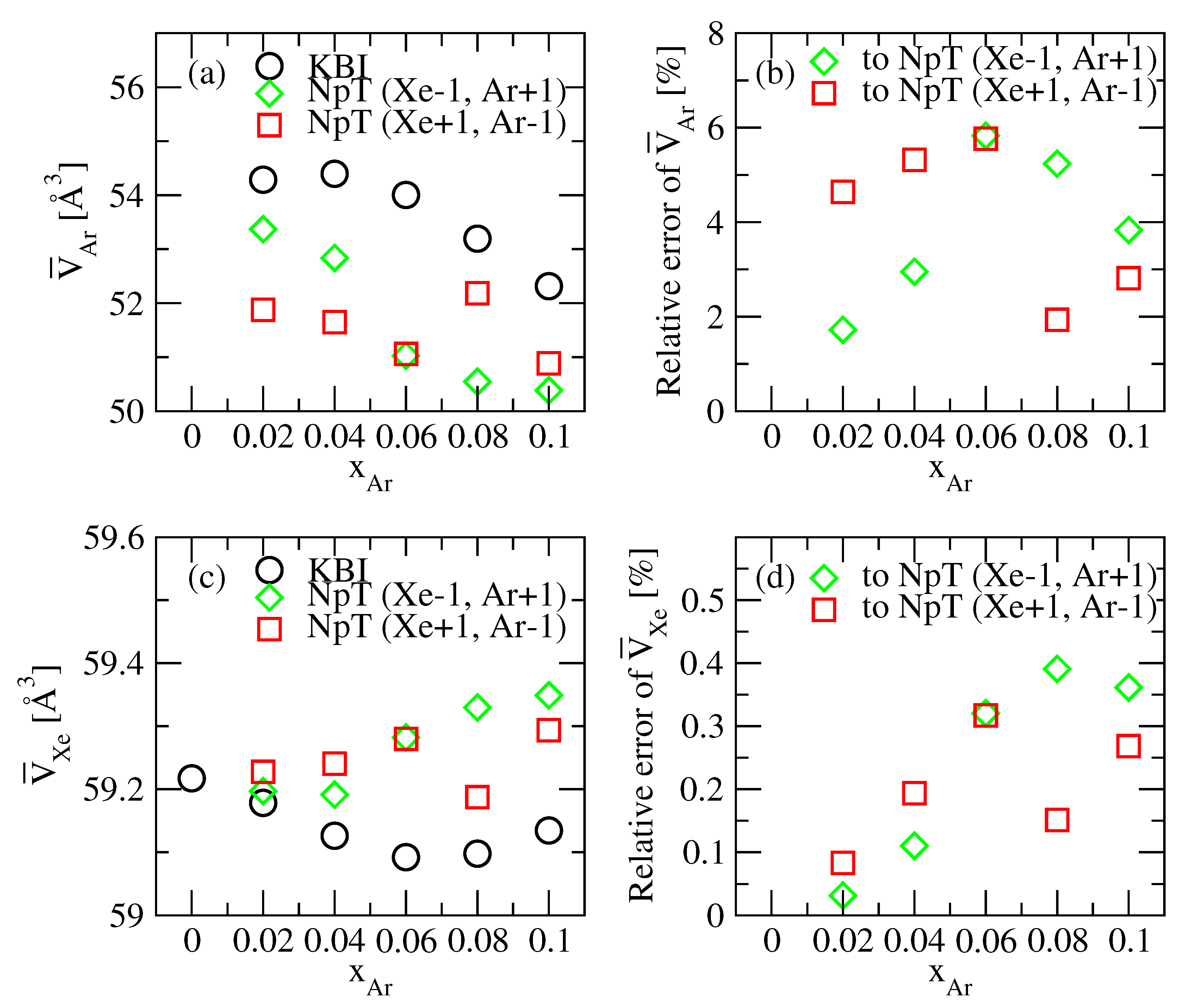
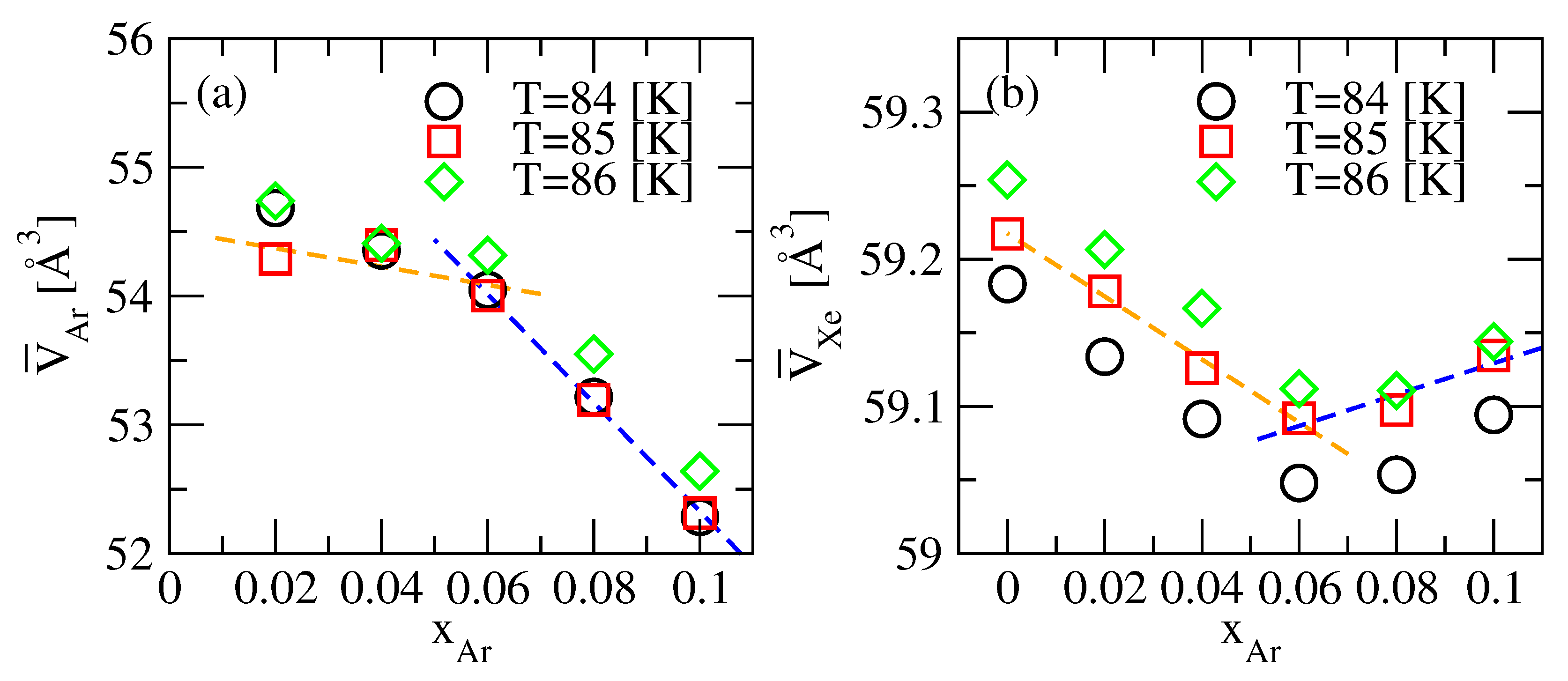
3.2. KBI and Partial Molar Volumes

Before computing the KBIs, the RDFs obtained from the NVT simulations were convoluted using Equation (12), and the Ganguly and van der Vegt’s correction, Equation (15), was applied. The result, for $T=85$ K and $x_{\mathrm{Ar}}=2$%, is shown in Figure 3a.

The convolution of the RDF smears out the long-range oscillations and makes the KBIs converge fast [13]. Although most structural information of the RDF seems to be lost after convolution, two interesting features remain. First, all ${\tilde{g}}_{\alpha \beta }\left(r\right)$ graphs show a dip at $r=0$, which reflects the excluded volume effect. Second, the RDF ${\tilde{g}}_{\mathrm{ArAr}}\left(r\right)$ (and only this) has a pronounced peak at $r\approx 5$ Å, which means that, around a given Ar atom, there is an increased probability to find other Ar atoms in close vicinity. In other words, Ar atoms tend to accumulate, which confirms the conclusion drawn above from the analysis of Figure 1 and Figure 2. From the convoluted and corrected RDFs, the KBIs ${\tilde{G}}_{\alpha \beta }^{\mathrm{vdV}}$ are calculated using the finite-volume KBI method Equation (7) and shown in Figure 3b. The Xe-Xe and the Xe-Ar KBIs are negative, as in the case of a monoatomic crystal, where the KBI goes to $-1/\rho$ for $L\to \infty$ and $T\to 0$ [13]. Interestingly, however, the Ar-Ar KBI has a large positive value, which signals a tendency of the solute (Ar) to accumulate [28].

We next analyse the partial molar volumes. Figure 4a shows ${\overline{V}}_{\mathrm{Ar}}$ and ${\overline{V}}_{\mathrm{Xe}}$ as a function of L, calculated from the KBIs using Equation (8). The values in the thermodynamic limit $(L\to \infty )$ were estimated by fitting the slope of the graph $L\times \overline{V}$ at large L; see Figure 4b. This fitting was performed for each temperature and concentration, and the obtained partial molar volumes are listed in Table 3. For $T=85$ K, the data are plotted in Figure 5a,c and compared with the partial molar volumes obtained from NpT simulation and Equation (21). From the latter, we obtained two values, depending on whether Ar was replaced by Xe or vice versa. The two values differ by up to 3% for Ar and 0.3% for Xe, which gives an error estimation for this method.

The difference between the partial molar volumes obtained with the KBI and NpT is at a maximum of 6% for Ar and 0.4% for Xe, and so, the KBI error is comparable to the NpT error; see Figure 5b,d. The fact that the error of the minority type (Ar) is much larger than that of the majority type (Xe) is expected because of poorer statistics for the minority type.

The partial molar volumes of Ar and Xe obtained from the KBIs are plotted in Figure 6. The dependence on Ar concentration $x_{\mathrm{Ar}}$ clearly changes at $x_{\mathrm{Ar}}\approx 0.06$. The slopes of the ${\overline{V}}_{\mathrm{Ar}}$ plot (Figure 6a) are −7.1 Å${}^3$ for $x_{\mathrm{Ar}}<6\%$ and −42.2 Å${}^3$ for $x_{\mathrm{Ar}}>6\%$, i.e., much larger at a higher Ar concentration. The corresponding slopes of the ${\overline{V}}_{\mathrm{Xe}}$ plot (Figure 6b) are −2.1 Å${}^3$ for $x_{\mathrm{Ar}}<6\%$ and 1.1 Å${}^3$ for $x_{\mathrm{Ar}}>6\%$. The variation of the partial molar volume of Xe is smaller than that of Ar and can be regarded as almost constant.

This rapid decrease in the partial molar volumes of Ar at higher concentrations may reflect an increase in the occurrence of Ar clusters. From the analysis of the RDFs, we found that the Ar atoms are bound to the Xe lattice sites for $x_{\mathrm{Ar}}<5\%$, so their partial molar volume is large and close to that of Xe. For $x_{\mathrm{Ar}}>5\%$, Ar clusters of three or more atoms start forming. In such clusters, the Ar-Ar distance can relax and approach the much smaller value of pure Ar. As a consequence, the partial molar volume of Ar decreases fast, as seen in Figure 6a. Note that the partial molar volume of Ar is smaller than that of Xe, even at the lowest Ar concentration because the Xe atoms relax a little around the Ar impurity (see Figure 1b).

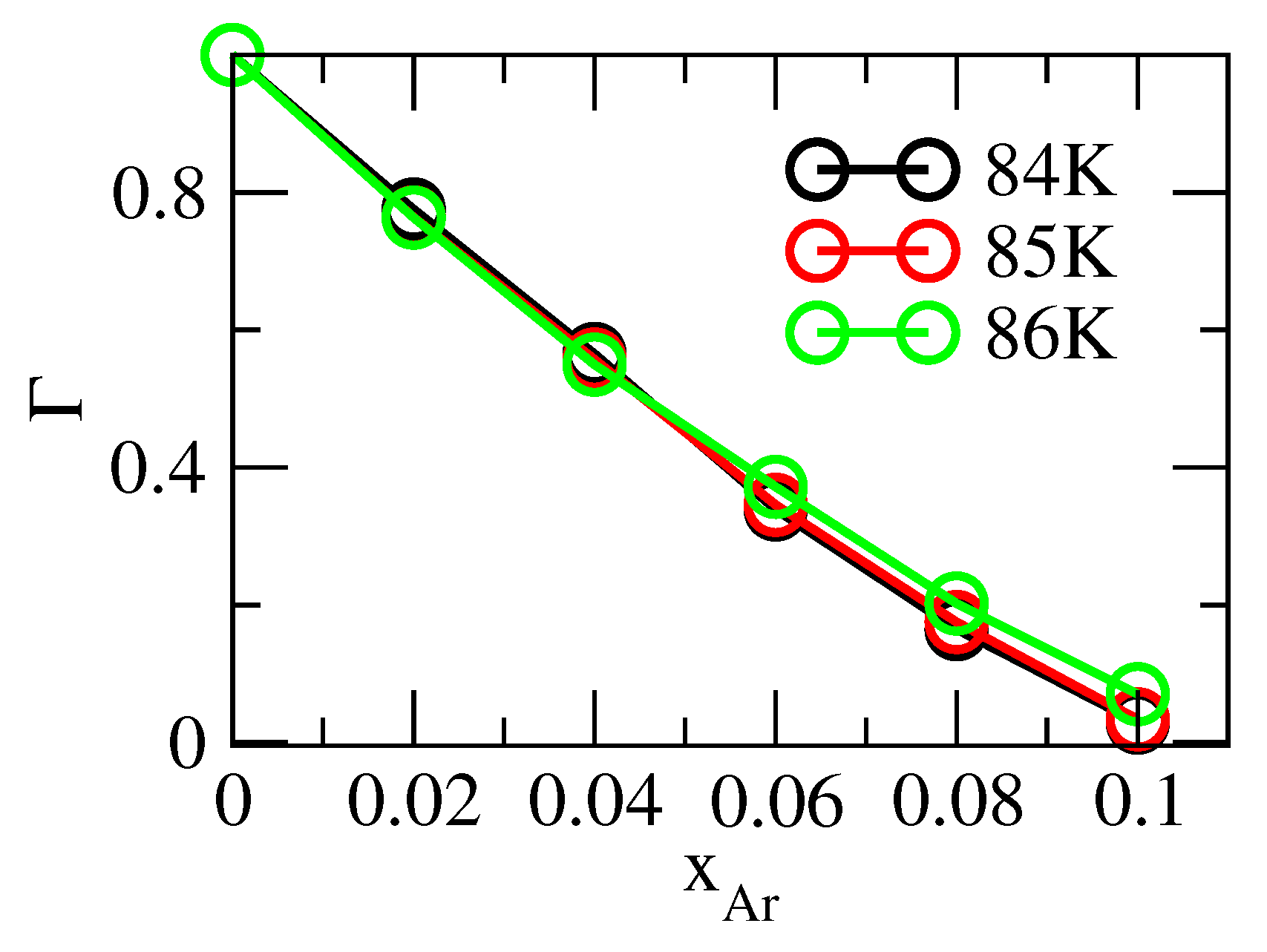
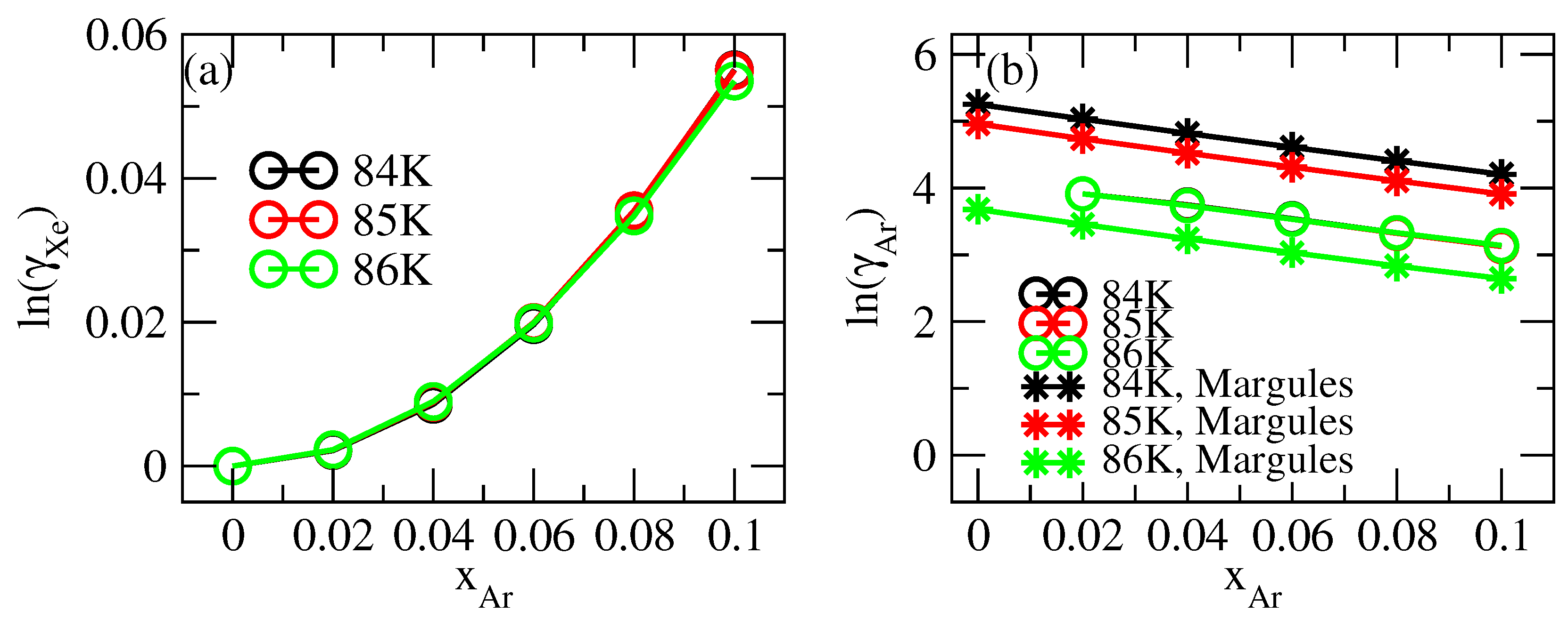
3.3. Thermodynamic Correction Factor and Chemical Potential

In the theory of liquids, the non-ideality of the solution mixture is often described by the thermodynamic correction factor $\Gamma$. This quantity gives access to the evolution of the chemical potential with the molar fraction. For example, when calculating Fick’s diffusion coefficient from MD simulation, it accounts for the thermodynamic contribution to the transport property. For an ideal mixture (in the sense that ideal mixing rules apply), $\Gamma$ equals 1, but it has a different value otherwise. The $\Gamma$ values calculated from Equation (10) are plotted as a function of the Ar concentration in Figure 7 for the three different temperatures.

As expected, $\Gamma \to 1$ for $x_{\mathrm{Ar}}\to 0$. For $x_{\mathrm{Ar}}>0$, $\Gamma$ decreases linearly until $x_{\mathrm{Ar}}$ = 0.05, where the curve starts to bend, but it keeps decreasing and goes to zero for $x\approx 0.1$. It is well known that when $\Gamma \approx 0$, the values of $x_{\mathrm{Ar}}$ change drastically for a small change in chemical potential, which is a clear sign of a transition from one phase, here the solid solution for $x_{\mathrm{Ar}}<0.1$, to another phase for $x_{\mathrm{Ar}}>0.1$. Despite the uncertainty of the data, it is evident from the plot that this transition point (the $x_{\mathrm{Ar}}$ value where $\Gamma =0$) decreases with temperature.

The knowledge of $\Gamma$ for different values of $x_{\mathrm{Ar}}$ gives the possibility to compute the variation of the chemical potential of Ar or Xe from a reference point. This is performed by integrating $\Gamma$ with $lnx$. For Xe, the reference point is the pure xenon solid phase, while for Ar, we used the composition $x_{\mathrm{Ar}}$ = 0.02. The results are presented in Figure 8. It is seen that the chemical potentials tend to constant values above $x_{\mathrm{Ar}}$ = 0.1, which is a clear sign of a phase transition. This is in agreement with the analysis on the partial molar volumes.

The evolution of the chemical potential with composition can also be analysed with thermodynamic models. From the chemical potential, the activities $a=\gamma x$, and the activity coefficients $\gamma$, of the two species are calculated and presented in Figure 9 and Figure 10, respectively. For Xe, the activities deviate slightly from 1, while for Ar, they vary linearly with molar fraction for small values of $x_{\mathrm{Ar}}$ before showing a plateau. This linear evolution is equivalent to Henry’s regime for the dissolution of a gas in a liquid.

In Figure 10b, it is seen that $ln{\gamma }_{\mathrm{Xe}}$ has a cubic behaviour with Ar concentration; this trend is characteristic of a mixture that obeys the three-suffix Margules equations:

$$\begin{array}{ccc}\hfill ln{\gamma }_{\mathrm{Xe}}& =& b{x}_{\mathrm{Ar}}^2+c{x}_{\mathrm{Ar}}^3,\hfill \end{array}$$

(22)

$$\begin{array}{ccc}\hfill ln{\gamma }_{\mathrm{Ar}}& =& \frac{2b+3c}{2}{x}_{\mathrm{Xe}}^2-c{x}_{\mathrm{Xe}}^3.\hfill \end{array}$$

(23)

The parameters b and c were obtained by fitting Equation (22) to the data in Figure 10a and are given in

Table 4. Margules parameter values.

Temperature	84 (K)	85 (K)	86 (K)
b	5.54457	5.63663	5.76786
c	−0.58653	−1.35139	−4.17325

. The values of $ln{\gamma }_{\mathrm{Ar}}$ as obtained from the Margules Equation (23) are plotted in Figure 10b and compared with the data derived from the thermodynamic factor $\Gamma$. In the range of the presented molar fraction ($x_{\mathrm{Ar}}<0.1$), $ln{\gamma }_{\mathrm{Ar}}$ decreases linearly with $x_{\mathrm{Ar}}$, and the slope is the same for all data sets. In the Margules data (stars), the reference state is $x_{\mathrm{Ar}}$ = 0, while it is $x_{\mathrm{Ar}}$ = 0.02 for the data from the thermodynamic factor (circles); this explains the vertical offsets. In other words, by virtue of the Margules equations, we can estimate ${\gamma }_{\mathrm{Ar}}$ for $x_{\mathrm{Ar}}\to 0$ from the known (ideal) behaviour of the solvent in the dilute limit, namely $ln{\gamma }_{\mathrm{Xe}}\to 0$. As a result (see Figure 10b, stars), we find that ${\gamma }_{\mathrm{Ar}}$ has a temperature dependence.

Within the Margules model, the activity coefficients are fully determined by the knowledge of the parameters b, c. This allows us to extrapolate the activity from the narrow interval $x_{\mathrm{Ar}}$, for which simulation data exist, to the whole composition range $0<x_{\mathrm{Ar}}<1$; see Figure 11. All the curves show two extrema, one at $x_{\mathrm{Ar}}\approx 0.1$, close to the previously discussed stability limit of the Xe-rich solid phase, and a second extremum at $x_{\mathrm{Ar}}$ between 0.7 and 0.9, depending on the temperature. For compositions between these two extrema, the system is unstable and favours phase separation. Some authors reported this kind of behaviour, using thermodynamic models and experiments [16,29,30]. It is important to note that the quality of the extrapolation shown in Figure 11, depends both on the accuracy of the simulation results and on the model used for the activity coefficients (Margules in this case). Other models such as UNIQUAC or NRTL could predict a somewhat different unstable zone.

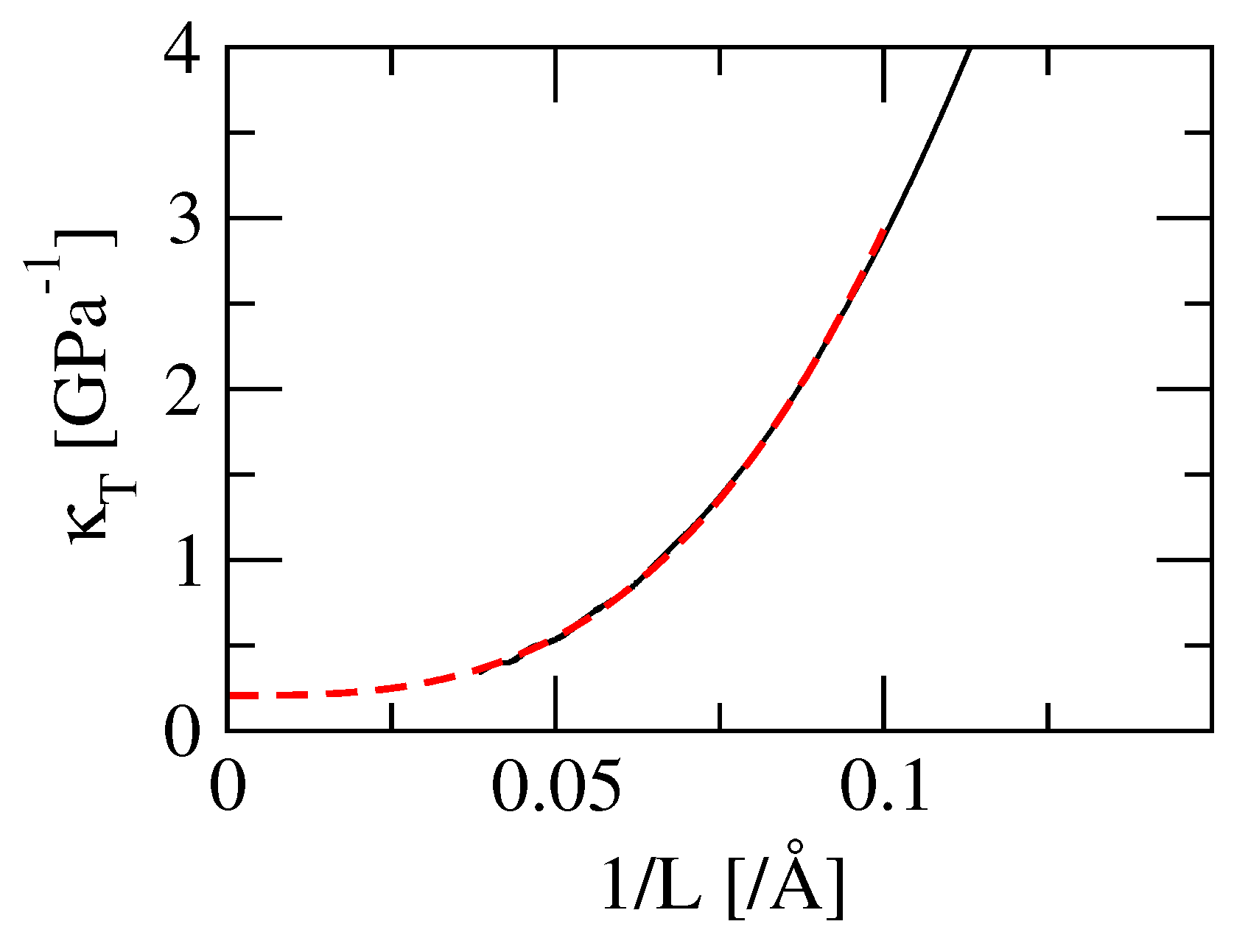
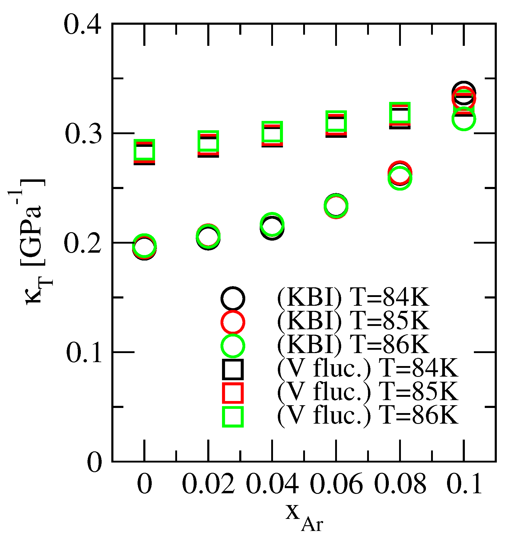
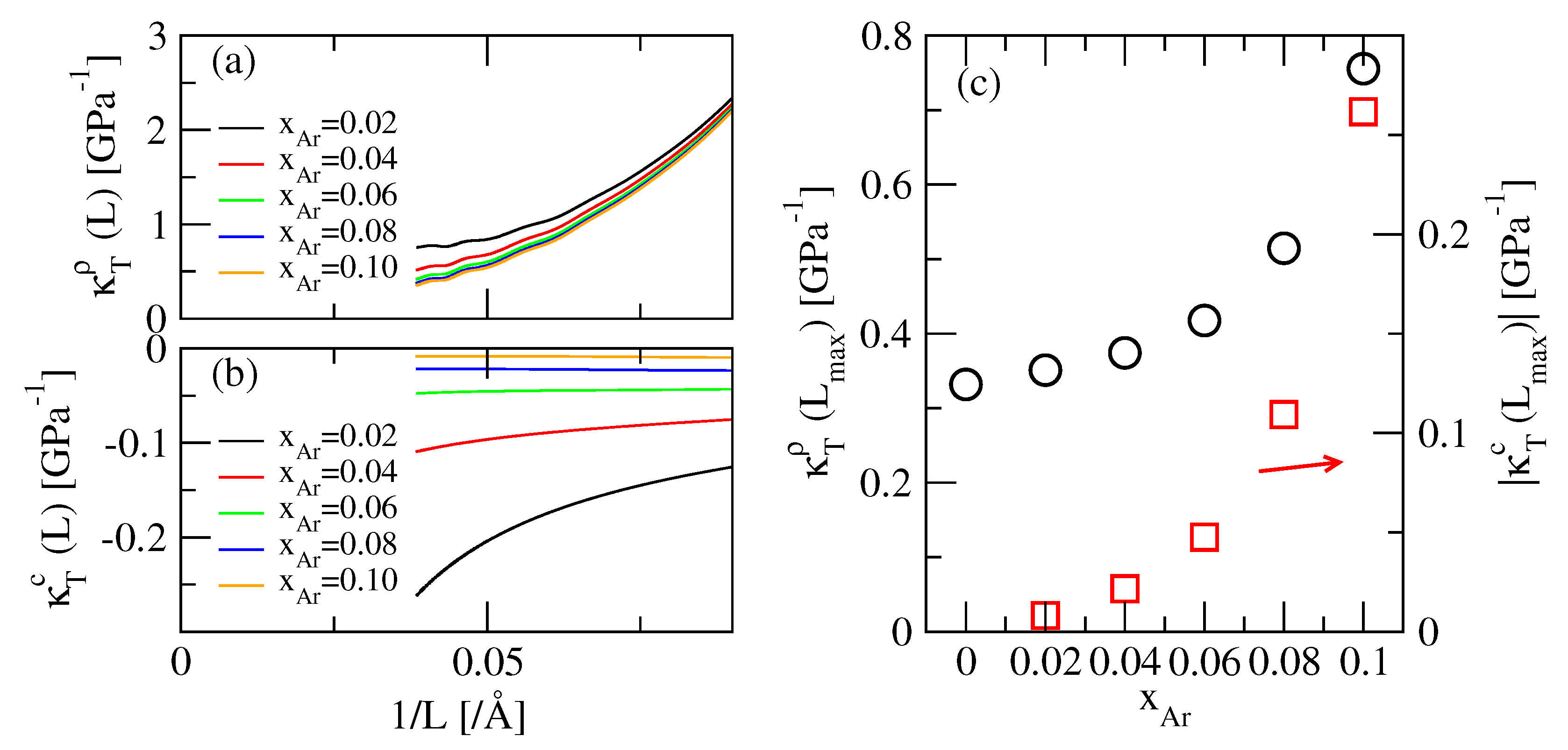
3.4. Isothermal Compressibility

The isothermal compressibility as a function of L is shown in Figure 12 for an Ar-Xe mixture at $T=85$ K and $x_{\mathrm{Ar}}=2$%, using the same KBIs (Figure 3b) from which the partial molar volumes were obtained.

The convergence value of this isothermal compressibility can be obtained by applying cubic fitting to this function (Figure 12). The convergence values were calculated by the same method at each temperature and Ar concentration. They are listed in Table 2.

Figure 13 shows the isothermal compressibility ${\kappa }_T^{\mathrm{KBI}}$ from the KBI and ${\kappa }_T^{\mathrm{NpT}}$ from the volume fluctuations as a function of Ar concentration. In the temperature and concentration range treated in this study, the isothermal compressibility varies more strongly with Ar concentration than with temperature, which is consistent between the KBI and volume fluctuation results. However, while the variation with $x_{\mathrm{Ar}}$ is linear for the volume fluctuation values, a non-linear dependence is seen for the KBI-derived values. For $x\le 0.04$, the compressibility values from the KBI are smaller, by about 30%, than those obtained from volume fluctuations, which are known to be much more accurate (by comparison with $T\to 0$ and $x_{\mathrm{Ar}}=0$). A similar error of the KBI-derived compressibility was obtained for solid Ar [13]. For $x_{\mathrm{Ar}}>0.05$, the KBI values rise quickly and approach those from the volume fluctuations. However, this decrease of the error is fortuitous, because for $x>0.1$, the compressibility becomes much too large, i.e., the error increases with the opposite sign, as we checked. This sharp rise of the KBI-derived compressibility for $x_{\mathrm{Ar}}>0.05$ is likely due to the appearance of Ar clusters, which we believe are precursors of the Ar-rich liquid phase; see Section 3.2. Clustering induces a strong structural inhomogeneity, and so, KBI theory, which assumes the homogeneity of the system, might not be fully valid for $x_{\mathrm{Ar}}>0.05$.

Finally, we discuss the relative contribution of density and concentration fluctuations to the compressibility. In a two-component system with species $\alpha$, $\beta$, the isothermal compressibility can be expressed as ${\kappa }_T={\kappa }_T^{\rho }+{\kappa }_T^c$, i.e., the sum of a density fluctuation term ${\kappa }_T^{\rho }$ and a composition fluctuation term ${\kappa }_T^c$, given by [31]

$$\begin{array}{cc}\hfill {\kappa }_T^{\rho }& =\frac{〈{(\Delta N)}^2〉}{\langle N\rangle \rho kT}\hfill \end{array}$$

(24)

$$\begin{array}{cc}\hfill & =\frac{x_{\alpha }{\rho }_{\alpha }{G}_{\alpha \alpha }+x_{\beta }{\rho }_{\beta }{G}_{\beta \beta }+2x_{\alpha }{x}_{\beta }\rho G_{\alpha \beta }+1}{\rho kT},\hfill \end{array}$$

(25)

$$\begin{array}{cc}\hfill {\kappa }_T^c& =-\frac{{({\overline{V}}_{\alpha }-{\overline{V}}_{\beta })}^2\rho N〈{(\Delta x)}^2〉}{kT}\hfill \end{array}$$

(26)

$$\begin{array}{cc}\hfill & =-\frac{{\{{\rho }_{\alpha }\left(G_{\alpha \alpha }-G_{\alpha \beta }\right)-{\rho }_{\beta }\left(G_{\beta \beta }-G_{\alpha \beta }\right)\}}^2{x}_{\alpha }{x}_{\beta }}{kT\{{\rho }_{\alpha }+{\rho }_{\beta }+{\rho }_{\alpha }{\rho }_{\beta }\left(G_{\alpha \alpha }^{\infty }+G_{\beta \beta }^{\infty }-2G_{\alpha \beta }^{\infty }\right)\})}.\hfill \end{array}$$

(27)

Here, N is the number of all particles in the system, $\Delta N=N-〈N〉$, $\rho =\langle N/V\rangle$, and $\Delta x$ is defined by $\Delta x=[x_{\beta }\Delta N_{\alpha }-x_{\alpha }\Delta N_{\beta }]/N$.

The two terms are plotted in Figure 14a,b as a function of L for $T=85$ K. It is seen that the concentration term ${\kappa }_T^c\left(L\right)$ does not converge for $L\to \infty$ when $x_{\mathrm{Ar}}>0.06$, and thus, the KBI-derived isothermal compressibility values in Figure 13 are not accurate for these Ar concentrations. However, from the comparison of the values at the endpoints of these functions $L_{\max }$ (Figure 14c), it is clear that the absolute values of both the density and concentration fluctuation components increase rapidly when $x_{\mathrm{Ar}}$ is higher than 5%, which is understood to be due to the onset of the separation of the solid and liquid phases by the formation of Ar clusters.

4. Conclusions

In this study, we demonstrated that KBI solution theory can be applied not only to liquids, but also to solid solutions, and we discussed the structural and thermodynamic information that can be obtained from the KBIs. We applied the theory to Xe-rich Ar-Xe mixtures with radial distribution functions obtained from MC simulations and calculated the KBIs using the finite-volume KBI method. The partial molar volumes obtained from the KBI agree well with the values with a standard method. From the concentration dependence of the KBI and the partial molar volume, it was found that for an Ar concentration $x_{\mathrm{Ar}}<5$%, the Xe crystal structure relaxes around the mostly isolated Ar impurities, while for $x>5$%, a fast variation of the KBI and partial molar volumes is observed due to Ar cluster formation. From the KBIs, the thermodynamic correction factor is obtained and the chemical potentials of Ar and Xe are estimated by integration over the molar fraction. By fitting the data to the Margules equations, the activity coefficients for the whole composition range were obtained, which shows that the Xe-rich solid phase is unstable for $x>0.1$, in agreement with the literature. We conclude that the computation of KBIs in solid solutions provides valuable insights into the structure of the mixture and its thermodynamic phase stability.

References

1. Kirkwood, J.G.; Buff, F.P. The Statistical Mechanical Theory of Solutions. I. J. Chem. Phys. 1951, 19, 774–777. [Google Scholar] [CrossRef]
2. Ben-Naim, A. Inversion of the Kirkwood–Buff theory of solutions: Application to the water–ethanol system. J. Chem. Phys. 1977, 67, 4884–4890. [Google Scholar] [CrossRef]
3. Liu, X.; Martin-Calvo, A.; McGarrity, E.; Schnell, S.K.; Calero, S.; Simon, J.M.; Bedeaux, D.; Kjelstrup, S.; Bardow, A.; Vlugt, T.J.H. Fick diffusion coefficients in ternary liquid systems from equilibrium molecular dynamics simulations. Ind. Eng. Chem. Res. 2012, 51, 10247. [Google Scholar] [CrossRef]
4. Fingerhut, R.; Herres, G.; Vrabec, J. Thermodynamic factor of quaternary mixtures from Kirkwood–Buff integration. Mol. Phys. 2020, 118, e1643046. [Google Scholar] [CrossRef]
5. Perera, A.; Sokolić, F. Modeling nonionic aqueous solutions: The acetone-water mixture. J. Chem. Phys. 2004, 121, 11272–11282. [Google Scholar] [CrossRef]
6. Ganguly, P.; van der Vegt, N.F.A. Convergence of Sampling Kirkwood–Buff Integrals of Aqueous Solutions with Molecular Dynamics Simulations. J. Chem. Theory Comput. 2013, 9, 1347–1355. [Google Scholar] [CrossRef]
7. Collell, J.; Galliero, G. Determination of the thermodynamic correction factor of fluids confined in nano-metric slit pores from molecular simulation. J. Chem. Phys. 2014, 140, 194702. [Google Scholar] [CrossRef]
8. Fingerhut, R.; Vrabec, J. Kirkwood–Buff integration: A promising route to entropic properties? Fluid Phase Equilibria 2019, 485, 270–281. [Google Scholar] [CrossRef] [Green Version]
9. Kobayashi, T.; Reid, J.E.S.J.; Shimizu, S.; Fyta, M.; Smiatek, J. The properties of residual water molecules in ionic liquids: A comparison between direct and inverse Kirkwood–Buff approaches. Phys. Chem. Chem. Phys. 2017, 19, 18924–18937. [Google Scholar] [CrossRef] [Green Version]
10. Dawass, N.; Krüger, P.; Schnell, S.; Simon, J.M.; Vlugt, T.J.H. Kirkwood–Buff integrals from molecular simulation. Fluid Phase Equilibria 2019, 486, 21–36. [Google Scholar] [CrossRef]
11. Proffen, T.; Billinge, S.J.L.; Egami, T.; Louca, D. Structural analysis of complex materials using the atomic pair distribution function—A practical guide. Z. Kristallogr. Cryst. Mater. 2003, 218, 132–143. [Google Scholar] [CrossRef]
12. Billinge, S.J.L.; Levin, I. The Problem with Determining Atomic Structure at the Nanoscale. Science 2007, 316, 561–565. [Google Scholar] [CrossRef] [PubMed] [Green Version]
13. Miyaji, M.; Radola, B.; Simon, J.M.; Krüger, P. Extension of Kirkwood–Buff theory to solids and its application to the compressibility of fcc argon. J. Chem. Phys. 2021, 154, 164506. [Google Scholar] [CrossRef] [PubMed]
14. Krüger, P. Validity of the compressibility equation and Kirkwood–Buff theory for crystalline matter. Phys. Rev. E 2021, 103, L061301. [Google Scholar] [CrossRef] [PubMed]
15. Krüger, P.; Schnell, S.K.; Bedeaux, D.; Kjelstrup, S.; Vlugt, T.J.H.; Simon, J.M. Kirkwood–Buff Integrals for Finite Volumes. J. Phys. Chem. Lett. 2013, 4, 235–238. [Google Scholar] [CrossRef] [PubMed]
16. Campestrini, M.; Stringari, P.; Arpentinier, P. Solid–liquid equilibrium prediction for binary mixtures of Ar, O2, N2, Kr, Xe, and CH4 using the LJ-SLV-EoS. Fluid Phase Equilibria 2014, 379, 139–147. [Google Scholar] [CrossRef] [Green Version]
17. Krüger, P. Ensemble averaged Madelung energies of finite-volumes and surfaces. Phys. Rev. B 2020, 101, 205423. [Google Scholar] [CrossRef]
18. Dawass, N.; Krüger, P.; Schnell, S.K.; Bedeaux, D.; Kjelstrup, S.; Simon, J.M.; Vlugt, T.J.H. Finite-size effects of Kirkwood–Buff integrals from molecular simulations. Mol. Simul. 2018, 44, 599–612. [Google Scholar] [CrossRef]
19. Krüger, P.; Vlugt, T.J.H. Size and shape dependence of finite-volume Kirkwood–Buff integrals. Phys. Rev. E 2018, 97, 051301. [Google Scholar] [CrossRef] [Green Version]
20. Dawass, N.; Krüger, P.; Simon, J.M.; Vlugt, T.J.H. Kirkwood–Buff integrals of finite systems: Shape effects. Mol. Phys. 2018, 116, 1573–1580. [Google Scholar] [CrossRef] [Green Version]
21. Santos, A. Finite-size estimates of Kirkwood–Buff and similar integrals. Phys. Rev. E 2018, 98, 063302. [Google Scholar] [CrossRef] [Green Version]
22. Cortes-Huerto, R.; Kremer, K.; Potestio, R. Communication: Kirkwood–Buff integrals in the thermodynamic limit from small-sized molecular dynamics simulations. J. Chem. Phys. 2016, 145, 141103. [Google Scholar] [CrossRef] [PubMed] [Green Version]
23. Mick, J.R.; Soroush Barhaghi, M.; Jackman, B.; Rushaidat, K.; Schwiebert, L.; Potoff, J.J. Optimized Mie potentials for phase equilibria: Application to noble gases and their mixtures with n-alkanes. J. Chem. Phys. 2015, 143, 114504. [Google Scholar] [CrossRef] [PubMed]
24. Lorentz, H.A. Ueber die Anwendung des Satzes vom Virial in der kinetischen Theorie der Gase. Ann. Physik 1881, 248, 127–136. [Google Scholar] [CrossRef] [Green Version]
25. Berthelot, D. Sur le mélange des gaz. Compt. Rendus 1898, 126, 1703–1706. [Google Scholar]
26. Purton, J.; Crabtree, J.; Parker, S. DL_MONTE: A general purpose program for parallel Monte Carlo simulation. Mol. Simul. 2013, 39, 1240–1252. [Google Scholar] [CrossRef]
27. Brukhno, A.V.; Grant, J.; Underwood, T.L.; Stratford, K.; Parker, S.C.; Purton, J.A.; Wilding, N.B. DL_MONTE: A multipurpose code for Monte Carlo simulation. Mol. Simul. 2019, 47, 131–151. [Google Scholar] [CrossRef] [Green Version]
28. Primorac, T.; Pozar, M.; Sokolić, F.; Zoranić, L. The influence of binary mixtures’ structuring on the calculation of Kirkwood–Buff integrals: A molecular dynamics study. J. Mol. Liq. 2021, 324, 114773. [Google Scholar] [CrossRef]
29. Manzhelii, V.G.; Prokhvatilov, A.I.; Minchina, I.Y.; Yantsevich, L.D. Handbook of Binary Solutions of Cryocrystals; Begell House: New York, NY, USA, 1996. [Google Scholar]
30. Yantsevich, L.D.L.; Prokhvatilov, A.I.; Barylnik, A.S. Phase diagrams of Ar-Xe, Kr-Xe and Kr-CO binary alloys. Fiz. Nizk. Temp. 1996, 22, 218–221. [Google Scholar]
31. Bhatia, A.B.; Thornton, D.E. Structural Aspects of the Electrical Resistivity of Binary Alloys. Phys. Rev. B 1970, 2, 3004–3012. [Google Scholar] [CrossRef]
Figure 1. RDFs and information obtained from RDFs. (a) RDFs at T = 85 K and x Ar = 0.02 . (b) RDFs enlarged around nearest neighbour distances at T = 85 K and x Ar = 0.02 (broken lines) or x Ar = 0.10 (solid lines). (c) Nearest neighbour distances ( R 1 ) normalised by their values at x Ar = 0.02 . (d) The mean number of Ar nearest neighbours around an Ar atom (Ar-Ar) or a Xe atom (Xe-Ar).
Physchem 02 00014 g001
Figure 2. Snapshots of (111) planes of Ar-Xe mixtures at T = 84 K and (a) x Ar = 0.02 and (b) x Ar = 0.10 .
Physchem 02 00014 g002
Figure 3. (a) RDFs convoluted by Equation (12) and corrected by Equation (15) at T = 85 K and x Ar = 0.02 . (b) KBIs calculated by Equation (7) using (a).
Physchem 02 00014 g003
Figure 4. (a) Partial molar volumes V ¯ Ar (black) and V ¯ Xe (red) from the KBI as a function of L, at T = 85 K and x Ar = 0.02 . (b) Plot of L × V ¯ Ar and L × V ¯ Xe and linear fits (green and blue lines).
Physchem 02 00014 g004
Figure 5. Partial molar volumes, (a) V ¯ Ar and (c) V ¯ Xe , at T = 85 K, from KBI (black), and NpT simulations with particle numbers ( N Xe −1, N Ar +1) (green) or ( N Xe +1, N Ar −1) (red). (b,d) show the relative errors of V ¯ Ar and V ¯ Xe from the KBI, with respect to the values obtained from NpT.
Physchem 02 00014 g005
Figure 6. Partial molar volumes from KBIs as a function of Ar concentration x Ar for different temperatures. V ¯ Ar in (a) and V ¯ Xe in (b). Broken lines are linear fits in the x Ar range 0.00–0.06 (orange) and 0.06–0.10 (blue).
Physchem 02 00014 g006
Figure 7. Thermodynamic correction factor as a function of Ar concentration.
Physchem 02 00014 g007
Figure 8. Evolution of the chemical potential of (a) Ar and (b) Xe as a function of the Ar concentration. Note that the reference point is x Ar = 0 for Xe, but it is x Ar = 0.02 for Ar.
Physchem 02 00014 g008
Figure 9. Activity of Ar and Xe as a function of the Ar concentration. Note that the reference point is x Ar = 0 for Xe, but it is x Ar = 0.02 for Ar.
Physchem 02 00014 g009
Figure 10. Evolution of ln γ with x Ar for (a) Xe and (b) Ar. Values obtained from simulation data via Γ (circles) or from a fit to the Margules equations (stars).
Physchem 02 00014 g010
Figure 11. Activity of Ar and Xe as a function of the Ar concentration calculated with the Margules equations.
Physchem 02 00014 g011
Figure 12. Isothermal compressibility (black) from KBIs at T = 85 K and x Ar = 0.02 as a function of L and cubic fit (red).
Physchem 02 00014 g012
Figure 13. Isothermal compressibility from KBIs (circle) and from volume fluctuations (square).
Physchem 02 00014 g013
Figure 14. The two terms contributing to the isothermal compressibility κ T = κ T ρ + κ T c , calculated for T = 85 K as a function of inverse system size 1 / L . (a) Density fluctuation term κ T ρ ( L ) (Equation (25)). (b) Concentration fluctuation term κ T c ( L ) (Equation (27)). (c) The absolute values of the endpoints (i.e., at maximum L).
Physchem 02 00014 g014