Benthic Fauna Assessment along the Navigation Channel from the Mouth of the Casamance Estuary to Ziguinchor City

Abstract

This study aimed at studying the benthic fauna of the Casamance estuary (Senegal) through the analysis of its composition at 13 stations located along the channel from the estuary mouth to Ziguinchor port (estuary upstream), which may provide indications of the potential environmental impact of the navigation channel dredged on the estuary. Sixty taxa distributed in twelve phyla were identified, of which the most abundant were bivalve mollusks, annelids, and nematodes. The species abundance and species richness varied from five (estuary mouth) to thirty species (upstream). Correspondence factorial analysis (CFA) and factor analysis for mixed data (FAMD) showed, respectively, that 34% (Dim 1 = 15.6% and Dim 2 = 18.4%) and 35.5% (Dim 1 = 20.8% and Dim 2 = 14.7%) of total inertia was explained by the first two axes and a significant correlation between the dominant species distribution, sediment type, and depth of the sampled station. Overall, Spearman’s rank correlation indicated a significant negative correlation of the species abundance and species richness with distance from the estuary mouth. From these results, it appears that sediment type, depth of the sampled stations, salinity, and the mangrove forests are key factors that influence the distribution and abundance of benthic fauna in the Casamance estuary. The monitoring plans for the preservation of the health and biological diversity of this ecosystem, especially benthic fauna biodiversity, should take into consideration the seasonal variations of rainfalls and related changes in terms of physicochemical factors. This should include evaluating the long-term responses of benthic organisms to dredging activities, boat traffic, and especially physical habitat modifications, changes in migration ways, and pollution pressure.

1. Introduction

Estuarine ecosystems are important natural environments characterized by diverse habitat mosaics and large organic matter resources [1,2,3,4]. Thus, they constitute optimal ecological niches and refuges for aquatic organisms, including benthic organisms [3,5,6]. Estuaries are also of economic and social importance, essentially due to the presence of abundant fishery resources and to their recreational and commercial transport benefits. Despite their socio-economic importance, these areas often suffer the adverse effects of industrialization and overdevelopment [7]. Estuaries are subject to the construction of diverse infrastructures, such as port construction, navigation channels, and harbors, which can degrade or destroy these habitats and therefore negatively impact the living organisms that inhabit them [8]. Road and port construction in estuarine areas releases large amounts of suspended sediments that may alter the physical conditions of the ecosystem [9]. The presence of navigation channels and ports can also cause considerable anthropogenic disturbances that may lead to the degradation of habitats [10]. The presence of navigation channels can be associated with other environmental issues including emission of pollutants, sediment dredging, industrial installations and associated negative impacts, jetty construction, and wastewater discharges [10]. The use of maritime roads and their maintenance can cause environmental contamination of the surrounding areas by different classes of chemicals, such as heavy metals, salt, organic molecules and nutrients [10].

Channel dredging on aquatic areas does not only provoke physical changes in habitats, but it may also cause modification of animal behavior and/or the accidental introduction of invasive species, which may disrupt native communities [11]. This may result in the recruitment of opportunistic species that are less affected by environmental changes and that may, over time, replace equilibrium species more adapted to stable environments [11,12]. The presence of roads may negatively affect animal behavior through habitat shifts and the alteration of movement patterns, reproductive success, escape response, and physiological state [13,14,15]. Road construction may directly kill aquatic organisms or cause stress that leads to death and therefore impair aquatic productivity [10]. The chemicals and marine sediments contaminated by weathered and biodegraded components resulting from maritime road construction and its use may represent a persistent and ongoing threat for benthic organisms [16].

The assessment of environmental impacts (habitat and benthic faunal characterization) prior to the implementation of infrastructures such as navigation channels is crucial to identify zones of high biological diversity or areas inhabited by endangered species that would be damaged by construction and associated anthropogenic activities. Environmental assessment studies can be used to evaluate the degree of damage that would be caused by maritime channel dredging, boat traffic, and eventual impacts on ecosystems and living organisms [17]. Such studies can help to develop appropriate and sustainable management plans for biodiversity restoration when pollution accidents occur on road channels or surrounding areas [18,19,20,21]. Therefore, initial habitat and faunal characterization is essential prior to the construction of maritime road channels.

To facilitate the maritime transport from the port of Ziguinchor (Senegal), a main navigation channel was dredged by the Senegalese public authorities through a project funded by the Royal Haskoning DHV firm [22]. The channel that was constructed along the Casamance estuary has a depth that generally decreases from downstream to upstream (from 12 to 7 m in depth, respectively). This rise of the sediment bottom of the tidal wave favors the silting-up of the channel, with probable impacts on animal and plant biodiversity and on the navigability of the estuary. Understanding the impacts of such disturbances on the health of the ecosystem and on the diversity of species remains a challenge. The purpose of the current study was to assess the biodiversity of benthic fauna at the chosen stations through the analysis of species composition, distribution, and abundance. Such analyses can provide information on the initial state and the quality of the ecosystem. Indeed, some benthic species are biological, ecological indicators of the aquatic environments they inhabit and may therefore provide indications of the ecosystem health.

2. Material and Methods

2.1. Study Area

The Casamance is a natural region located in the south of Senegal between the republics of Gambia and Guinea. The region has a coastline of around 100 km and is bordered by the Casamance estuary, which originates east of Kolda in Fouladou [23]. The Casamance River is of great economic importance and is host to various human activities, such as rice growing, fishing and trade. The river, which is approximately 350 km long (including 260 km of permanent course) drains a catchment area of 14,000 km² [24]. It is fed by numerous tributaries and several bolons (saline rivers originating in the mangroves) towards the estuary mouth and its water supplies are estimated at 60 million m³ per year. These water resources allow the development of agriculture, help meet the water-related needs of people and livestock, and maintain biodiversity [25]. The generally favorable climatic conditions and the relative density of the hydrographic network ensure a high level of plant and animal diversity in the Casamance region. The hydroclimate of the estuary essentially depends on the water balance, which is negative due to the weakness of the slope and the ascent of seawater inland. The Casamance River has thus become, since the drought years of the 1960s, an inverse estuary with salinity that increases with the distance from the mouth [26,27]. This inverse salinity gradient and marine invasion up to 200 km results from limited freshwater inputs, a weak slope, and intense water evaporation [28].

2.2. Sampling Stations and Equipment

Thirteen sampling stations (1 to 13) located from the estuary mouth to Ziguinchor city (located further upstream) were subjected to benthic sample collection (Figure 1). The materialization (geo-referenced coordinates) of the stations was defined by The Royal Haskoning DHV (RHDHV). The stations were positioned on both the main channel and river banks to cover different benthic communities present in the estuary. The replicate samples were collected during sampling campaigns at the Casamance River from 7–17 March 2014. Sample collection was performed using a 225 cm² Ekman-type sediment bucket closed by a messenger and, if necessary, weighted to prevent drifting with strong currents. The number of replicates for each sampling station is indicated in

Table 1. Description of sampling sites and replicates used for benthic fauna collection.

Station	Location	Location Codes	Depth (m)	Type of Sediment	Codes of Sediment Type	Number of Replicates for Sampling of Benthic Fauna
S01	Dredge footprint (Zone C)	ZNC	2	mud	MD	3
S02	Upstream port	UP	4	mud	MD	3
S03	Refueling pontoon	RP	4	mud	MD	3
S04	Approach berth	AB	10	shell debris mixed with sandy mud	SD1	3
S05	River bed upstream	RB1	7	coarse particles in muddy sand	CP	5
S06	Boudody pontoon		4	silty mud		no benthic fauna at this location
S07	River bed downstream	RB2	9	sandy mud	SM1	3
S08	Eastern channel—river influence	EC	1	solid dark grey slightly sandy mud	SD2	4
S09	North bank opposite Ile Carabanes	NO	8	sandy mud mixed with shell debris	SM2	3
S10	West dredge footprint (Zone B)	ZNB	2	muddy sand mixed with great number of shell debris	MG	4
S11	East dredge footprint (Zone B)	ZNB	4	muddy sand mixed with shell debris	MS	5
S12	River bed toward Pt St Georges	RB3	5	grey mud	GM1	3
S13	Navigation channel o warddiogue	NC	4	grey muddy sand	GM2	3

.

2.3. Collection of Samples

Samples were collected with a minimum of 3 replicates per station, depending on the filling rate of the bucket, but some additional replicates were made in some sampling locations (Stations 5, 8, 10, and 11). Thus, a total of 42 replicates were made at the 13 sampling stations (Table 1). Each sample was screened with 2 mm and 0.85 mm diameter meshes. Refusals were then fixed in alcohol (ethanol 70%) and put in jars and/or plastic bags. The collected samples were then stored at room temperature until processing.

2.4. Description of Sediments and Sample Sorting in the Laboratory

In the laboratory, samples were sieved to determine the nature of the sediments and to identify species through visual observation. RoseBengal (protein dye) at 1 g/L was added to each sample until the coloration of the individuals appeared clearly. Replicates collected at the same station were combined to determine the biovolume of the sample. Each sample was split using a Motoda box to obtain aliquots and subsamples were then placed in a Dollfus bowl for counting and identification. The Motoda box divides the sample into two halves. One of the two halves can, in turn, be divided in two and so on up to “n” divisions, and a subsampling of 2 n. As for the Dollfus bowl, it is a rectangular glass tank used for the study of zooplankton, the bottom of which is divided into 200 squares (10 rows, 20 columns) that have 5 mm sides and raised edges. These characteristics allow the organisms to be located in a given square of the cuvette. The counting is easily done by examining the squares row by row, or column by column, always in an order fixed at the beginning of the counting.

2.5. Counting and Species Identification

Empty shells, debris, and stones were not taken into account, but their percentage in the sample was estimated to determine the exact biovolume. The equipment used for species identification and counting comprised of two NIKON SM 2800 WILD MP50 binocular magnifiers, which were equipped with a photographic device (PHOTOMAT) and a NIKON COOLPIX 4500 digital camera. Each individual was photographed under the binocular magnifier and then classified by species, family, and then by gender. The identification keys mainly used were the CCAMLR VME Taxa Classification Guide [29] and the World Register of Marines Species website (WoRMS: https://www.marinespecies.org/aphia.php (accessed on 12 May 2022)). After identification, individuals from each station were kept in numbered Eppendorf tubes.

2.6. Evaluation of Dry Biomass, Real Biovolumes, and Densities

The percentage of debris (dry matter) was estimated during processing, which allowed us to evaluate the dry biomass for each sample. The real biovolumes were then determined by taking into account the percentages of debris and other residues. The biomass was reported on the capacity of the bucket and then reported per square meter of surface.

2.7. Species Richness

The species richness S is represented by the total number of listed species per unit of area. This S index can be used to analyze the taxonomic structure of the stand. It can also be used to distinguish spatial variations, i.e., faunistically richer and poorer sectors.

SW = total number of species encountered in the study area.

2.8. Shannon and Fairness Indexes

The biodiversity of benthic fauna in the area of the Casamance estuary harboring the road channel was measured using the Shannon-Wiener index. The index that measures the heterogeneity of the environment was calculated using the following equation:

$${\mathrm{H}}^{\prime }=-{\displaystyle \sum }\mathrm{pi} \left(\mathrm{lnpi}\right)$$

(1)

where H’ = Shannon diversity index; pi = the fraction of the entire population made up of species i; pi = Ni/N is the proportion of individuals of a particular species found (Ni) divided by the total number of species found (N).

The Pielou index (J’) or the equidistribution index represents the ratio of the Shannon index (H’) to the theoretical maximum index in the stand (Hmax). The Pielou index allows the measurement of the distribution of individuals within species, regardless of species richness. In the other words, this index is used to see if the regularity in the distribution depends on the frequencies and not on the abundances.

$${\mathrm{J}}^{\prime }=\frac{{\mathrm{H}}^{\prime }}{\ln \left(\mathrm{S}\right)}$$

(2)

where H’ is the Shannon-Weiner diversity index and S is the richness of species in a sample, across all sample datasets. Student’s t-test was used to verify the significance of different Shannon-Weiner and Pielou indexes.

2.9. Trophic Group

Complex ecosystem interactions of benthic organisms may be simplified by defining trophic categories or groups based on the diet (animal or vegetable) or the food state (living or decomposed). For the purpose of this study, the [30] discrimination method was used to determine whether the species clustered into different trophic categories. This method consists of classifying organisms classified into functional groups based on their diet. The distribution of species within groups that exploit the same food resources identifies community groups of organisms. The response of these trophic groups to environmental variation then reflects general trends in the evolution of populations in response to environmental conditions that would not be detectable by studying a single species. The main different trophic groups proposed by the authors are the following:

• Carnivores, which include predators that capture their prey, some of which are vagile (wandering polychaetes, gastropods, sea stars, and decapods) and others sessile (actinids and hydraires). The necrophagous are consumers of the flesh of dead animals deposited on the bottom. They are mainly gastropods and decapods.
• Herbivores, which are consumers of algae or grazers, including sea urchins and gastropods.
• Detritus feeders, which are vagile organisms, such as amphipods, isopods, tanaids, decapods, and some nereids, which consume detritus, mainly of plant origin.
• Suspension feeders, which feed by filtering organic particles suspended in the water above the sediment (polychaetes Sabellidae, Serpulidae, and some bivalves).
• Selective deposit feeders, which are composed of organisms (sedentary polychaetes, some bivalve mollusks and crustaceans) that use the surface sedimentary layer to feed. They feed on organic particles, supporting bacteria, and single-celled algae, which are deposited on the sediment.
• Non-selective deposit feeders, which include organisms that live at depth and ingest sediment from reduced layers to collect organic matter. These are mainly sedentary polychaetes.
• This classification is completed and adapted to a more recent trophic group classification proposed by Gaudêncio and Cabral [31].

2.10. Correspondence Factorial Analysis, Factor Analysis for Mixed Data, and Spearman Rank Correlations

Multivariate analyses [32] were implemented using the ADE4 library in R software (Version 1.7-18, R Foundation for Statistical Computing, Vienna, Austria). Student’s t-test was used to verify the significance of different parameters (abundance, species, and stations). The structure of benthic communities in relation to some environmental variables was evaluated using correspondence factorial analysis (CFA) and factor analysis for mixed data (FAMD).

Spearman’s rank correlation coefficient (ρ, also signified by rs) was used in this study to evaluate the strength of correlations of total biovolumes with dry biomass, number of species with geographic distance and the benthic fauna density with geographic distance. For all statistical tests, the significance level was set at 0.05 (5%).

3. Results

3.1. Structure of Benthic Fauna

A list of the faunal composition established for each station, as well as the number of individuals counted and related to the fractionation, is indicated in

Table 2. List of benthic species sampled in thirteen sampling stations along the road channel from the mouth of the Casamance estuary to Ziguinchor.

Phylum	Species	Phylum	Species
	Neantheskerguelensis		Cerithiopsidae sp.
	Aphroditidae sp.		Inuncula sp.
	Serulanarconensis		Buccinidae sp.
	Glyceridae sp.		Turridae sp.
Annelids	Sigalionidae sp.	Gastropod mollusks	Cancellariidae sp.
9	Polynoidae sp.		Nassariidae sp.
	Lumbrineridae sp.	11	Epitoniidae sp.
	Syllidae sp. Sipunculidae sp.
			Gasteropoda sp.
	Ophiacantha imago		Provocatorpulcher
	Ophiacanthapentactis		Epoitonidae
Echinoderms	Ophioctenamitinum		Fissurellidae sp.
4	Synallactes sp.		Crassatellidae sp.
	Lithodesmurrayi		Nuculana sp.
	Euphausicés		Bivalvia sp.
	Decapod sp.		Crassostreagasar
Crustaceans	Copepod sp.		Cuspidae sp.
6	Coryceaus		Kidderia sp.
	Cumacea sp.	Bivalve mollusks	Euciroa sp.
			Veneroida sp.
	Hyperiidea sp.	15	Hochstetteriameridionalis
Amphipods	Thermistogaudicaudii		Cyaniidae sp.
4	Amphipodae sp.		Galeommatidae sp.
	Gammaridae sp.		Limopsidae sp.
	Serilis sp.		Cardiidae
Arthropods	Dliahiscusaft		Hiatella sp.
4	Isopa sp.		Gouldiopa sp.
	Natatolana sp.	Priapulidae	Priapulidae sp.
Tanaids	Tanaidacea sp.	Cnidaria	Pennatulacae sp.
2	Apseudomorpha sp.	Plathelminthes	Platyhelminthes sp.
		Broken eggs	Fish
		Corals	Undetermined
		Chordata	Polycarpa (Sea squirt)
		Unidentified species	Undetermined

. All taxa by branch have been established (Table 2). A total of twelve phyla are present (Table 2). Sixty species are listed and classified from all stations (Table 2). The most abundant phyla were bivalve mollusks (34.92%), annelids (22.07%), nematodes (18.66%), gastropod mollusks (5.67%), crustaceans (5.34%), and amphipods (4.32%).

The dominant species in terms of abundance were Crassostrea gasar (Bivalve mollusks), Neanthes kerguelensis (Annelids), Sipunculus sp. (Annelids, spunculidae), Crassatella sp. (Bivalve mollusks), Polycarpa sp. (Sea squirts) (Tunicates), Lithodes murrayi (Crustaceans), Priapulidae sp. (Priapulidae), Platyhelminthes sp. (Platyhelminthes), Nuculana sp. (Bivalve mollusks), and Kidderia sp. (Bivalve mollusks).

3.2. Spatial Distribution

Species composition was mostly heterogeneous and structured from upstream to downstream. A large number of species, including Cerithiopsidae sp., Buccinidae sp., Turridae sp., Nassariidae sp. and Epitoniidae sp. (Gastropod mollusks) Crassatellidae sp., Nuculana sp., Crassostrea gasar, Cuspidae sp., Kidderia sp., Euciroa sp. and Hochstetteria meridionalis (Bivalve mollusks), Priapulidae sp. (Priapulidae), Sipunculidae sp. (Annelid), Platyhelminthes sp. (Platyhelminthes), and Polycarpa sp. (Sea squirt) (Chordata) were found in both upstream and downstream parts of the estuary. The most widely distributed groups in the sampling area were bivalve mollusks present at all stations, nematodes present at eleven stations, gastropod mollusks and annelids present at eight stations, and crustaceans and Tunicate Tanaids present at seven stations (Table 2). Unlike zooplankton [33], the spatial distribution does not allow a clear zonation based on benthic fauna.

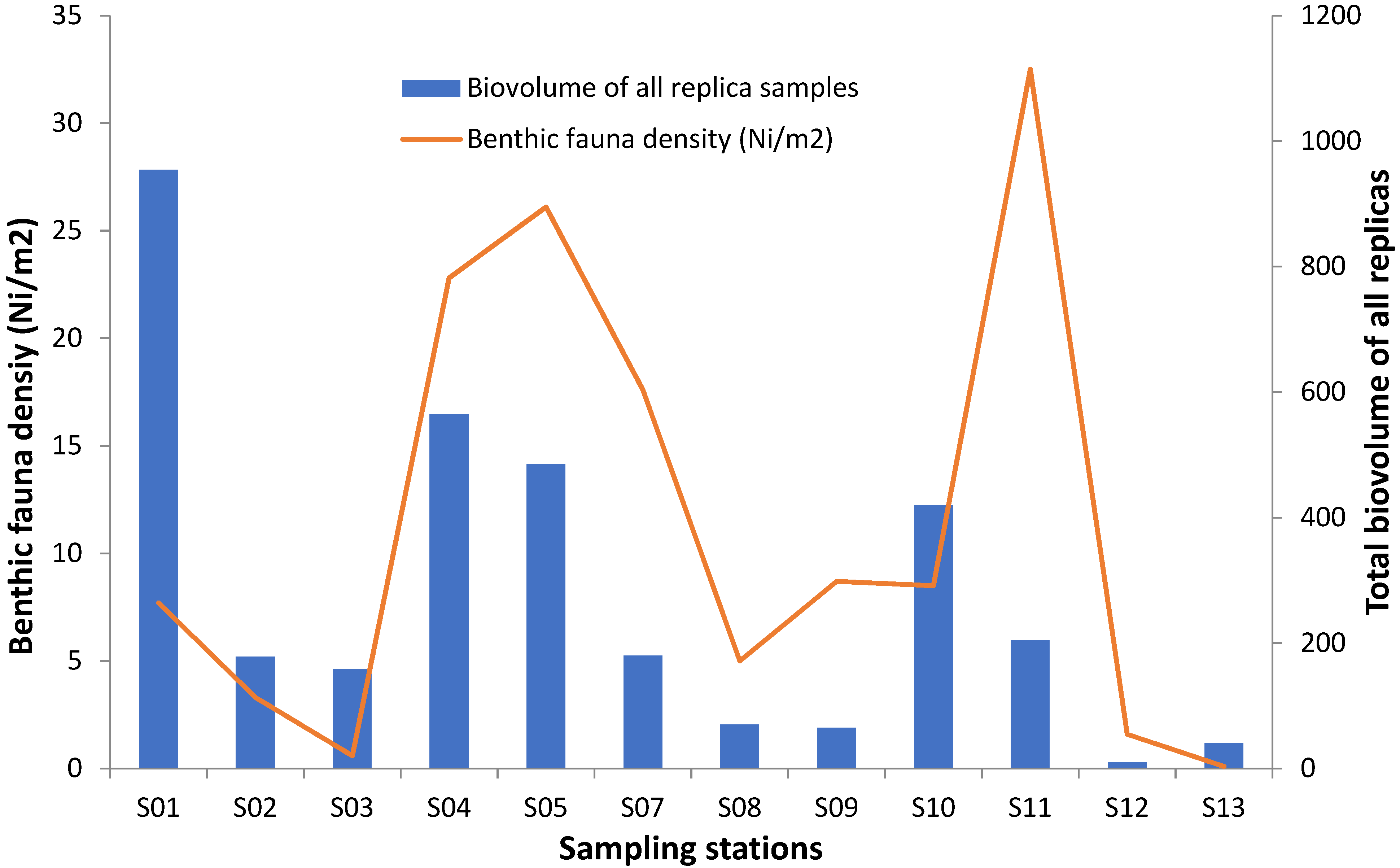
3.3. Evaluation of Dry Biomass, Living Biovolumes, and Densities

The total biovolume of all replicates varied from 10.0 to 953.58 mL (Figure 2,

Table 3. Estimations of the dry biomass, percentage of debris, real biovolume, and the density of benthic fauna at the 13 sampling stations located along the maritime canal connecting Ziguinchor port to the sea.

Stations	Biovolume of All Samples (mL)	Percentage (%) of Debris	Dry Biomass (mL)	Real Biovolume (mL)	Densities (Nind/m2)
S01	953.85	95	906.16	47.69	7.70
S02	178.0	93	165.5	12.46	3.31
S03	158.0	98	154.84	3.16	0.60
S04	565.0	97	548.05	16.95	22.80
S05	485.0	97	470.45	14.55	26.10
S06					0
S07	180.0	93	167.4	12.6	17.60
S08	70.0	95	63.0	7.0	5.00
S09	65.0	98	63.7	1.3	8.70
S10	420.0	98	411.6	8.4	8.50
S11	205.0	97	198.85	6.15	32.50
S12	10.0	98	9.8	0.2	1.60
S13	40.0	98	39.2	0.8	0.10

). The total biovolume was higher at Station 1 (953.85 mL) (t-test: p < 0.001), followed by Stations 4 (565.0 mL), 5 (485.0 mL), and 10 (420.0 mL) and lower at Stations 12 (10.0 mL), 13 (40.0 mL), 9 (65.0 mL), and 8 (70.0 mL) (Figure 2, Table 3). The percentage of debris (dry matter), estimated from the total biomass, varied from 93 to 98% (Table 3). The dry biomass varied from 9.8 (Station 12) to 906.16 (Station 1). It was higher at Station 1, followed by Stations 4 (548.05), 5 (470.45), and 10 (411.6). It was lower at Stations 12 (9.8), 13 (39.2), 9 (63.0), and 8 (63.7) (Table 3). The real biovolume, determined by taking into account the percentages of debris and other residues, varied between 0.20 and 47.69. The most abundant biovolume was recorded at Station 1 (47.69), followed by Stations 4 (16.95), 5 (14.55), 7 (12.60), and 2 (12.46). Least abundant biovolumes were recorded at Stations 12 (0.2) and 13 (0.8). There was a complete absence of benthic fauna at S6. The benthic fauna density, reported in the number of benthic animals per m², varied between 0.10 and 32.5 ind/m² (Figure 2, Table 3). The highest density was recorded at Station 11 (32.50 ind/m²), followed by Station 5 (26.1 ind/m²) and 4 (22.8 ind/m²). The lowest densities were recorded at Stations 13 (0.10) and 3 (0.60) (Figure 2).

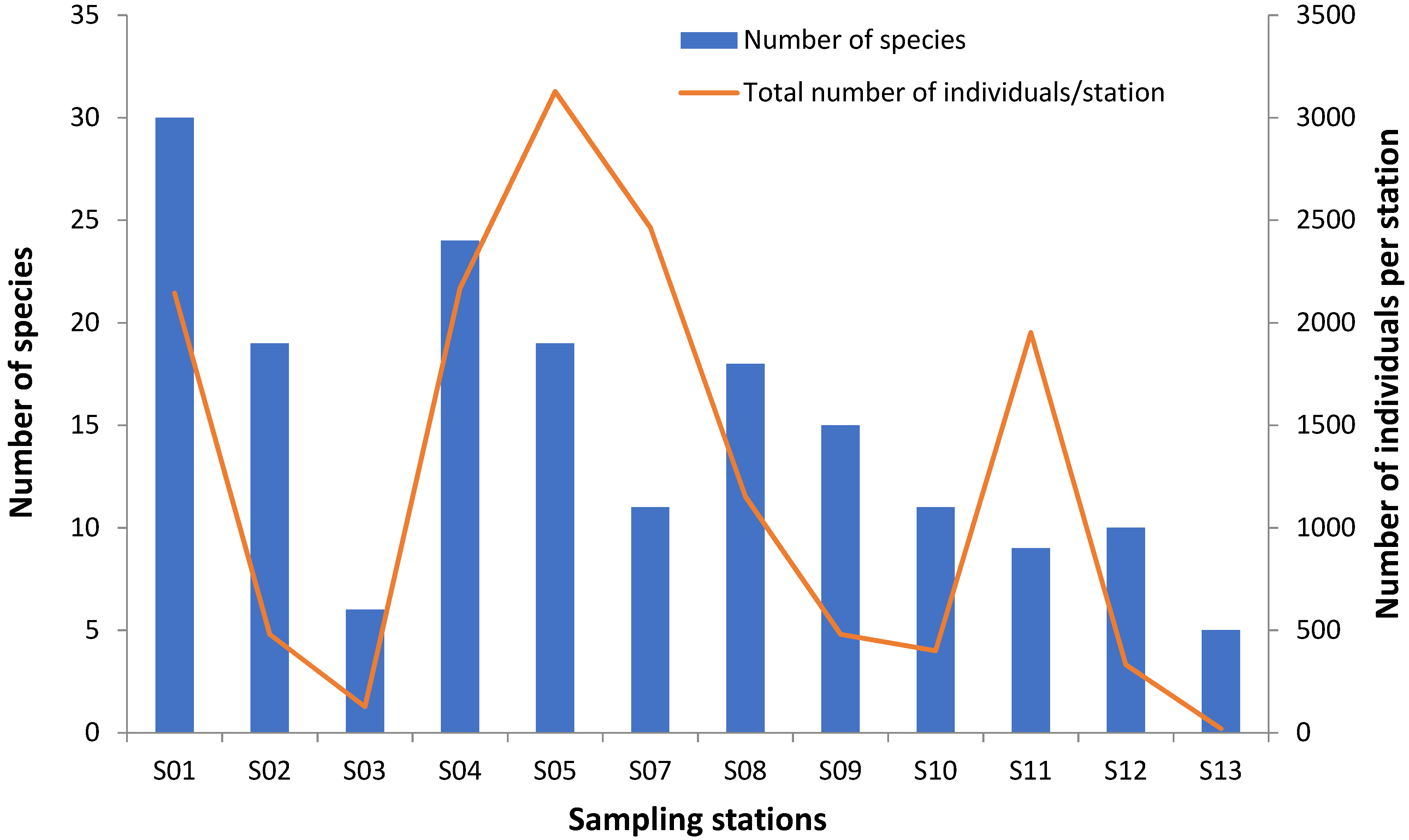
3.4. Species Abundance

Species abundance varied from 20 (Station 13) to 3128 individuals (Station 5) (Figure 3,

Table 4. Diversity and evenness of benthic wildlife at the thirteen sampling stations (1 to 13) of the road channel from the mouth of the Casamance estuary to Ziguinchor.

Stations	Number of Species	Total Number of Individuals/Station	Shannon-Wiener Index	Pielou Index
S01	30	2144	2.772	0.092
S02	19	480	2.671	0.141
S03	6	127	1.494	0.249
S04	24	2168	2.446	0.101
S05	19	3128	2.473	0.13
S06
S07	11	2464	1.279	0.116
S08	18	1152	2.44	0.071
S09	15	480	2.19	0.163
S10	11	400	2.227	0.202
S11	9	1952	0.77	0.085
S12	10	332	1.407	0.141
S13	5	20	1.557	0.311

). Species abundance was higher at S5, S7, S4, S1, S8, and S11 and lower at S2, S3, S9, S10, S12, and S13 (Figure 3, Table 4). The richest and most diversified sampling stations were those closest to the bolon and those located on river banks (Figure 1, Figure 3). Stations 1 and 4, located near Ziguinchor, had the highest diversity (30 and 24 species, respectively) (Figure 3). It was found that sampling stations closer to the estuary mouth were lower in species richness.

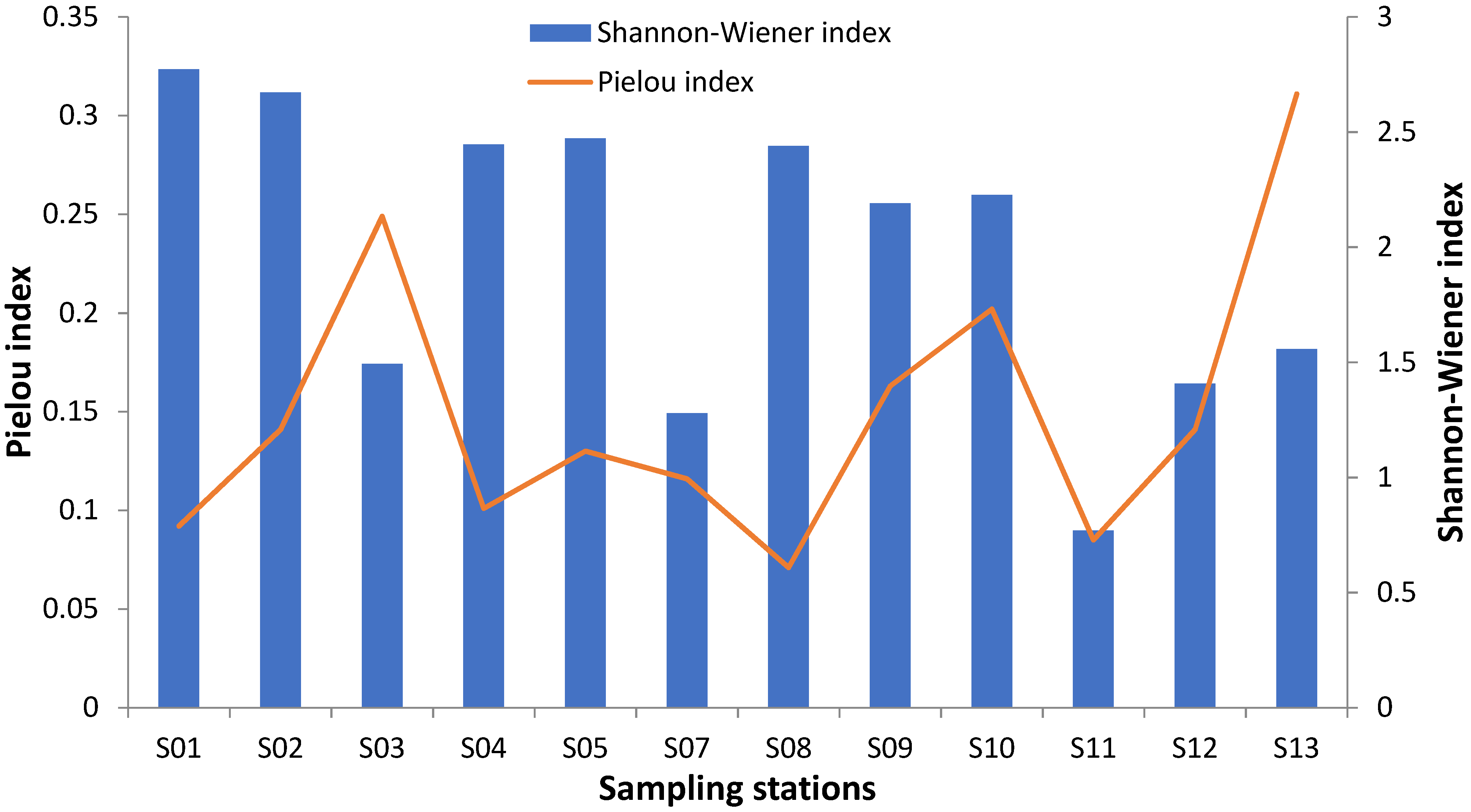
3.5. Shannon-Weaver and Pielou Indexes

The benthic biodiversity per station, measured using the Shannon-Weaver index, is indicated in Figure 4 and Table 4. The average Shannon index varied significantly between 0.770 and 2.772 (t-test: t = 6.2332; df = 803; p = 7.375 × 10⁻¹⁰). The highest values were observed at Stations 1 and 2, followed by Stations 5, 4, and 8 (Figure 4, Table 4). The index was lower at Station 11 (Figure 4, Table 4). The Pielou index per station, calculated from the ratio of the average Shannon indexes and the number of species, are indicated in Figure 4 and Table 4. The Pielou index varied significantly between 0.07 and 0.33 (t-test: t = 6.2332; df = 803; p = 7.375 × 10⁻¹⁰). The highest Pielou indexes were recorded at Stations 13, 3, and 10, while the lowest were observed at Stations 11 and 8. The equability index was null at Station 6 (Figure 4, Table 4).

3.6. Trophic Groups and Spatial Distribution

Several zoological groups were thus observed based on various guides for the trophic classification of benthic fauna (

Table 5. Trophic groups of the benthic wildlife found at the 13 sampling locations along the road channel connecting the Ziguinchor maritime port to the sea.

Trophic Groups	S01	S02	S03	S04	S05	S07	S08	S09	S10	S11	S12	S13
Omnivores	240			520	416	1344
Filter feeders	240	32		288	312			68	16	1632	212	12
Detritus feeders		56	8	80	16			4			16
Filter feeder & Detritivores	32				288
Carnivores	96	64		8	304		48	56		48
Necrophagous	176			136		64		88				2
Carnivores & Detritivores	240			8	16	32	16
Bottom deposit feeders	16
Detritivores & Herbivores	16
Detritivores & Omnivores	16
Suspension feeders	480			72	232	32	64		48		12
Zooplankton feeders	16	32		480		768	48	16				6
Plankton & Nutriment feeder	32	8			384	32		48			12

). These include macrophage carnivores, comprised of wandering polychaetes, gastropods, and decapods; necrophages; macrophages (gastropods and decapods); macrophage detritivores (amphipods, isopods, tanaidaceae, decapods, polychaetes, nereids, crustaceans, and bivalve mollusks); filter feeders (bivalve mollusks); and microphage suspensivores (bivalve mollusks, crustaceans, and annelids). Among these trophic groups are also bottom deposit feeders, detritivore-herbivores, detritivore-omnivores, and detritus feeders (Table 5). The benthic fauna of the Casamance estuary was dominated by the carnivores, filter feeders, and detritus feeders. The sampling station with the most trophic groups is S01, located upstream from the estuary (Table 5). However, other sampling stations with a relatively high number of trophic groups are also found upstream and downstream from the estuary and at midstream. This is the case for S02, S04, S05 (estuary upstream), S07 (estuary midstream), and S09 (estuary downstream) (Table 5).

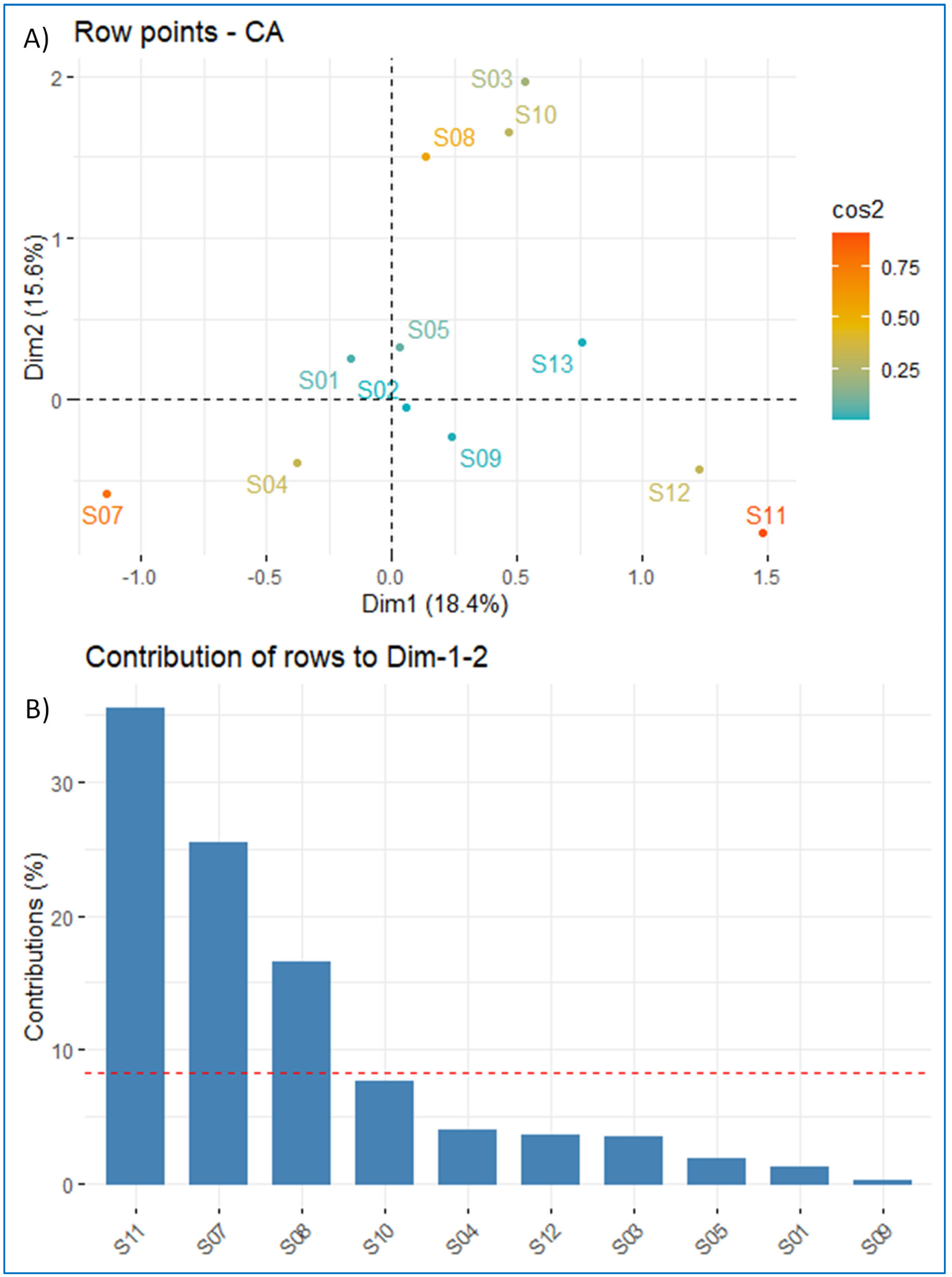
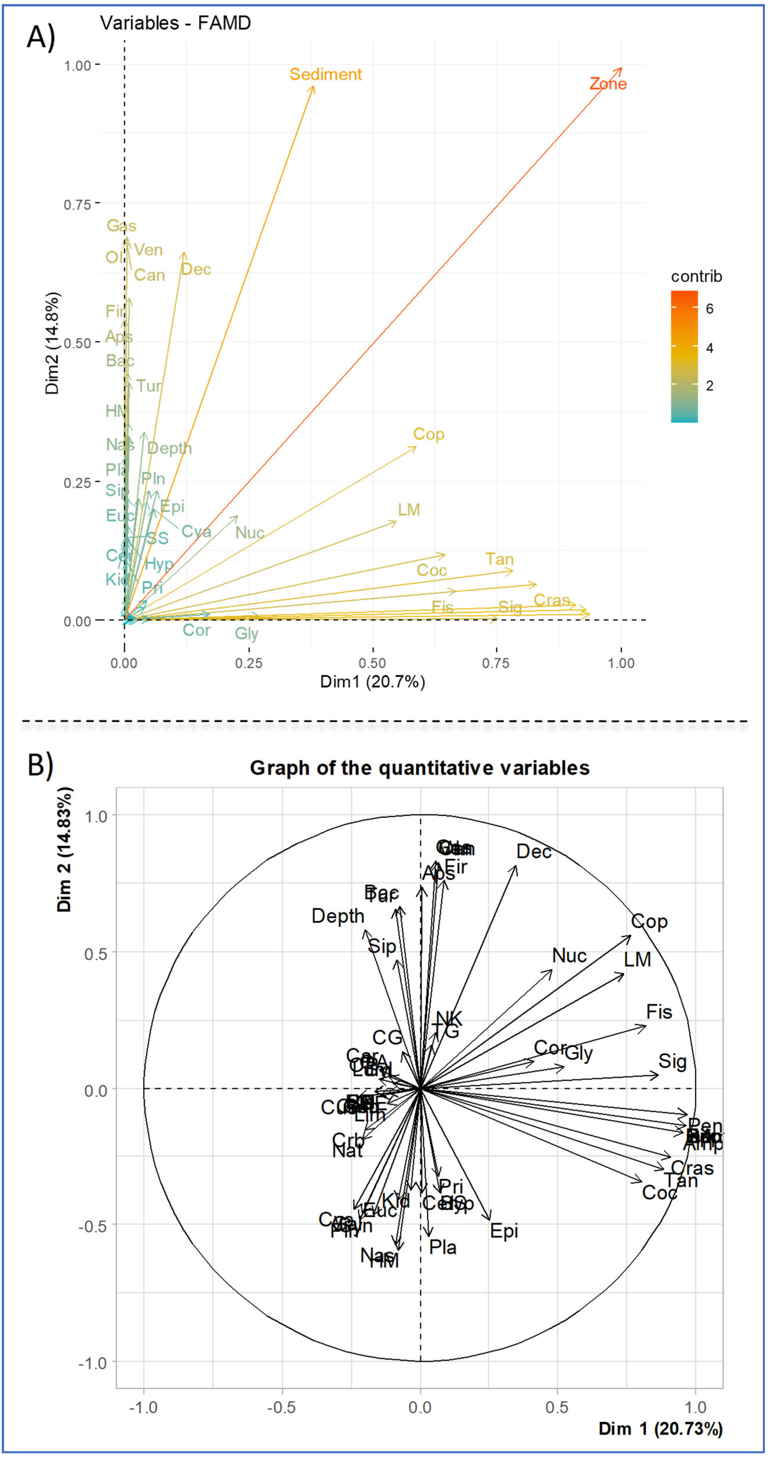
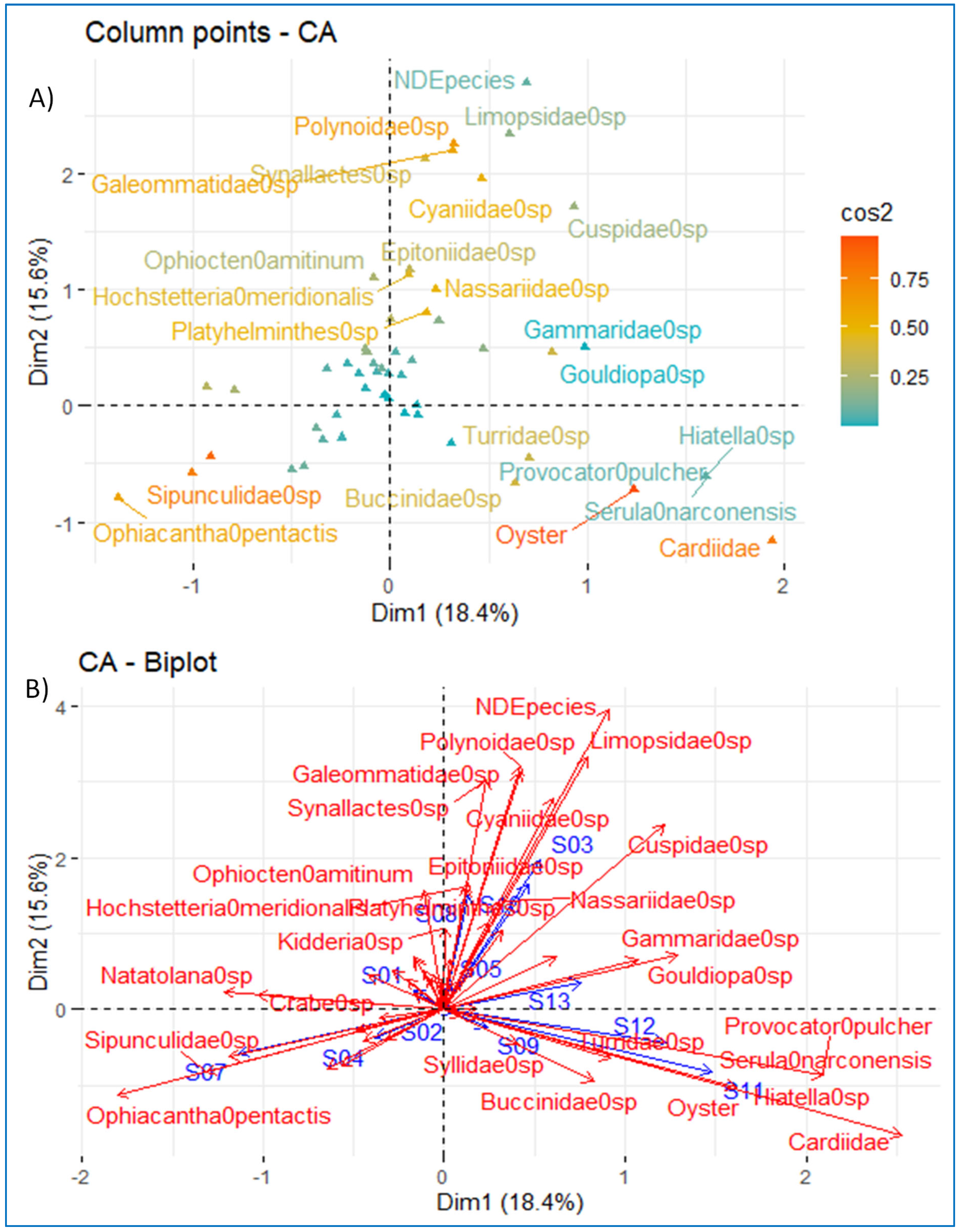
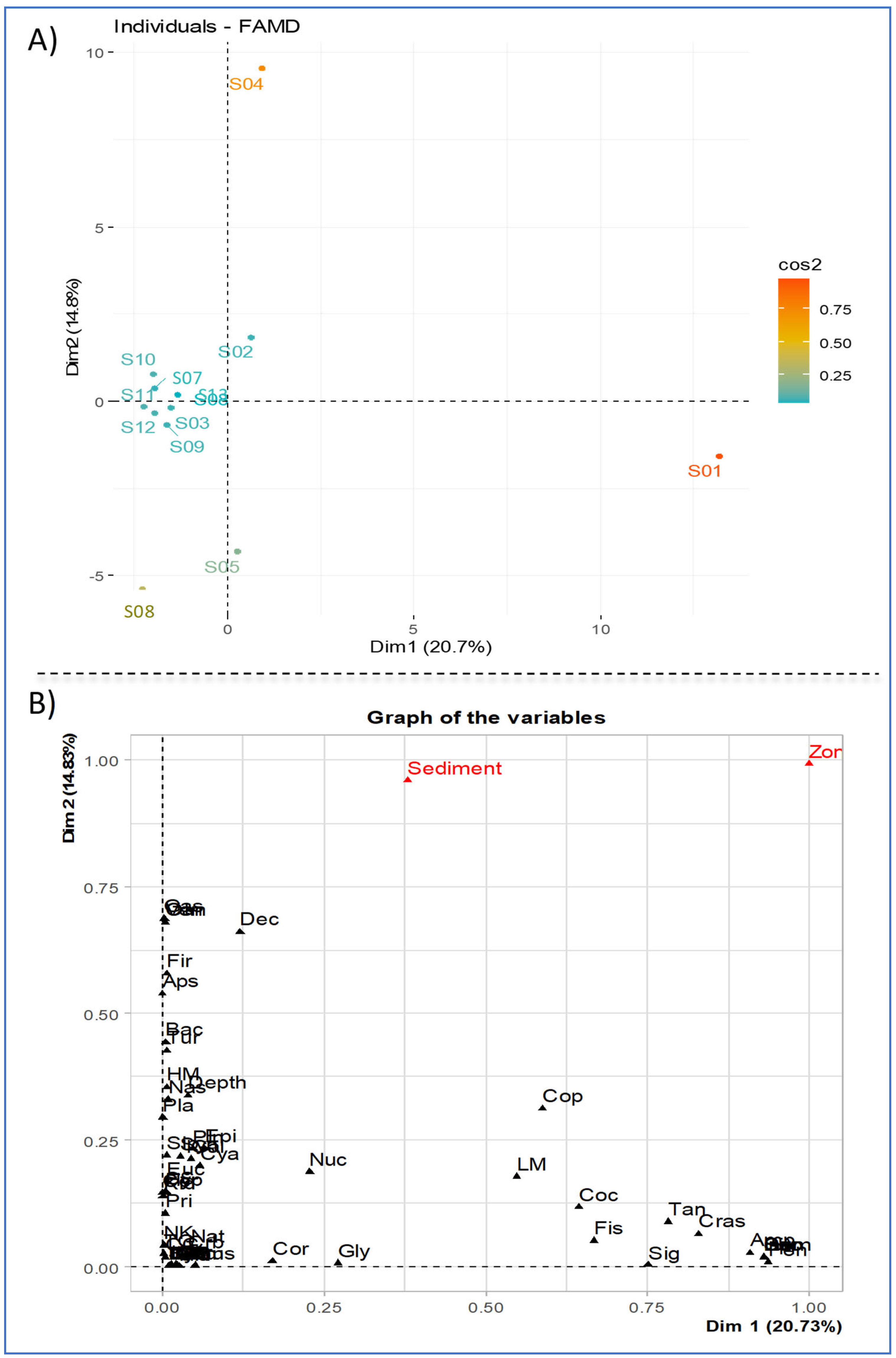
3.7. Correspondence Factorial Analysis (CFA) and Factor Analysis for Mixed Data (FAMD)

Correspondence factorial analysis (CFA) showed that 34% of the total inertia was explained by the first two axes (Dim 1 = 15.6% and Dim 2 = 18.4%) (Figure 5). Figure 5A shows that all stations are well-represented on the two dimensions, particularly S07, S11, and S08. The Figure 5A also shows that the stations are separated into four groups or clusters: Group 1 (S07 and S04), Group 2 (S01, S02, S05, S09, and S13), Group 3 (S03, S08, and S10), and Group 4 (S12 and S09). The red dashed line in Figure 5B indicates the expected mean value. Any station with a value greater than this has a large contribution of lines to the various dimension poles. Figure 6A shows repartition of benthic fauna species on the two dimensions of the factorial plan. Any variable with a value higher than the mean value has a positive contribution of columns to the different poles of the dimensions (Supplementary Materials). Thus, there are only eight species that contribute well to the poles of both dimensions: oyster Crassostrea gasar, Cardiidae sp., Sipunculidae sp., Polynoidae sp., Galeommatidae sp., Cyaniidae sp., Nassariidae sp., and Platyhelminthes sp. (Figure 6A, Supplementary Materials).

Group 1 is characterized by Ophiacantha pentactis and Sipunculidae sp., and to a lesser extent, Natalano sp. and Lithodes murrayi (Crab sp.), whereas Group 2 is mainly characterized by Kidderia sp., Platyhelminthes sp., Epitoniidae sp., Syllidae sp., Nassariidae sp., Buccinidae sp., Gammaridae sp., and Goudiopa sp. (Figure 6B). Group 3 is marked by Polynoidae sp., Limopsidae sp., Geommatidae sp., Cyaniidae sp., Cuspidae sp., and EDSpecies (undetermined species), and Group 4 by Turridae sp., Provocator pucher, Serula narconensis, Hiatella sp., Crassostrea gasar (oyster), and Cardiidae sp. (Figure 6B).

The FAMD including the depth, sediment type, and the estuarine zone of the sampling sites showed that 35.5% of the total inertia was explained by the first two axes (Dim 1 = 20.8% and Dim 2 = 14.7%) (Figure 7A,B). The sampling locations S02, S03, S07, S09, S10, S11, S12, and S13 are gathered in the same group, which is isolated from the second group formed by locations S08 and S05. Locations S01 and S04 are isolated from these groups and from each other (Figure 7A). Figure 7B shows the plots of species, the depth, and qualitative variables (sediment type and estuarine zone) on the factorial plan. The distribution of species is not correlated to the estuarine zone, which refers to the locations of the sampling stations (Figure 8A). However, the distribution of certain species, such as Gas (Gasteropoda sp.), Ven (Veneroida sp.), Ol (Ophiacantha imago), Dec (Decapoda sp.), Fir (Fissurellidae sp.), Aps (Apseudomorpha sp.), Tur (Turridae sp.), Nas (Nassariidae sp.), HN (Hochstetteria meridionalis), Pln (Polynoidae sp.), Pla (Platyhelminthes sp.), and Sip (Sipunculidae sp.) was corrected with the sediment type and the depth of the sampling stations (Figure 8A,B). On the other hand, the distribution and abundance of species, such as Tan (Tanaidacea sp.), Coc (Coryceaus sp.), Sig (Sigalionidae sp.), Cras (Crassatellidae sp.), Cor (Corals), Gly (Glyceridae sp.), and Cop (Copepoda sp.) are not correlated to these variables (Figure 8A,B).

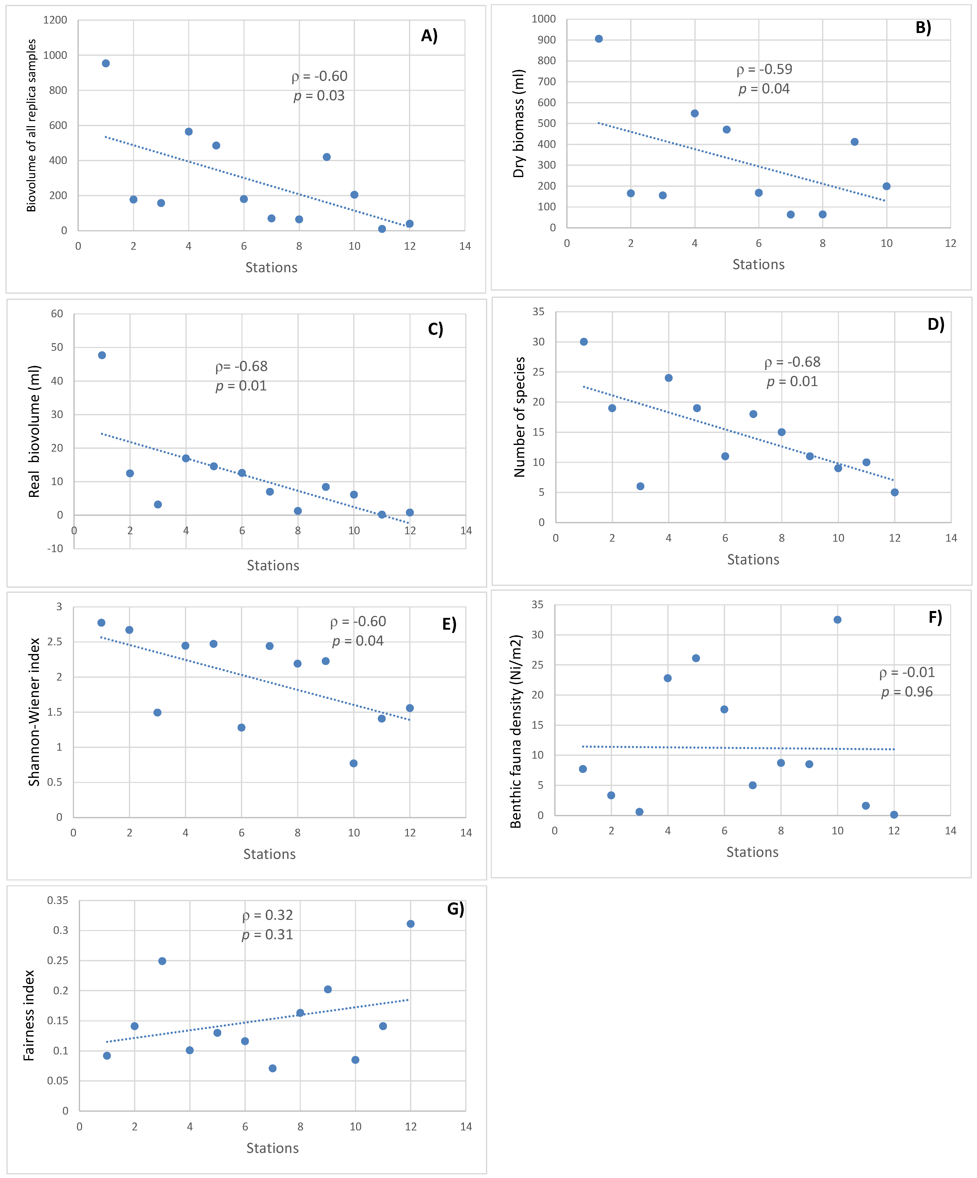
3.8. Correlation Results

A significant negative correlation between the total biovolumes of all replicate samples (Spearman rank correlation: ρ = −0.60; p = 0.03, respectively), dry biomass (Spearman rank correlation: ρ = −0.59; p = 0.04, respectively), and real biovolume of benthic fauna (Spearman rank correlation: ρ = −0.68; p = 0.01, respectively) and distance from the estuary mouth was detected (Figure 9A–C). Likewise, the number of species and the Shannon-Wiener index showed a significant negative correlation with geographic distance from the estuary mouth (Spearman rank correlation: ρ = 0.68; p = 0.01; ρ = 0.60; p = 0.04, respectively) (Figure 9D,E). The comparisons of the strength showed that the degree of correlations with the distance was higher for the real biomass (Figure 9C) and the total number of species per station (Figure 9D) compared to the biovolume of all replicate samples (Figure 9A) and the Shannon-Wiener index (Figure 9D). On the other hand, the benthic fauna density and the Pielou index did not show a significant correlation with the geographic distance (Spearman rank correlation: ρ = −0.01; p = 0.96; ρ = 0.32; p = 0.31, respectively) (Figure 9F,G).

4. Discussion

Spatial location is likely to influence the distribution, abundance, and species richness of benthic fauna [11,33,34,35,36]. In this study, the composition, density, abundance, and richness of benthic fauna varied significantly across the stations sampled. There is lots of variability in the dry biomass data, i.e., from 9.8 (S12) to 906.16 (S01). It appears that this variability has nothing to do with depth. Interestingly, the variability in the number of species and number of individuals per species show a similar pattern may explain the variability in the dry biomass data. Some of the sixty taxa collected at 13 sampling stations, such as Serula narconensis, Lumbrineridae sp., Syllidae sp., Ophiacantha imago, Ophiacantha pentactis, Synallactes sp., Euphausiacea sp., Cumacea sp., Serilis sp., Isopa sp., Cerithiopsidae sp., Inuncula sp., Cancellariidae sp., Gasteropoda sp., Epoitonidae sp., Bivalvia sp., Limopsidae sp., Cardiidae sp. are rare (present only in one station) and may be habitat specialists dominant in their niche, whose relative abundance may be the result of a localized disturbance or recruitment event [36]. The density of benthic fauna is very heterogeneous (01–32.5) with the highest values being recorded at Station 11. The high density at this station is essentially due to the abundance of oyster spat Crassostrea gasar, which largely dominates the species encountered at this location. The species richness decreases from upstream to downstream stations, which could be explained by higher current speeds in the estuary mouth area compared to the stations around Ziguinchor city (located 63 km from the mouth). The richest and more diversified sampling stations were those close to the bolon and those located on the estuary banks, which is probably due to the spatial heterogeneity of the circulation of water masses in this part of the estuary [37]. Physicochemical factors, such as depth and sediment type, have been identified as determinants in the composition and diversity of benthic communities in tropical estuarine ecosystems [38,39,40]. For example, soft muddy substrata with high organic content are usually colonized by deposit feeders, whereas sands or firm muds are generally inhabited by suspension feeders [41,42]. The results of this study show an apparent correlation between benthic community composition and sediment type, indicating that sediment properties are among the major causes of benthic faunal composition and clustering. Likewise, there is a clear relationship between benthic community composition and the depth gradient of the sampled stations, suggesting that this parameter influences the special distribution and abundance of benthic fauna. It is unlikely that the absence of benthic organisms at the Station 6 is due to the sediment type or the depth, since samples were collected from other stations with similar sediment type and depth. No benthic organism was collected during the replicate sampling operations performed at this station, suggesting that their absence is not due to a failure in the sampling operation. Moreover, the same sampling technique was used at all other stations, strongly supporting that the absence of benthic organisms in this location is not due to a technical problem during the sampling.

Salinity can also influence the occurrence, abundance, distribution, and diversity of benthic organisms in tropical estuaries. Indeed, the Casamance River is an inverse estuary with salinity that increases with the distance from the mouth (from downstream to upstream) [26,27]. This inverse salinity gradient results from limited freshwater inputs from river discharge and rainfalls and high evaporation rates [23,27] associated with the gentle slope, which causes saltwater intrusions into the estuary up to 200 km from its mouth. The results of this study show higher taxonomic composition, abundance, and richness of benthic species at the upstream stations, with higher salinities compared to the midstream and downstream stations. This suggests that differences in faunal diversity in the studied zones of this estuary might be due spatial variations in water salinity. However, these results are in contradiction with those of Debenay et al. [43], who showed a marked decrease of zooplankton and foraminifera from downstream to upstream of the Casamance estuary. In accordance with our results, a previous study by Ceesay et al. [38] conducted in the neighboring normal Gambia estuary (salinity increasing from upstream to downstream) showed that the taxonomic richness of benthic fauna increases from upstream to downstream stations. Ceesay [38] hypothesized that this may related to the reduced flows and increased habitat in the downstream part of the estuary. In the Gambia estuary, habitat heterogeneity favors the diversity of benthic fauna due to the abundance of food resources and the low presence of predators in the downstream section [38]. Other studies also report higher benthic fauna richness in mangrove forests due to higher available organic resources compared to unvegetated downstream zones [44,45,46]. The mangrove-derived organic resources thus constitute a major component in benthic food webs in estuarine ecosystems and can therefore influence the distribution patterns, including benthic fauna in estuarine ecosystems [47]. The availability of organic sources derived from the mangrove can lead to marked differences in benthic faunal composition, abundance, and diversity as well as in food webs The upstream area of the Casamance estuary may harbor food resources due to the presence of the mangrove, which may attract benthic fauna species. Although food availability was not analyzed in this study, this may explain the higher benthic faunal composition and diversity in upstream part of the estuary. The absence or loss of mangroves in the downstream zone of the estuary can lead to changes in benthic community composition.

Some taxa (Neanthes kerguelensis, Syllidae sp., Hyperiidea sp., Amphipodae sp., and Priapulidae sp.) may be habitat-specialist species dominant in their niche but unable to colonize and persist in other habitats. Indeed, they were rare but relatively abundant at the few stations where they were found. This relative abundance may be the result of a localized disturbance or recruitment event [36]. Indeed, road channel dredging in the Casamance estuary may cause changes in the habitats and migration of benthic species, which can lead to reduced reproductive success, reduced growth rate, or even death of benthic organisms at the early stage [35]. The absence of benthic fauna at Station 6 and the relative low diversity at Station 11 suggest that they might be environmentally sensitive areas inhabited by threatened species. The high species diversity at Stations 1, 2, 5, 4, and 8 indicate that these are ecologically important areas that can be damaged by the road channel construction and its utilization. Therefore, the habitat and fauna characterization in this study identifies the existence of potential ecologically important areas in this ecosystem that must be protected from dredging. Although results reported here may provide indications for appropriate management plans, spatial biodiversity changes should be regularly monitored. The responses of benthic fauna to physical habitat degradation and chemical contamination should be characterized through monitoring programs. These monitoring plans can include environmental health assessment studies based on benthic fauna diversity [48,49]. Such monitoring plans should include more sampling stations in those sectors surrounding the port and road channel, in order to increase the range of the study zone and to be able to identify ecologically important areas. The seasonal differences in this region cause significant variations in the physicochemical factors, which lead to changes in benthic fauna composition and distribution. For example, salinity, which is a determinant factor for the distribution of benthic fauna communities, varies largely between the dry season and the rainy season due to differences in freshwater inflows and evaporation rates between seasons [26,27,28]. The higher salinities in the dry season compared to the rainy season may cause significant temporal and spatial changes in the benthic fauna distribution.

5. Conclusions

The benthic fauna of the downstream section of the Casamance estuary presents a fairly significant specific diversity (60 species) and an almost regular distribution of bivalve mollusks, mainly the Crassostrea gasar oyster, which is locally the most exploited species. From the Shannon-Wiener and Pielou indexes, it appears that the benthic fauna of the estuary is fairly stable in a biological environment that is highly variable, especially for the salinity whose variations are linked to annual rainfall and evaporation rates. Macrophages (bivalve mollusks, gastropod mollusks, nematodes, crustaceans, and amphipods) represent nearly 68.91% of the fauna and can be used as biological indicators for monitoring the dredging impacts of the road channel (Casamance estuary) of Ziguinchor port. Sediment type, depth of the sampled stations, salinity, and mangrove forests appeared as important factors that influence the distribution and abundance of benthic fauna in the Casamance estuary. However, for further studies, other factors, such as temperature, pH, dissolved oxygen levels, and water quality (turbidity, pollution, etc.) may be determinant and should be taken into account in the monitoring plans. Indeed, these factors vary significantly between seasons (rainy season and dry season) and can therefore cause changes in the patterns of benthic fauna composition and distribution. Such variations may affect the availability of food sources for benthic fauna and lead to changes in benthic fauna distribution patterns (especially for mobile species). The monitoring plans for the preservation of the ecosystem health and biological diversity, especially benthic fauna biodiversity, should also take in consideration as well as the seasonal variations of rainfalls and related changes in the physicochemical factors. For example, salinity, which is a determinant factor for the distribution of benthic fauna communities, varies largely between the dry season and the rainy season due to differences in freshwater inflows and evaporation rates between seasons [26,27,28]. The higher salinities in the dry season compared to the rainy season may cause significant temporal and spatial changes in the benthic fauna distribution. Characterization of benthic fauna should be conducted regularly and extended to other sectors around the road channel and the port. This would allow the evaluation of long-term responses of benthic organisms to dredging activities and boat traffic, especially physical habitat modifications, changes in migration, and pollution pressure. Sampling campaigns should be regularly conducted to assess the degree of biodiversity loss or restoration and the environmental health status. The monitoring recommendations formulated in this study endeavor to aid local port management authorities to establish feasible, rapid, and cost-effective monitoring plans.

References

1. Baran, E. Biodiversity of Estuarine Fish Faunas in West Africa; Naga, The ICLARM Quarterly: Metro Manila, Philippines, 2000; Volume 23. [Google Scholar]
2. Cloern, J.; Jassby, A. Drivers of change in estuarine-coastal ecosystems: Discoveries from four decades of study in San Francisco Bay. Rev. Geophys. 2012, 50, 1–33. [Google Scholar] [CrossRef] [Green Version]
3. Dolbeth, M.; Cardoso, P.G.; Grilo, T.F.; Bordalo, M.D.; Raffaelli, D.; Pardal, M.A. Long-Term Changes in the Production by Estuarine Macrobenthos Affected by Multiple Stressors. Estuar. Coast. Shelf Sci. 2011, 92, 10–18. [Google Scholar] [CrossRef]
4. Villanueva, M.C. Contrasting tropical estuarine ecosystem functioning and stability: A comparative study. Estuar. Coast. Shelf Sci. 2015, 155, 89–103. [Google Scholar] [CrossRef] [Green Version]
5. Elliott, M.; Whitfield, A.K. Challenging paradigms in estuarine ecology and management. Estuar. Coast. Shelf Sci. 2011, 94, 306–314. [Google Scholar] [CrossRef]
6. McLusky, D.; Elliott, M. The Estuarine Ecosystem: Ecology, Threats, and Management. In Elliott Threats and Management; McLusky, M.D.S., Ed.; Oxford University Press: Oxford, UK, 2004. [Google Scholar]
7. Edgar, G.J.; Barrett, N.S.; Graddon, D.J.; Last, P.R. The conservation significance of estuaries: A classification of Tasmanian estuaries using ecological, physical and demographic attributes as a case study. Biol. Conserv. 2000, 92, 383–397. [Google Scholar] [CrossRef]
8. Edgar, G.J.; Barrett, N.S.; Last, P.R. The Distribution of Macroinvertebrates and Fishes in Tasmanian Estuaries. J. Biogeogr. 1999, 26, 1169–1189. [Google Scholar] [CrossRef]
9. Grizzetti, B.; Passy, P.; Billen, G.; Bouraoui, F.; Garnier, J.; Lassaletta, L. The role of water nitrogen retention in integrated nutrient management: Assessment in a large basin using different modelling approaches. Environ. Res. Lett. 2015, 2015, 10. [Google Scholar] [CrossRef]
10. Trombulak, S.C.; Frissell, C.A. Review of ecological effects of roads on terrestrial and aquatic communities. Conserv. Biol. 2000, 14, 18–30. [Google Scholar] [CrossRef]
11. Chatzinikolaou, E.; Mandalakis, M.; Damianidis, P.; Dailianis, T.; Gambineri, S.; Rossano, C.; Scapini, F.; Carucci, A.; Arvanitidis, C. Spatio-temporal benthic biodiversity patterns and pollution pressure in three Mediterranean touristic ports. Sci. Total Environ. 2017, 624, 648–660. [Google Scholar] [CrossRef]
12. Blanchard, A.L.; Feder, H.M. Adjustment of benthic fauna following sediment disposal at a site with multiple stressors in Port Valdez, Alaska. Mar. Pollut. Bull. 2003, 46, 1590–1599. [Google Scholar] [CrossRef]
13. Boyd, W.A.; Brewer, S.K.; Williams, P.L. Altered behaviour of invertebrates living in polluted environments. In Behavioural Ecotoxicology; Dell’Omo, G., Ed.; John Wiley & Sons: Chichester, UK, 2002. [Google Scholar]
14. Kravitz, M.J.; Lamberson, J.O.; Ferraro, S.P.; Swartz, R.C.; Boese, B.L.; Specht, D.T. Avoidance response of the estuarine amphipod Eohaustorius estuarius to polycyclic aromatic hydrocarbon-contaminated, field-collected sediments. Environ. Toxicol. Chem. 1999, 18, 1232–1235. [Google Scholar] [CrossRef]
15. Scarlett, A.; Canty, M.N.; Smith, E.L.; Rowland, S.J.; Galloway, T.S. Can Amphipod Behavior Help to Predict Chronic Toxicity of Sediments? Hum. Ecol. Risk Assess. Int. J. 2007, 13, 506–518. [Google Scholar] [CrossRef]
16. Reddy, C.M.; Eglinton, T.I.; Hounshell, A.; White, H.K.; Xu, L.; Gaines, R.B.; Frysinger, G.S. The West Falmouth oil spill after thirty years: The persistence of petroleum hydrocarbons in marsh sediments. Environ. Sci. Technol. 2002, 36, 4754–4760. [Google Scholar] [CrossRef]
17. Reimer, J.D.; Yang, S.Y.; White, K.N.; Asami, R.; Fujita, K.; Hongo, C.; Ito, S.; Kawamura, I.; Maeda, I.; Mizuyama, M.; et al. Effects of causeway construction on environment and biota of subtropical tidal flats in Okinawa, Japan. Mar. Pollut. Bull. 2015, 94, 153–167. [Google Scholar] [CrossRef] [PubMed]
18. Baudin, F.; Disnar, J.R.; Martinez, P.; Dennielou, B. Distribution of the organic matter in the channel-levees systems of the Congo mud-rich deep-sea fan (West Africa). Implication for deep offshore petroleum source rocks and global carbon cycle. Mar. Pet. Geol. 2010, 27, 995–1010. [Google Scholar] [CrossRef] [Green Version]
19. Friedlander, A.M.; Ballesteros, E.; Fay, M.; Sala, E. Marine Communities on Oil Platforms in Gabon, West Africa: High Biodiversity Oases in a Low Biodiversity Environment. PLoS ONE 2014, 9, e103709. [Google Scholar] [CrossRef]
20. Ober, H.K. Effects of Oil Spills on Marine and Coastal Wildlife; UF/IFAS Extension WEC 285; Wildlife Ecology and Conservation Department: Gainesville, FL, USA; North Florida Research and Education Center (NFREC): Quincy, FL, USA, 2010. [Google Scholar]
21. Pradella, N.; Fowler, A.M.; Booth, D.J.; Macreadie, P.I. Fish assemblages associated with oil industry structures on the continental shelf of northwestern Australia. J. Fish Biol. 2013, 84, 247–255. [Google Scholar] [CrossRef]
22. DPZ. Groundbreaking at Ziguinchor Port Marks Important Economic Milestone; Degla, R., Ed.; Project Manager: Dakar, Senegal, 2010. [Google Scholar]
23. Thiam, E.; Singh, V. Space-time-frequency analysis of rainfall, runoff and temperature in the Casamance River basin, southern Senegal, West Africa. Water SA 2002, 28, 259–270. [Google Scholar] [CrossRef] [Green Version]
24. Saos, J.-L.; Bouteiller, C.; Diop, S. Aspects Géologiques et Géomorphologiques de la Casamance: Étude de la Sédimentation Actuelle. Rev. D’hydrobiologie Trop. 1987, 20 (3–4), 219–232. [Google Scholar]
25. FAO. The State of the World’s Biodiversity for Food and Agriculture; Bélanger, J., Pilling, D., Eds.; FAO Commission on Genetic Resources for Food and Agriculture Assessments: Rome, Italy, 2019; 572p, Licence: CC BY-NC-SA 3.0 IGO; Available online: https://www.fao.org/3/CA3129EN/CA3129EN.pdf (accessed on 12 May 2022).
26. Mikhailov, V.; Isupova, M. Hypersalinization of river estuaries in West Africa. Water Resour. 2008, 35, 367–385. [Google Scholar] [CrossRef]
27. Savenije, H.; Pagès, J. Hypersalinity: A dramatic change in the hydrolog of Sahelian estuaries. J. Hydrol. 1992, 135, 157–174. [Google Scholar] [CrossRef]
28. Pages, J.; Citeau, J.E.; Demarcq, H. Bathymétrie par imagerie spot sur la Casamance (Sénégal). Résultats préliminaires. In Proceedings of the International Colloqium on Spectral Signatures of Objects in Remote Sensing Held at Aussois, Modane, France, 18–22 January 1988; pp. 387–392. [Google Scholar]
29. Hibberd, T.; Moore, K. Field Identification Guide to Heard Island and McDonald Islands Benthic Invertebrates: A Guide for Scientific Observers Aboard Fishing Vessels; Fisheries Research and Development Corporation: Canberra, Australia, 2019; 159p, Available online: https://www.ccamlr.org/en/document/publications/field-identification-guide-heard-island-and-mcdonald-islands-benthic (accessed on 12 May 2022).
30. Grall, J.; Hilly, C. Tratement des Données Stationnelles (Faune); 2003; 2010p. Available online: http://www.rebent.org//medias/documents/www/contenu/pdf/document/Fiches_techniques/FT10-2003-01.pdf (accessed on 12 May 2022).
31. Gaudêncio, M.J.; Cabral, H.N. Cabral Trophic structure of macrobenthos in the Tagus estuary and adjacent coastal shelf. Hydrobiologia 2007, 587, 241–251. [Google Scholar] [CrossRef]
32. Dray, S.; Dufour, A.-B. The ade4 Package: Implementing the Duality Diagram for Ecologists. J. Stat. Softw. 2007, 22, 1–20. [Google Scholar] [CrossRef] [Green Version]
33. Diouf, P.S.; Diallo, A. Variations spatio-temporelles du zooplancton d’un estuaire hyperhalin: La Casamance. Rev. D’hydrobiologie Trop. 1987, 20, 257–269. [Google Scholar]
34. Akaahan, T.; Manyi, M.M.; Azua, E. Variation of Benthic Fauna Composition in River Benue at Makurdi, Benue State, Nigeria. Int. J. Fauna Biol. Stud. 2016, 3, 71–76. [Google Scholar]
35. Gutperlet, R.; Capperucci, R.M.; Bartholomä, A.; Kröncke, I. Benthic biodiversity changes in response to dredging activities during the construction of a deep-water port. Mar. Biodivers. 2015, 45, 819–839. [Google Scholar] [CrossRef]
36. Nephin, J.; Juniper, S.K.; Archambault, P. Diversity, abundance and community structure of benthic macro- and megafauna on the Beaufort Shelf and Slope. PLoS ONE 2014, 9, e101556. [Google Scholar] [CrossRef]
37. Millet, B. Caractéristiques de la marée dans l’estuaire de la Casamance: Etalonnage et Analyse harmonique d’enregistrements courantographiques de longue durée à Zigunichor. CRODT Doc. Sci. N 1991, 123, 12. [Google Scholar]
38. Ceesay, A.; Konan, Y.A.; Njie, E.; Koné, T. Diversity and spatial variation of benthic macroinvertebrates in the River Gambia estuary, West Africa. Int. J. Fish. Aquat. Stud. 2019, 7, 83–88. [Google Scholar]
39. Graca, B.; Burska, D.; Matuszewska, K. The impact of dredging deep pits on organic matter decomposition in sediments(Article). Water Air Soil Pollut. 2004, 158, 237–259. [Google Scholar] [CrossRef]
40. Kumar, P.S.; Khan, A. The distribution and diversity of benthic macroinvertebrate fauna in Pondicherry mangroves, India. Aquat. Biosyst. 2013, 9, 15. [Google Scholar] [CrossRef] [PubMed] [Green Version]
41. Desjardins, P.; Buatois, L.; Mangano, M. Tidal Flats and Subtidal Sand Bodies. Dev. Sedimentol. 2012, 10, 529–561. [Google Scholar] [CrossRef]
42. Herman, P.; Middelburg, J.; Heip, C. Benthic community structure and sediment processes on an intertidal flat: Results from the ECOFLAT project. Cont. Shelf Res. 2001, 21, 2055–2071. [Google Scholar] [CrossRef]
43. Debenay, J.P.; Pagès, J.; Diouf, P.S. Ecological zonation of the hyperhaline estuary of the Casamance river (Senegal): Foraminifera, zooplanktoon and abiotic variables. Hydrobiologia 1989, 174, 161–176. [Google Scholar] [CrossRef]
44. Bernardino, A.F.; Gomes, L.E.O.; Hadlich, H.L.; Andrades, R.; Correa, L.B. Mangrove clearing impacts on macrofaunal assemblages and benthic food webs in a tropical estuary. Mar. Pollut. Bull. 2018, 126, 228–235. [Google Scholar] [CrossRef]
45. Bissoli, L.; Bernardino, A. Benthic macrofaunal structure and secondary production in tropical estuaries on the Eastern Marine Ecoregion of Brazil. PeerJ 2018, 6, e4441. [Google Scholar] [CrossRef] [Green Version]
46. Kristensen, E. Mangrove crabs as ecosystem engineers; with emphasis on sediment processes. J. Sea Res. 2008, 59, 30–43. [Google Scholar] [CrossRef]
47. Covich, A.; Palmer, M.; Crowl, T. The Role of Benthic Invertebrate Species in Freshwater Ecosystems. Bioscience 1999, 49, 119–127. [Google Scholar] [CrossRef] [Green Version]
48. Gray, J.; Elliott, M. Ecology of Marine Sediments: Science to Management; OUP: Oxford, UK, 2009; 260p. [Google Scholar]
49. Olsgard, F.; Gray, J.S. A comprehensive analysis of the effects of offshore oil and gas exploration and production on the benthic communities of the Norwegian continental shelf. Mar. Ecol. Prog. Ser. 1995, 122, 277–306. [Google Scholar] [CrossRef]
Figure 1. Map showing the benthic fauna sampling stations along the road channel of the Casamance estuary.
Conservation 02 00025 g001
Figure 2. Biovolume of all replicates and benthic fauna diversity for the different sampling stations.
Conservation 02 00025 g002
Figure 3. Number of species and total number of species per station for the different sampling stations.
Conservation 02 00025 g003
Figure 4. Shannon-Wiener index and Pielou index of benthic fauna for the different sampling stations.
Conservation 02 00025 g004
Figure 5. Correspondence factorial analysis (CFA) results of the benthic fauna collected in the thirteen sampling stations of the Casamance estuary: (A) represents the plot of sampling stations on the CFA plan and (B) represents the contribution of different stations.
Conservation 02 00025 g005
Figure 6. (A) Correspondence factorial analysis (CFA) results showing the distribution of benthic species and (B) correlation between sampling stations and species on the dissensions 1 and 2 of the factorial plan.
Conservation 02 00025 g006
Figure 7. (A) Factorial analysis for mixed data (FAMD) showing the plots of sampled stations and, (B) the plots of species and variables (depth, sediment types, and estuarine zones) of the sampled stations.
Conservation 02 00025 g007
Figure 8. (A) Factorial analysis for mixed data (FAMD) showing the distribution of the species in relation to sediment type, station depth, and estuarine zone, and (B) correlation circle.
Conservation 02 00025 g008
Figure 9. Relationships between (A) the total biovolume of all replicate samples, (B) dry biomass, (C) real biomass, (D) total number of species per station, (E) Shannon-Wiener index, (F) density, and (G) fairness index and the distance of sampling stations.
Conservation 02 00025 g009