Soil Consolidation Analysis in the Context of Intermediate Foundation as a New Material Perspective in the Calibration of Numerical–Material Models


Abstract
:1. Introduction
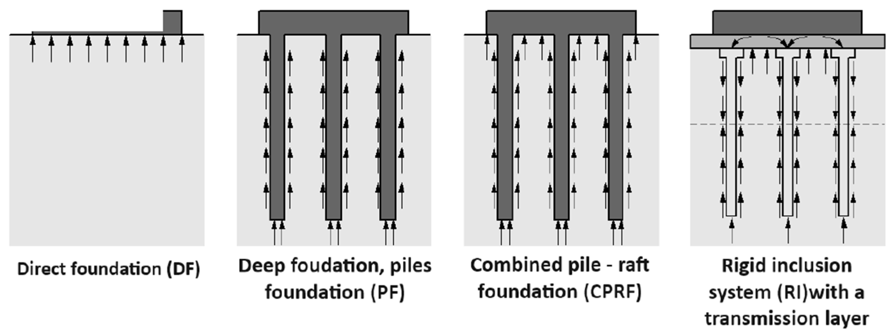
- Foundations founded directly (footings or slabs) on load-bearing and low-deformation soils;
- Indirect (deep) foundations based on lower layers of load-bearing soils, in the form of a certain number of piles or piles connected to the structure by a cap (grate, footing, slab) to transfer loads.
2. Materials and Methods—Background Information
3. Effect of Soil Consolidation on the Total Settlement of a Single Pile
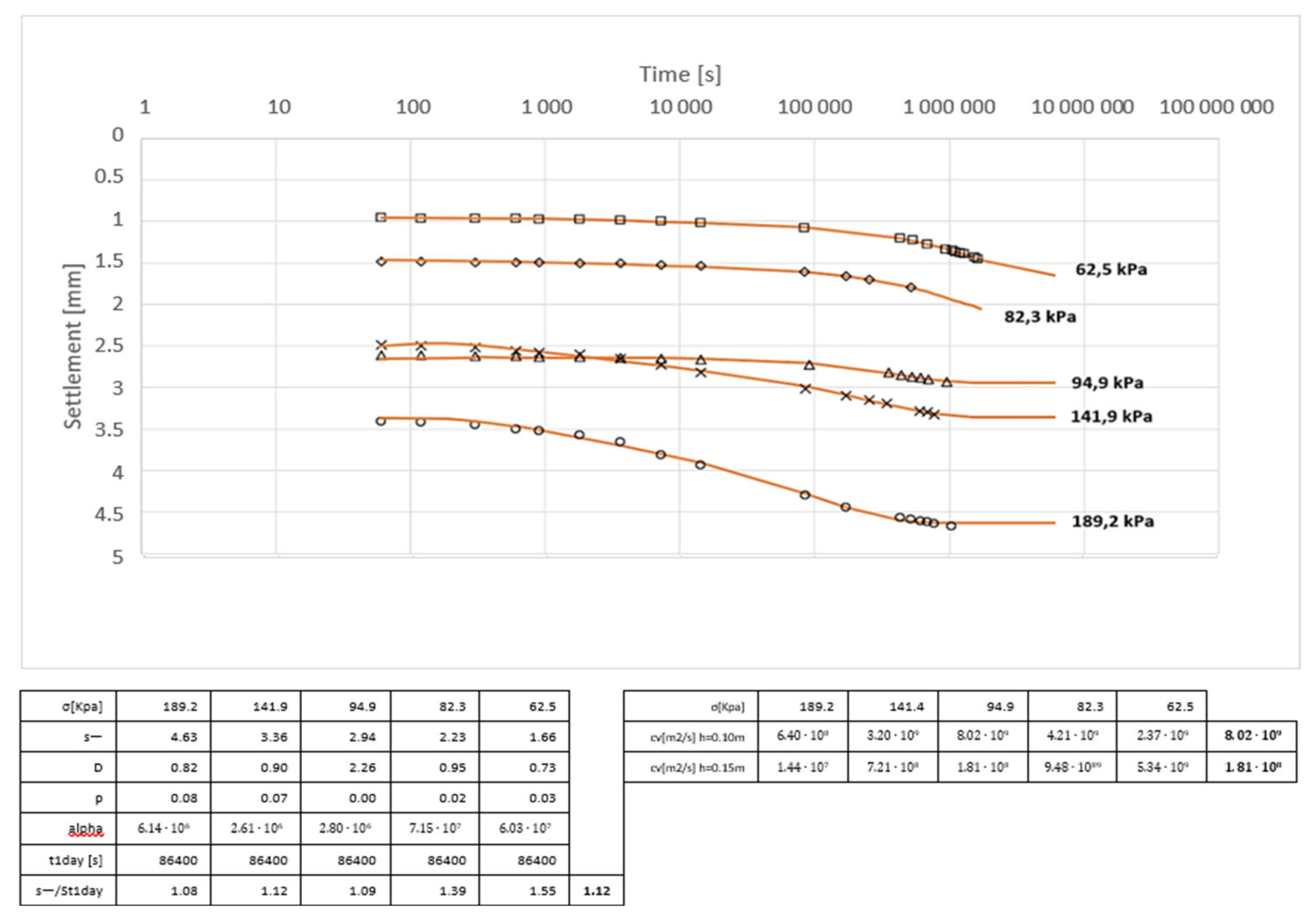
4. Consolidation Settlements
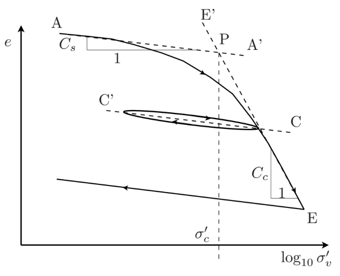
5. Preconsolidation Stress σ’c
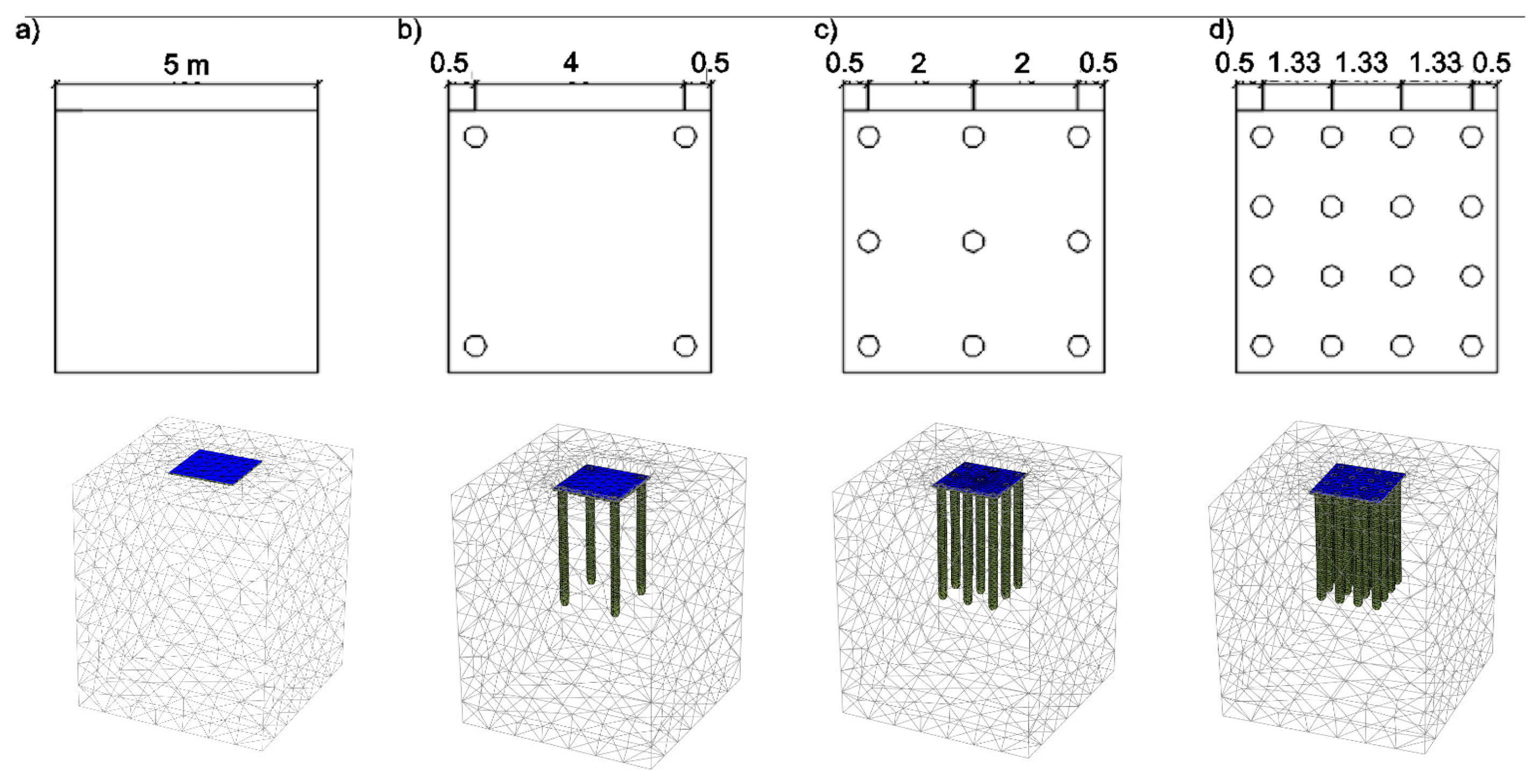
6. Numerical Analysis of Large-Dimensional Test Loads of Slab–Pile Foundations
6.1. Geometric Systems
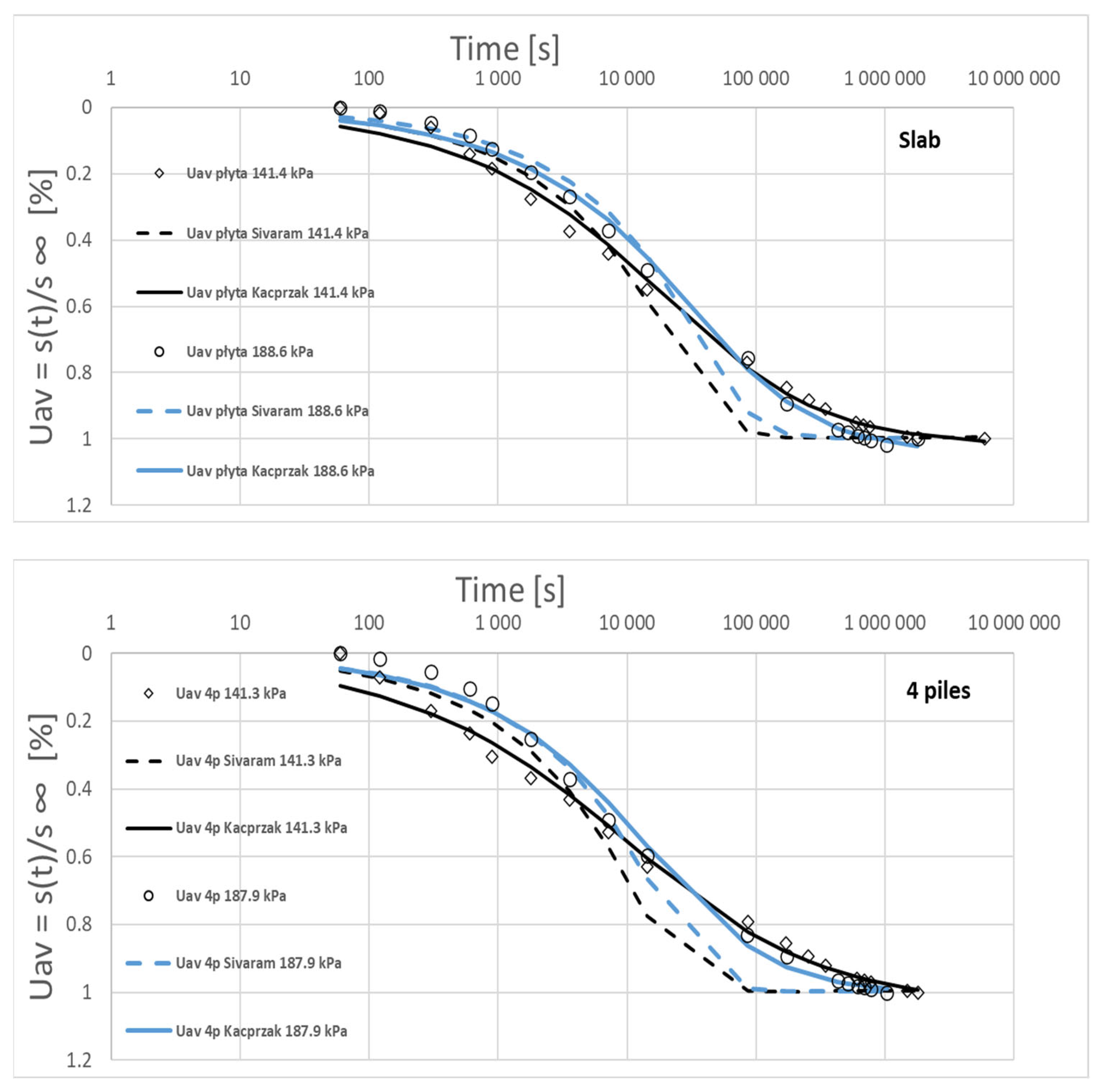
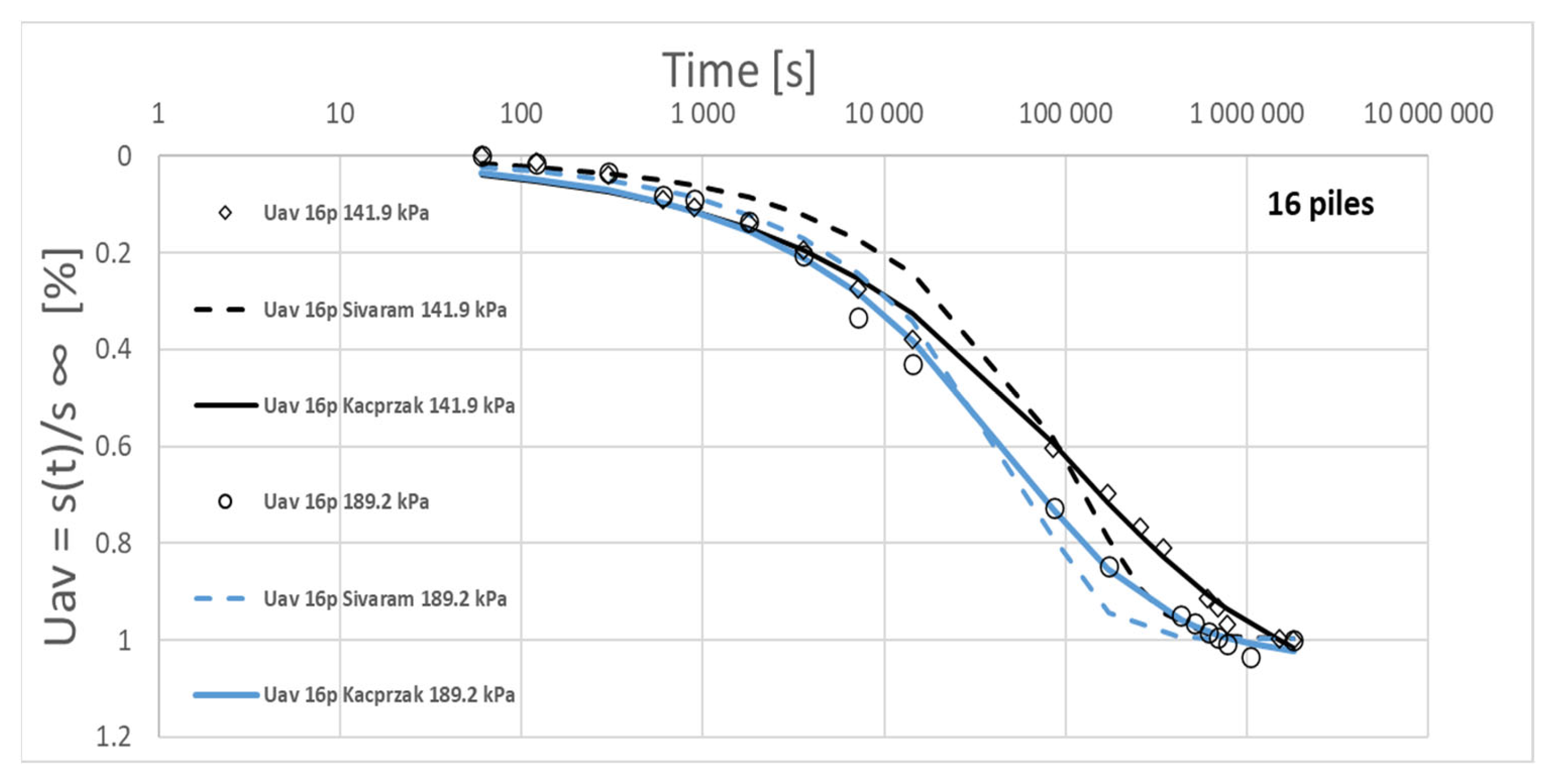
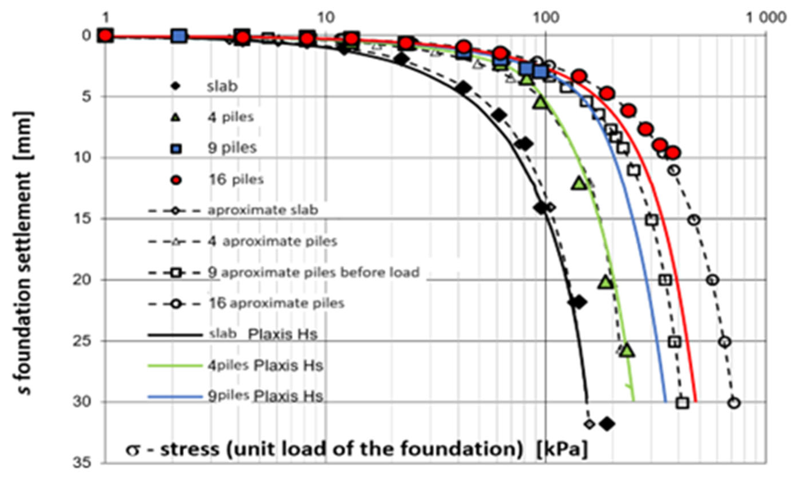
6.2. Comparison of Model Test Results with FEM Analysis Results
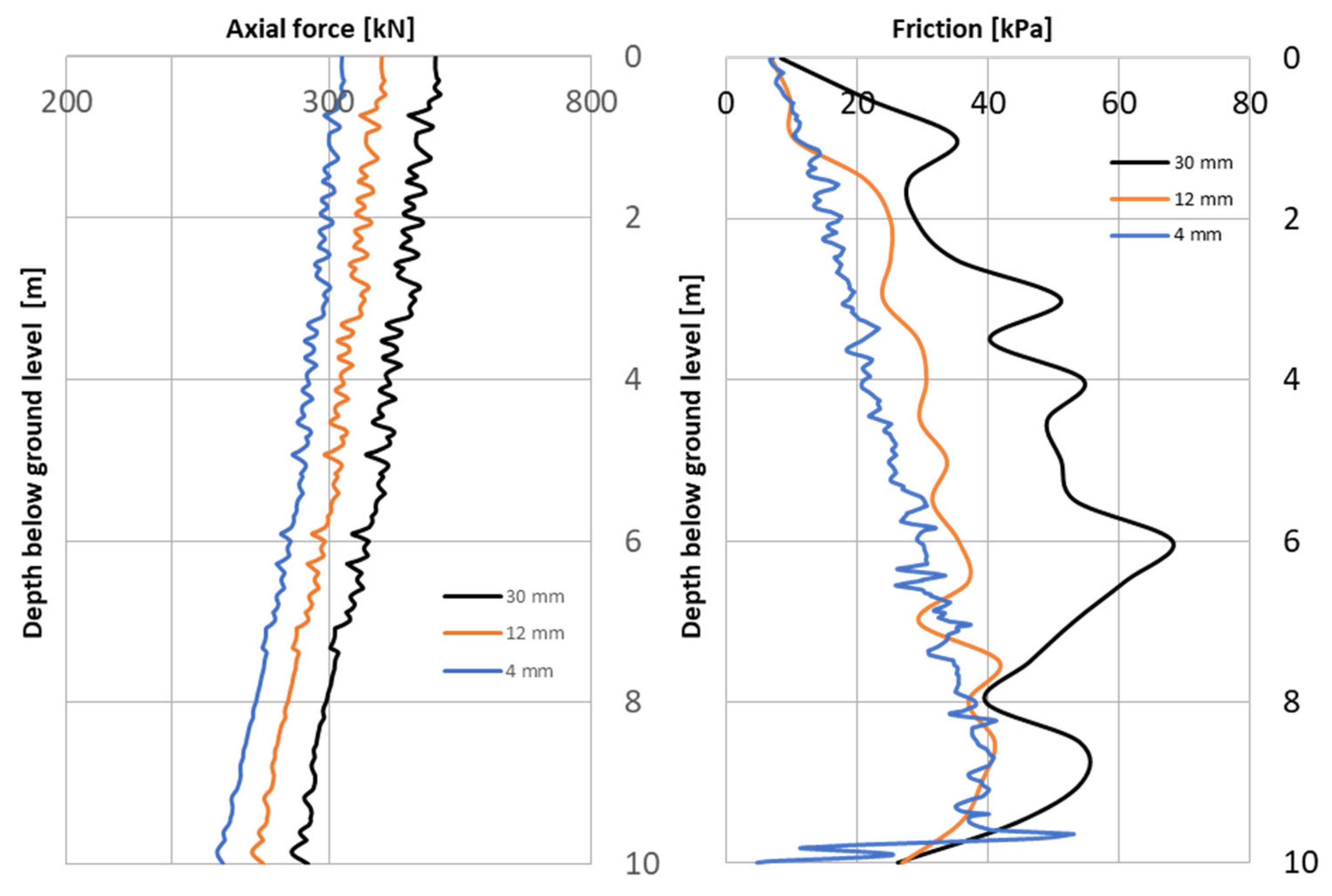
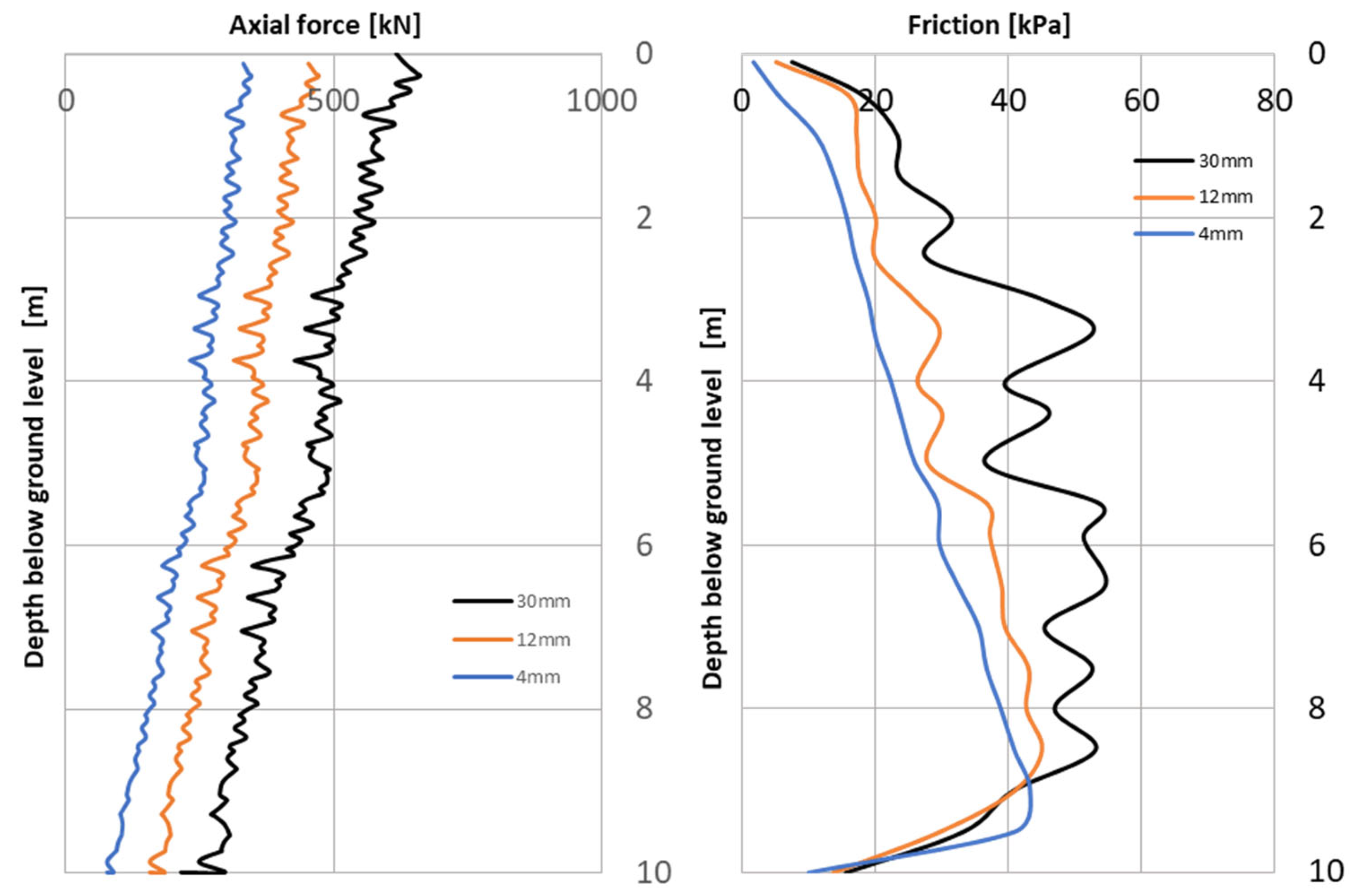
6.3. Analysis of Column Behavior Based on FEM Analysis
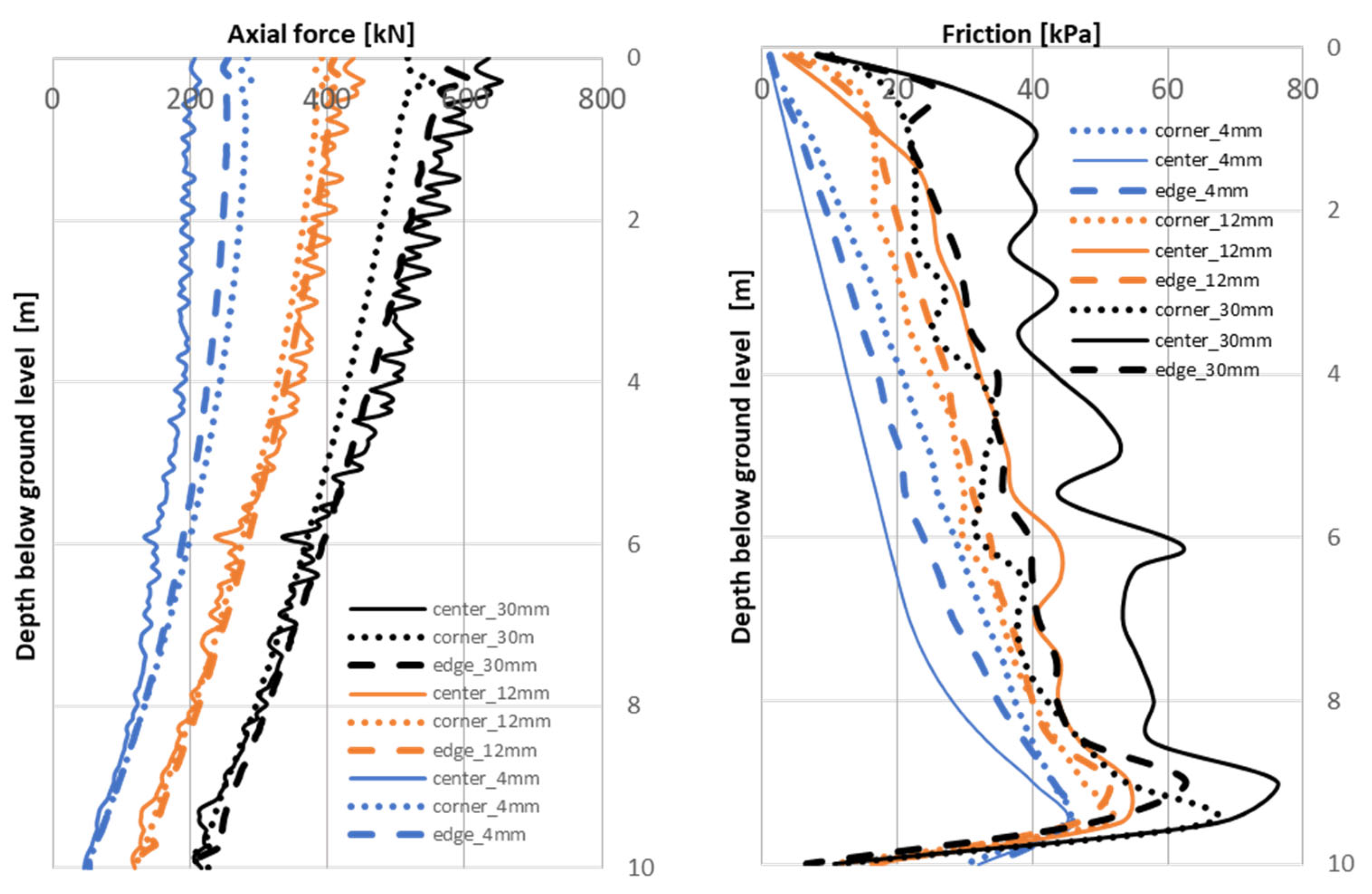
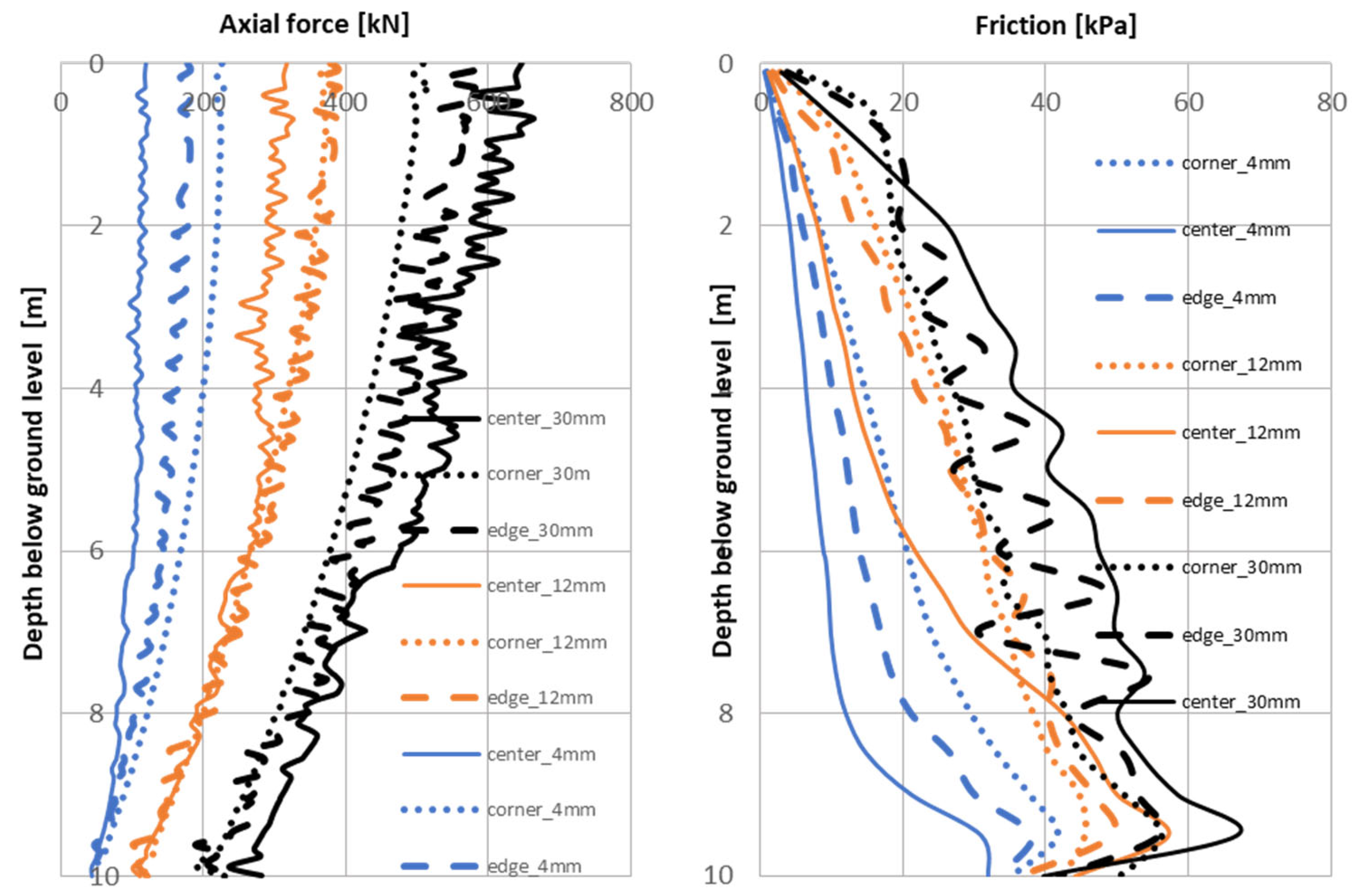
- The greater the settlement (increase in column head settlement from 4 mm to 30 mm), the greater the value of friction mobilized along the column (Figure 14, Figure 15, Figure 16 and Figure 17, figure on the right, a noticeable increase in friction—smallest values for blue, higher for orange, highest for black lines);
- By comparing the mobilization of friction on the shaft of the column (Figure 14, Figure 15, Figure 16 and Figure 17, figure on the right) for example for the central columns marked with a continuous blue line, we observe under the slab in pile–raft foundations a reduction in the mobilization of friction on the pile shaft; for example, for a depth of 2 m, the friction (kPa) decreases from 17.1 kPa—single column to 15.8 kPa—column in 4 pile–raft foundation, to 6.4 kPa—column in 9 pile–raft foundation, and finally to 5.88 kPa—column in 16 pile–raft foundation); we observe the so-called formation of a “dead zone” to a depth that depends on the spacing and mutual location of the piles, as well as the amount of settlement of the foundation;
- For the range of very small column head settlements (0.01D, blue line), for relative column spacing r/D = 3.3 (Figure 17, figure on the left) to r/D = 5 (Figure 16, figure on the left), the center columns (marked with a continuous line) mobilize less resistance than the edge columns (indicated by a dashed line), or the corner columns (indicated by a dotted line) working most effectively;
- For a range of small column head settlements (0.03D, orange line), for relative column spacing r/D = 3.3 (Figure 17, figure on the left), center columns (marked with a continuous line) mobilize less resistance than edge columns (indicated by a dashed line) or corner columns (indicated by a dotted line);
- For the range of small column head settlements (0.03D, orange line), for relative column spacings r/D = 5 (Figure 16, figure on the left), regardless of their location in the group, the columns mobilize similar resistance;
- For the range of large settlements of the column head (0.08D, black line), for the relative spacing of the columns r/D = 3.3 (Figure 17, figure on the left) to r/D=5 (Figure 16, figure on the left), the center columns (continuous line), due to the significant pressure of the slab, mobilize the greatest resistance; the corner columns (dotted line) work least effectively.
7. Conclusions
Author Contributions
Funding
Data Availability Statement
Conflicts of Interest
References
- PN-81/B-03020; Building Soils. Direct Foundation of Structures. Static Calculations and Design. Polish Committee for Standardization: Warsaw, Poland, 2013.
- PN-EN 1997-1:2008; Eurocode 7—Geotechnical Design Part 1: General Principles. European Committee for Standardization: Brussels, Belgium, 2008.
- PN-EN 1997-2:2009; Eurocode 7—Geotechnical Design Part 2: Reconnaissance and Investigation of the Ground. European Committee for Standardization: Brussels, Belgium, 2009.
- Geotechnics. Design of direct foundations. Amendment of PN-81/B-03020. Harmonization of Polish Geotechnical Standards with the System of European Standards, Mrągowo, Poland, November 2000.
- Combarieu, O. Calcul D’une Fondation Mixte Semellepieux Sous Chargé Verticale Centrée; Ministere de l’Equipement et Logement; Note d’information technique; Laboratoire Central des Ponts et Chaussees (LPCP): Paris, France, 1988; p. 16. [Google Scholar]
- Lavoie, F.L.; Kobelnik, M.; Valentin, C.A.; da Silva Tirelli, É.F.; de Lurdes Lopes, M.; Lins da Silva, J. Environmental Protection with HDPE Geomembranes in Mining Facility Constructions. Constr. Mater. 2021, 1, 122–133. [Google Scholar] [CrossRef]
- Farrag, S.; Gucunski, N. Evaluation of DSSI Effects on the Dynamic Response of Bridges to Traffic Loads. Constr. Mater. 2023, 3, 354–376. [Google Scholar] [CrossRef]
- Khalid, R.A.; Ahmad, N.; Arshid, M.U.; Zaidi, S.B.; Maqsood, T.; Hamid, A. Performance evaluation of weak subgrade soil under increased surcharge weight. Constr. Build. Mater. 2022, 318, 126131. [Google Scholar] [CrossRef]
- Wang, F.; Shao, J.; Li, W.; Wang, Y.; Wang, L.; Liu, H. Study on the Effect of Pile Foundation Reinforcement of Embankment on Slope of Soft Soil. Sustainability 2022, 14, 14359. [Google Scholar] [CrossRef]
- Borel, S. Comportement et Dimensionnement des Fondations Mixtes, Etudes et Recherches des Laboratoires des Ponts et Chaussées: Géotechnique et Risques Naturels, Études et Recherches des Laboratoires des Ponts et Chaussées; Série Géotechnique; Laboratoire Central des Ponts et Chaussees: Paris, France, 2001; ISBN 2-7208-2017-2. [Google Scholar]
- DIN 1054:2010-12; Baugrund—Sicherheitsnachweise im Erd- und Grundbau—Ergänzende Regelungen zu DIN EN 1997-1. Deutsches Institut für Normung: Berlin, Germany, 2010.
- Hanisch, J.; Katzenbach, R.; Konig, G. Kombinierte Pfahl-Plattengründungen; Ernst and Sohn: Berlin, Germany, 2002. [Google Scholar]
- Katzenbach, R.; Choudhury, D.; Ramm, H. ISSMGE Technical Committee Annual Report, Annexure 1: International CPRF Guideline, 24 May 2012; ISSMGE: London, UK, 2012. [Google Scholar]
- Katzenbach, R.; Choudhury, D. ISSMGE Combined Pile-Raft Foundation Guideline; Technische Universität Darmstadt, Institute and Laboratory of Geotechnics: Darmstadt, Germany, 2013. [Google Scholar]
- ASIRI. ASIRI National Project: Recommendations for the Design, Execution and Control of Rigid Inclusion Ground Improvements; IREX I Press de Ponts: Paris, France, 2013. [Google Scholar]
- Katzenbach, R.; Moormann, C. Recommendations for the design and construction of piled rafts. In Proceeding of the 15th International Conference on Soil Mechanics and Foundation Engineering, Istanbul, Turkey, 27–31 August 2001. [Google Scholar]
- Lindh, P.; Lemenkova, P. Geotechnical Properties of Soil Stabilized with Blended Binders for Sustainable Road Base Applications. Constr. Mater. 2023, 3, 110–126. [Google Scholar] [CrossRef]
- Wysokiński, L.; Kotlicki, W.; Godlewski, T. Projektowanie Geotechniczne Według Eurokodu 7, Poradnik; Instytut Techniki Budowlanej: Warsaw, Poland, 2011; p. 289. [Google Scholar]
- Kacprzak, G.; Zbiciak, A.; Józefiak, K.; Nowak, P.; Frydrych, M. One-Dimensional Computational Model of Gyttja Clay for Settlement Prediction. Sustainability 2023, 15, 1759. [Google Scholar] [CrossRef]
- Poulos, H.G. Piled raft foundations: Design and applications. Géotechnique 2001, 51, 95–113. [Google Scholar] [CrossRef]
- Sivaram, B.; Swamee, P. A Computational Method for Consolidation Coefficient. Soils Found. Tokyo 1977, 17, 48–52. [Google Scholar] [CrossRef] [PubMed]
- Lambe, T.W.; Whitman, R.V. Mechanika Gruntów,Tom I i II; Arkady: Warsaw, Poland, 1976–1977. [Google Scholar]
- Reuil, O.; Randolph, M.F. Optimised Design of Combined Pile Raft Foundations. In Combined Pile Raft Foundations; Darmstadt Geotechnics no. 18; Katzenbach, R., Ed.; Institute and Laboratory of Geotechnics: Darmstadt, Germany, 2009; pp. 149–169. [Google Scholar]
- Godlewski, T.; Fudali, J.; Saloni, J. Wzmocnienie podłoża budynku metodą kolumn betonowych (CMC). Inżynieria I Bud. 2007, 12, 661–663. [Google Scholar]
- Godlewski, T.; Wszędyrówny-Nast, M. Wybór metody posadowienia na przykładzie dużego budynku na słabym podłożu. In Proceedings of the X Konferencja Naukowo Techniczna Problemy Rzeczoznawstwa Budowlanego, Warsaw, Poland, 24 April 2008. 22 Z. [Google Scholar]
- Jiang, X.; Gabrielson, J.; Titi, H.; Huang, B.; Bai, Y.; Polaczyk, P.; Hu, W.; Zhang, M.; Xiao, R. Field investigation and numerical analysis of an inverted pavement system in Tennessee, USA. Constr. Build. Mater. 2022, 35, 100759. [Google Scholar] [CrossRef]
- Tang, R.; Wang, Y.; Zhang, W.; Jiao, Y. Load-Bearing Performance and Safety Assessment of Grid Pile Foundation. Sustainability 2022, 14, 9477. [Google Scholar] [CrossRef]
- Zhang, Y.; Deng, Z.; Chen, P.; Luo, H.; Zhang, R.; Yu, C.; Zhan, C. Experimental and Numerical Analysis of Pile–Rock Inter-action Characteristics of Steel Pipe Piles Penetrating into Coral Reef Limestone. Sustainability 2022, 14, 13761. [Google Scholar] [CrossRef]
- Plati, C.; Tsakoumaki, M. A Critical Comparison of Correlations for Rapid Estimation of Subgrade Stiffness in Pavement Design and Construction. Constr. Mater. 2023, 3, 127–142. [Google Scholar] [CrossRef]


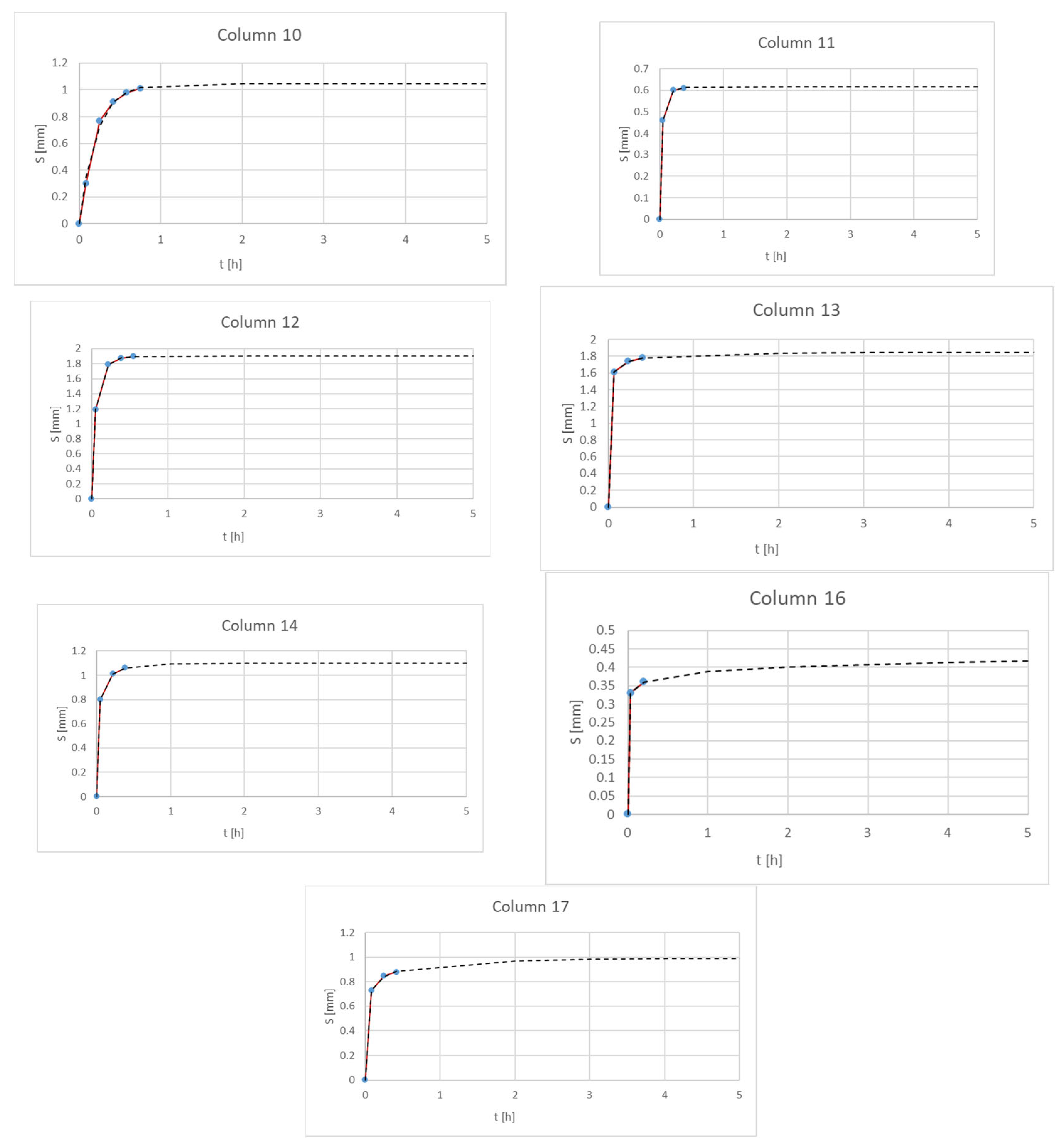
| Column | 1 | 3 | 4 | 10 | 12 | 13 | 14 | 17 |
|---|---|---|---|---|---|---|---|---|
| s∞ | 2.73 | 1.23 | 1.99 | 1.05 | 1.90 | 1.84 | 1.10 | 1.00 |
| De | 3.01 | 5.00 | 1.39 | 1.00 × –11 | 4.99E | 3.80 | 3.65 | 2.85 |
| p | 7.39 × 10⁻¹ | 4.19 × 10⁻¹ | 1.00 × 10⁻³ | 1.05 × 101 | 6.19 × 10⁻¹ | 2.34 × 10⁻¹ | 3.72 × 10⁻¹ | 3.10 × 10⁻¹ |
| α | 1.00 × 10⁻⁶ | 1.34 | 1.41 | 4.82 | 4.03 | 8.19 × 10⁻¹ | 2.10 | 1.00 × 10⁻⁶ |
| Column | 7 | 8 | 9 | 11 | 16 |
|---|---|---|---|---|---|
| s∞ | 5.32 × 10⁻¹ | 7.10 × 10⁻¹ | 1.01 | 6.17 × 10⁻¹ | 7.77 × 10⁻¹ |
| De | 4.10 × 10⁻¹ | 2.68 | 5.56 × 10⁻¹ | 5.00 | 6.92 × 10⁻¹ |
| p | 1.00 × 10⁻³ | 3.11 × 10⁻¹ | 8.72 × 10⁻² | 4.99 × 10⁻¹ | 6.61 × 10⁻² |
| α | 1.82 | 1.00 × 10⁻⁶ | 2.90 × 10⁻¹ | 5.00 | 4.80 × 10⁻⁵ |
| Column | 1 | 3 | 4 | 7 | 8 | 9 | 10 | 11 | 12 | 13 | 14 | 16 | 17 |
|---|---|---|---|---|---|---|---|---|---|---|---|---|---|
| se | 0.08 | 0.03 | 0.24 | 0.13 | 0.10 | 0.54 | 0.04 | 0.01 | 0.00 | 0.06 | 0.04 | 0.42 | 0.12 |
| sc | 2.73 | 1.23 | 1.99 | 0.53 | 0.71 | 1.01 | 1.05 | 0.62 | 1.90 | 1.84 | 1.10 | 0.78 | 1.00 |
| se/sc | 0.03 | 0.02 | 0.12 | 0.25 | 0.14 | 0.53 | 0.04 | 0.01 | 0.00 | 0.03 | 0.03 | 0.54 | 0.12 |
| Slab | Slab + 4 Piles | Slab + 16 Piles | |||
|---|---|---|---|---|---|
| 142 kPa | 142 kPa | 142 kPa | |||
| A | 0.434 | A | 0.396 | A | 0.387 |
| B | 0.793 | B | 0.649 | B | 0.970 |
| C | 0.543 | C | 0.601 | C | 0.366 |
| 189 kPa | 189 kPa | 189 kPa | |||
| A | 0.456 | A | 0.494 | A | 0.441 |
| B | 1.117 | B | 1.014 | B | 1.320 |
| C | 0.399 | C | 0.487 | C | 0.325 |
| γ (kN/m3) | Material | E (kN/m2) | ν | Thickness (m) |
|---|---|---|---|---|
| 0 | Linear, isotropic | 30 × 106 | 0.2 | 0.3 |
| γ (kN/m3) | Conditions | einitial | E50ref (kN/m2) | Eedoref (kN/m2) | Eurref (kN/m2) | pref |
| 15 | drained | 0.5 | 67.2 × 10³ | 67.2 × 10³ | 134.4 × 10³ | 100 |
| νur | c (kN/m2) | ϕ (ο) | ψ (ο) | K0NC | Interface | Rf |
| 0.3 | 4 | 18.5 | 0 | 0.68 | 0.67 | 0.9 |
| γ (kN/m3) | Material | Type | E (kN/m2) | ν | Interface | Diameter (m) |
|---|---|---|---|---|---|---|
| 24 | Linear isotropic | Poreless | 30 × 106 | 0.2 | 1.0 | 0.4 |
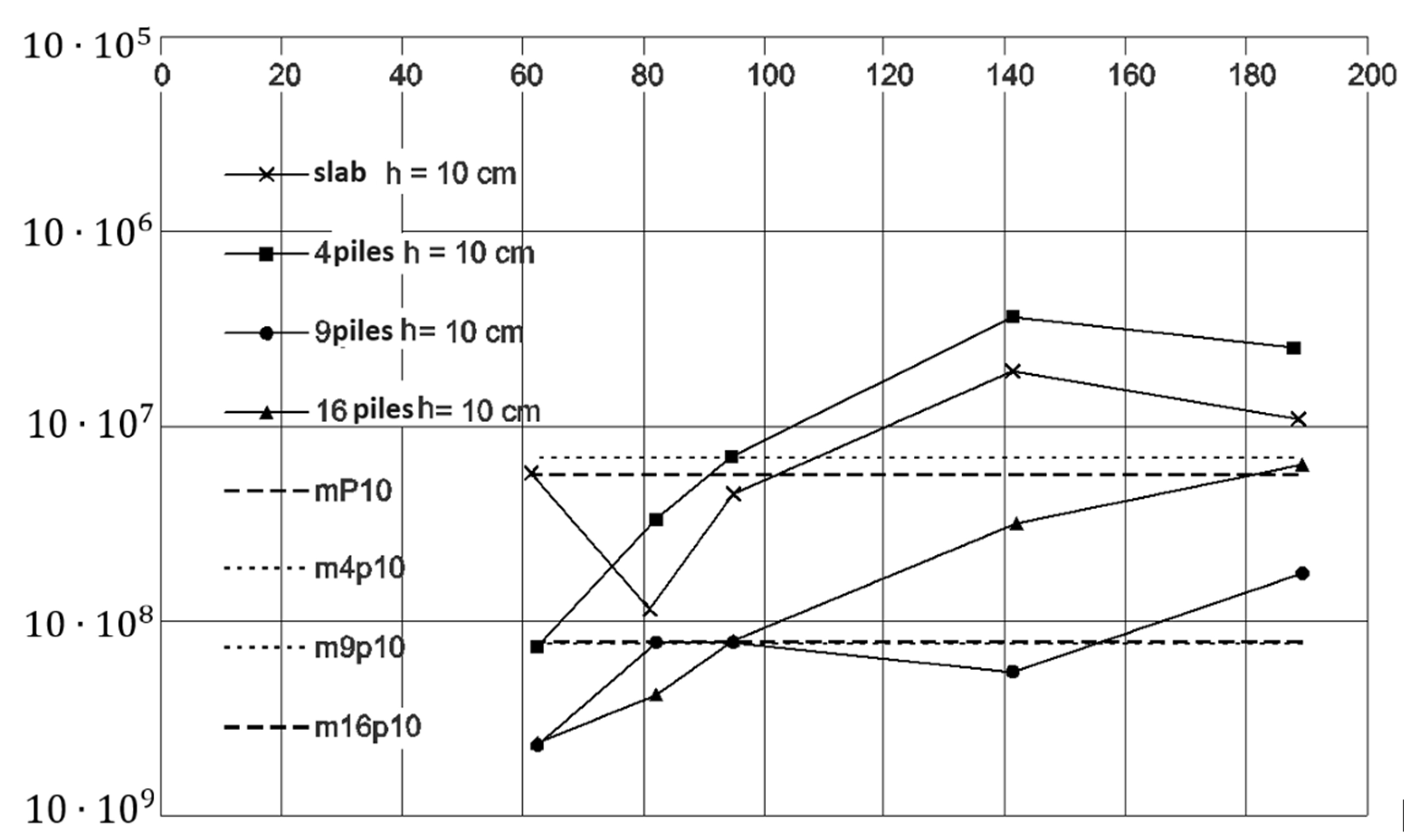
| Type CPRF | Approximate Load Range (kPa) | Approximating Function | Coefficient of Determination R2 |
|---|---|---|---|
| slab | 119–154 | y = 43.795ln(x) − 191.43 | 0.985 |
| slab + 4 piles | 180–250 | y = 44.83ln(x) − 217.92 | 0.962 |
| slab + 9 piles | 254–351 | y = 44.975ln(x) − 234.26 | 0.992 |
| slab + 16 piles | 343–481 | y = 44.435ln(x) − 245.27 | 0.990 |
Disclaimer/Publisher’s Note: The statements, opinions and data contained in all publications are solely those of the individual author(s) and contributor(s) and not of MDPI and/or the editor(s). MDPI and/or the editor(s) disclaim responsibility for any injury to people or property resulting from any ideas, methods, instructions or products referred to in the content. |
© 2023 by the authors. Licensee MDPI, Basel, Switzerland. This article is an open access article distributed under the terms and conditions of the Creative Commons Attribution (CC BY) license (https://creativecommons.org/licenses/by/4.0/).
Share and Cite
Kacprzak, G.; Frydrych, M. Soil Consolidation Analysis in the Context of Intermediate Foundation as a New Material Perspective in the Calibration of Numerical–Material Models. Constr. Mater. 2023, 3, 414-433. https://doi.org/10.3390/constrmater3040027
Kacprzak G, Frydrych M. Soil Consolidation Analysis in the Context of Intermediate Foundation as a New Material Perspective in the Calibration of Numerical–Material Models. Construction Materials. 2023; 3(4):414-433. https://doi.org/10.3390/constrmater3040027
Chicago/Turabian StyleKacprzak, Grzegorz, and Mateusz Frydrych. 2023. "Soil Consolidation Analysis in the Context of Intermediate Foundation as a New Material Perspective in the Calibration of Numerical–Material Models" Construction Materials 3, no. 4: 414-433. https://doi.org/10.3390/constrmater3040027
APA StyleKacprzak, G., & Frydrych, M. (2023). Soil Consolidation Analysis in the Context of Intermediate Foundation as a New Material Perspective in the Calibration of Numerical–Material Models. Construction Materials, 3(4), 414-433. https://doi.org/10.3390/constrmater3040027