Unified Evaluation of Slope Displacements Using Energy-Based Newmark Method for Arbitrary Earthquake Motions

Abstract

Slope displacements (δ) have been shown to correlate uniquely with the earthquake energy (E_eq) contributing to slope sliding, regardless of input motion characteristics. Based on this principle, this study applies the Energy-Based Newmark Method to infinitely long slopes subjected to ten diverse earthquake records with stepwise scaled amplitudes. As the earthquake wave energy (Eᵤ) increases, the energy ratio (E_eq/Eᵤ) exhibits a distinct peak followed by a monotonic decrease. The peak values and corresponding Eᵤ levels strongly depend on the predominant frequencies (f_p) of the motions, consistent with results from harmonic wave analyses. A unified design diagram is developed to correlate E_eq/Eᵤ with Eᵤ, incorporating f_p and slope parameters. Since both Eᵤ and f_p can be determined from design motions or empirically predicted using earthquake magnitudes and source distances, the slope displacement δ can be directly obtained from the diagram, eliminating the need for time-domain numerical simulations used in the conventional Newmark approaches. This method is recommended to conduct seismic zonation and hazard mapping in mountainous and hilly regions for regional authorities and infrastructure planners.

1. Introduction

Earthquake-induced slope displacements are commonly evaluated in engineering practice using the Newmark slope model, originally proposed by Newmark [1]. In this model, a rigid soil block above a predefined potential slip plane is subjected to a design acceleration motion, and the driving force is compared with the corresponding resistance along the slip plane (Sarma [2], Crespellani et al. [3]).

Alternatively, local accelerations within a deformable soil slope obtained from dynamic response analyses of decoupled finite element methods (FEM) that account for seismic amplifications are used to calculate the global driving force. This force is then compared with the shear resistance along the slip plane (Makdisi & Seed [4], Watanabe et al. [5]). If the safety factor (defined as resistance divided by driving force) falls below unity during a given time interval of an earthquake motion, the sliding displacement is computed using the Newmark slope sliding algorithm (e.g., Kokusho [6]). Furthermore, while seismic amplification and sliding displacement are often evaluated separately in decoupled analyses, coupled evaluations have also been developed and applied to case studies (Kramer & Smith [7], Rathje & Bray [8]).

While the Newmark method was originally based on straight slip planes, circular slip planes are frequently used in current civil engineering practice, in which the driving moment about the circle center is compared to the resisting moment along the circular plane. Both of them share the basic equation of force equilibrium, though resulting displacements are typically limited to a few meters in the circular planes.

In contrast, strong earthquakes have repeatedly triggered long-distance failures in natural slopes, causing catastrophic damage. Massive debris flows have traveled considerable distances, impacting residential areas, infrastructures, and river flows. To evaluate such devastating failures, Kokusho and Ishizawa [9] developed an energy-based approach using shaking table model tests, replacing the principle of force equilibrium with that of energy balance. A key finding of this approach was that slope sliding displacements δ are uniquely formulated with earthquake wave energies E_eq directed toward slope sliding, regardless of the input motion characteristics. Numerous case histories of slope failures during recent earthquakes have been back-analyzed using this formula by Kokusho et al. [10,11] to understand failure mechanisms and quantify mobilized friction coefficients.

Building on the energy balance concept, the “Energy-Based Newmark Method” was developed by Kokusho et al. [12]. This method couples the Newmark-type slope model with an underlying horizontal layer where SH waves propagate to directly evaluate slope displacements δ from upward wave energy E_u. The application of the method has been limited so far within harmonic motions and cannot be extended to irregular earthquake waves useful in practical design.

In this study, widely diverse ten irregular earthquake motions recorded during recent destructive events in Japan are applied with stepwise increasing amplitudes to an infinitely long slope to calculate the earthquake energy for slope sliding E_eq from the input wave energies E_u. The relationship between E_eq and E_u is then modified to construct a unified diagram, enabling E_eq to be estimated from E_u using wave and slope parameters for arbitrary earthquake motions. This allows slope displacements δ to be determined directly from E_eq based on the energy balance without resorting to numerical analyses by the conventional Newmark method.

2. Energy Principles for Slope Sliding

The energy balance governing earthquake-induced slope failures was first formulated by Kokusho and Kabasawa [13] as

$$E_{gr}+E_{eq}=E_{dp}+E_k$$

(1)

where E_gr = gravitational energy variation due to slope sliding, E_eq = earthquake energy contributing to sliding, E_dp = energy dissipated in the slope during sliding, and E_k = kinetic energy of the slope during sliding. All energies are defined per unit horizontal area of the slip plane. If the energy balance is considered before and after sliding (i.e., E_k = 0), Equation (1) simplifies to

$$E_{gr}+E_{eq}=E_{dp}$$

(2)

In a Newmark-type sliding block model (Figure 1a), with friction angle $\varphi$, slope angle $\theta$, and residual horizontal displacement δ, the gravitational and dissipated energies can be expressed [9] as

$$E_{gr}=\rho gD\delta \tan \theta$$

(3)

$$E_{dp}=\rho gD\delta \tan \varphi \left(1+{\tan }^2\theta \right)/(1+\tan \theta \tan \varphi )$$

(4)

where ρ = density of the sliding block, g = acceleration of gravity, and D = thickness of the sliding block. Substituting into Equation (2), the earthquake energy contributing to slope sliding becomes

$$E_{eq}=E_{dp}-E_{gr}=\rho gD\delta \tan \left(\varphi -\theta \right)$$

(5)

Thus, the residual displacement δ can be expressed directly from the energy balance:

$$\delta =E_{eq}/\left[\rho gD\tan \left(\varphi -\theta \right)\right]$$

(6)

which is central to the energy-based approach.

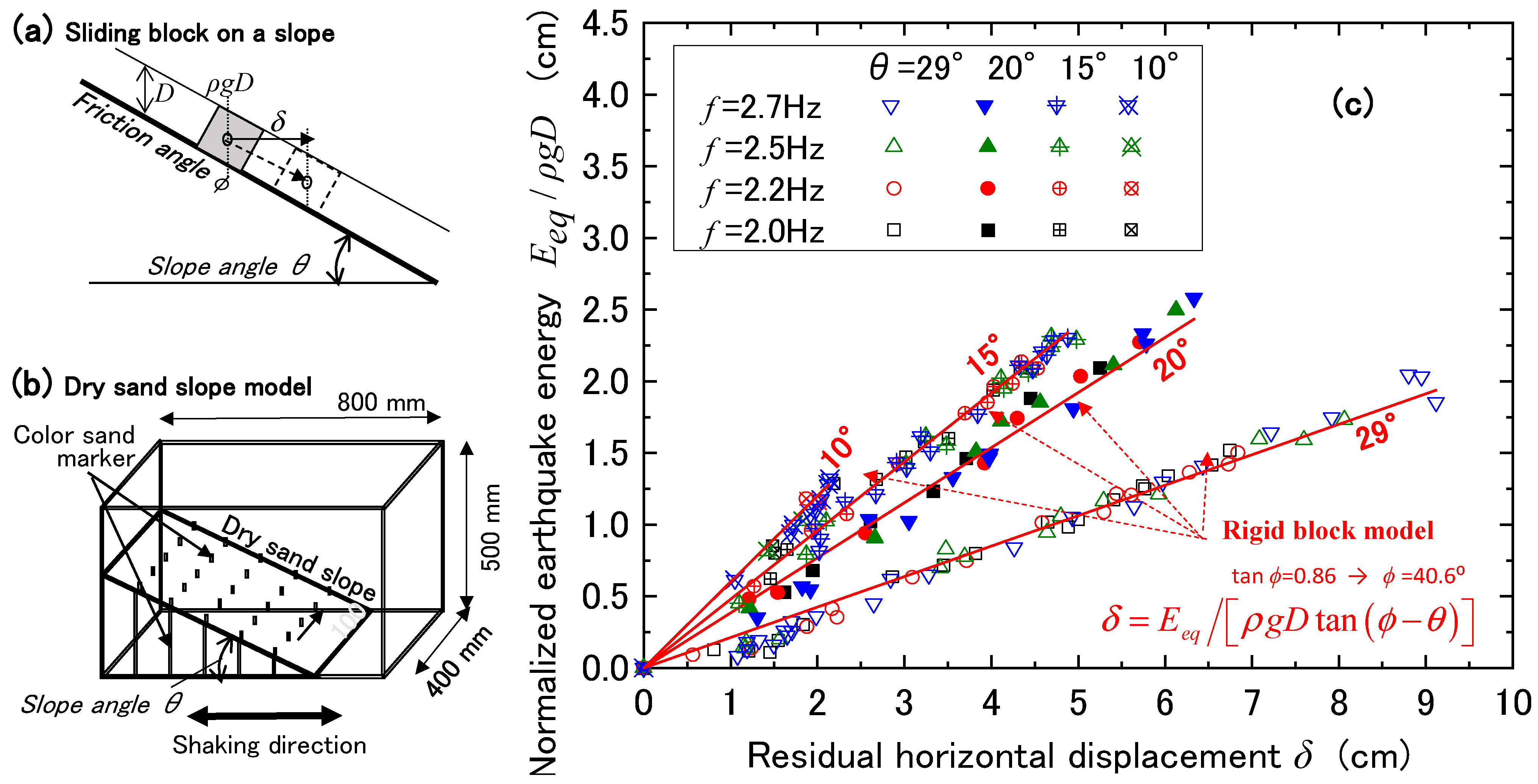
This equation was validated through shaking table tests (Figure 1b), in which dry sand slopes of varying slope angles were subjected to sinusoidal vibrations of different frequencies. Detailed descriptions of the test setup, energy measurements, and displacement evaluations are provided by [9]. In Figure 1c, normalized earthquake energies E_eq/ρgD are plotted against average slope displacements δ for slope angles of θ = 29°, 20°, 15°, and 10°. These test results are compared with straight lines derived from Equation (6), using an adjusted friction angle of $\varphi$ = 40.6°. Remarkably, the simple energy theory of a rigid block on a straight slope (Figure 1a) reproduces the observed displacements of sand slopes across all slope angles and input frequencies, provided that a suitable friction angle $\varphi$ is prescribed. This suggests that realistic failure modes, including continuous shear deformation, can be effectively captured by the energy-based approach employing the rigid slip plane.

The effectiveness of this approach was further demonstrated by applying Equation (6) to numerous case history slope failures during strong earthquakes in Japan. These back-analyses enabled estimation of mobilized friction angles and provided insights into the actual failure mechanisms [10,11]. It is worth noting that the Newmark slope model shares the same fundamental mechanism as the energy-based model in Figure 1a, assuming a rigid slip plane. Therefore, the Newmark model, when integrated with energy principles and appropriate friction coefficients, may serve as a practical tool for evaluating slope displacements in realistic shear failure modes.

3. Outline of Energy-Based Newmark Method (EBNM)

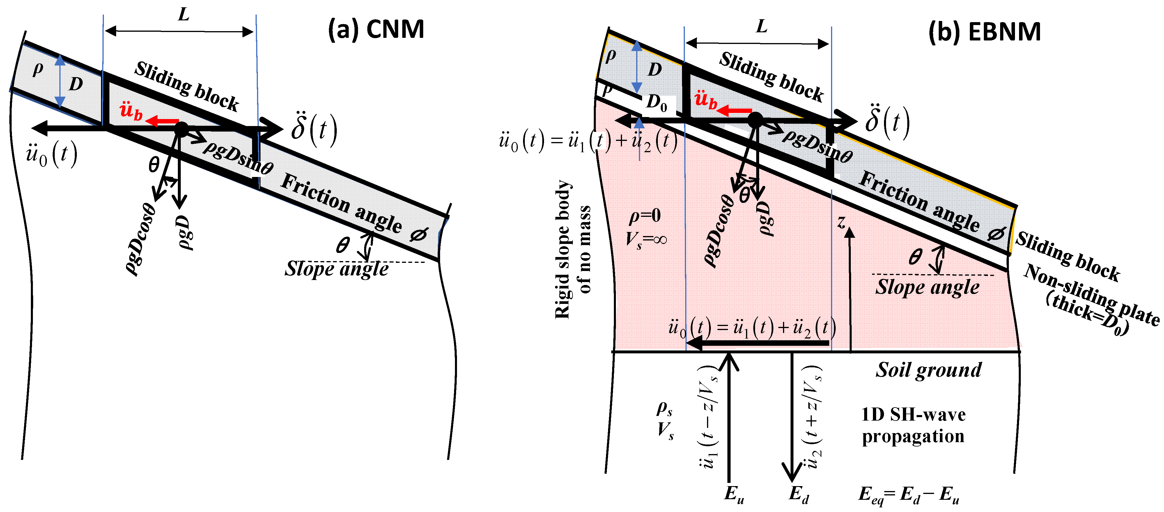
In Figure 2a, the conventional Newmark model (CNM) is illustrated as an infinitely long rigid slope of friction angle $\varphi$ and slope angle $\theta$ overlain by a sliding block of vertical thickness D and density ρ. Herein, the friction coefficient of the slope is represented solely as $\tan \varphi$ using the friction angle $\varphi$ to make the following analysis simpler, where the effect of cohesion c may be considered implicitly by reevaluating $\varphi$ as ${\tan }^{-1}\left(\tan \varphi +c/{\sigma }_v\right)\to \varphi$ assuming constant overburden stress ${\sigma }_v$.

If the acceleration working on the slope ${\ddot{u}}_0$ exceeds the yield acceleration in the CNM, $g\tan \left(\varphi -\theta \right)$, in the downslope direction;

$${\ddot{u}}_0-g\tan \left(\varphi -\theta \right)>0$$

(7)

then, the block starts sliding with the relative acceleration $\ddot{\delta }$ as

$$\ddot{\delta }=\left[{\ddot{u}}_0-g\tan \left(\varphi -\theta \right)\right]\cos \left(\varphi -\theta \right){\displaystyle \frac{\cos \theta }{\cos \varphi }}$$

(8)

In Figure 2b, the Energy-Based Newmark Method (EBNM) is illustrated, wherein the most pronounced difference from the CNM is how to give an input acceleration to the slope. A virtual slope body is brought in as shaded in the figure beneath the sliding block in contact with a horizontal ground underneath, where the SH-wave input motion is coming up. The horizontal wave displacement $u\left(t,z\right)$ in the soil layer of S-wave velocity V_s for time t and vertical coordinate z (upward plus) can be written as

$$u\left(t,z\right)=u_1\left(t-z/V_s\right)+u_2\left(t+z/V_s\right)$$

(9)

where u₁ and u₂ stand for horizontal displacements of upward and downward SH-waves, respectively. Hence, the acceleration at the top of the soil ground z = 0 is

$$\ddot{u}\left(t,0\right)\equiv {\ddot{u}}_0\left(t\right)={\ddot{u}}_1\left(t\right)+{\ddot{u}}_2\left(t\right)$$

(10)

This acceleration ${\ddot{u}}_0\left(t\right)$ transmits directly to the slope surface through the slope body, which is virtually of infinite rigidity and has no mass without any wave amplification, and vibrates the sliding block in the same way as in the CNM.

Needless, Figure 2b is not a rigorous model replicating the wave propagation in two-dimensional sloping ground but a simplification from an engineering point of view. However, it may be justified for practical purposes because the CNM in Figure 2a, too, seems to involve implicitly a similar simplification wherein horizontal ground acceleration is loaded directly on the sliding slope mass. Also note that local wave amplification due to slope geometry is not taken into account here. This is because higher frequency motions, which amplify in local slope geometries, may be neglected in calculating slope slide displacements, which are overwhelmingly dominated by lower frequency waves, as addressed later.

The model in Figure 2b is further modified so that a thin non-sliding plate (thickness D₀, density $\rho$) is inserted beneath the sliding plane of friction angle $\varphi$, and glued to the top of the virtual slope body for the purpose of stabilizing the numerical integration in a time-domain dynamic response analysis, as will be explained later.

It is readily understandable in Figure 2b that the energy E_eq dissipated in slope sliding can be equated with the difference between upward and downward energy, $E_u$ and $E_d$, respectively, as

$$E_{eq}=E_u-E_d$$

(11)

if the seismic energy is postulated to flow exclusively vertically by the SH-wave in the horizontal layer. Here, E_u and E_d are calculated from corresponding upward and downward velocity motions, ${\dot{u}}_1\left(t\right)$ and ${\dot{u}}_2\left(t\right)$, one-directionally propagating SH-waves, respectively, for time interval t = 0~T of a particular earthquake motion (e.g., Sarma [14]) as

$$\left.\begin{array}{c}{E}_u={\rho }_s{V}_s{\displaystyle {\int }_0^T\left|{\left[{\dot{u}}_1\left(t\right)\right]}^2\right|}dt\\ E_d={\rho }_s{V}_s{\displaystyle {\int }_0^T\left|{\left[{\dot{u}}_2\left(t\right)\right]}^2\right|}dt\end{array}\right\}$$

(12)

The force equilibrium of the slope model shown in Figure 2b can then be formulated [12] as

$$\rho D\left({\ddot{u}}_0-\ddot{\delta }\right)+\rho D_0{\ddot{u}}_0+{\rho }_s{V}_s^2{\left.{\displaystyle \frac{\partial u}{\partial z}}\right|}_{z=0}=0$$

(13)

where the first and second terms are the inertia force of the sliding block and the non-sliding plate, respectively. The third term is the seismic shear stress working at the bottom of the virtual slope body. Then it becomes

$$\left[\rho D\left({\ddot{u}}_1\left(t\right)+{\ddot{u}}_2\left(t\right)-\ddot{\delta }\left(t\right)\right)\right]+\left[\rho D_0\left({\ddot{u}}_1\left(t\right)+{\ddot{u}}_2\left(t\right)\right)\right]={\rho }_s{V}_s\left[{\dot{u}}_1\left(t\right)-{\dot{u}}_2\left(t\right)\right]$$

(14)

If the slope starts sliding due to increasing acceleration, Equation (14), coupled with Equations (7) and (8), is transformed to Equation (15) using constants A and B defined in Equation (16).

$$\rho D\left\{{\ddot{u}}_1\left(t\right)+{\ddot{u}}_2\left(t\right)-\left[{\ddot{u}}_1\left(t\right)+{\ddot{u}}_2\left(t\right)+B\right]A\right\}+\rho D_0\left({\ddot{u}}_1\left(t\right)+{\ddot{u}}_2\left(t\right)\right)={\rho }_s{V}_s\left[{\dot{u}}_1\left(t\right)-{\dot{u}}_2\left(t\right)\right]$$

(15)

$$\left.\begin{array}{l}\ddot{\delta }\left(t\right)=\left[{\ddot{u}}_1\left(t\right)+{\ddot{u}}_2\left(t\right)+B\right]A\\ A=\mathrm{co}\left(\varphi -\theta \right)\cos \theta /\cos \varphi \\ B=-g\tan \left(\varphi -\theta \right)\end{array}\right\}$$

(16)

Equations (15) and (16) are further simplified as Equations (17) and (18) by introducing another constant M as follows.

$$M\left[{\ddot{u}}_1\left(t\right)+{\ddot{u}}_2\left(t\right)\right]={\rho }_s{V}_s\left[{\dot{u}}_1\left(t\right)-{\dot{u}}_2\left(t\right)\right]+\rho DAB$$

(17)

$$M=\rho D\left[1-A+\left(D_0/D\right)\right]$$

(18)

Considering that A defined in Equation (16) takes 1.0~1.1 for plausible design values as $\varphi -\theta$ = 0~35° and $\varphi$ = 35° in ordinary slope problems, M is destined to be negative if D₀ = 0 (the non-sliding plate is absent). This is why the thin plate was added in the model to create the term including D₀ so that Equation (17) can be time-integrated using the Newmark β-method with stability (Kokusho et al. [12]). However, the thickness D₀ of the non-sliding plate, virtually introduced solely for the sake of numerical stability, should be as small as possible to avoid its unfavorable effect. D₀/D = 0.12 has been chosen in Equation (18) by trial calculations so that D₀ is as near to zero as possible and M is still positive.

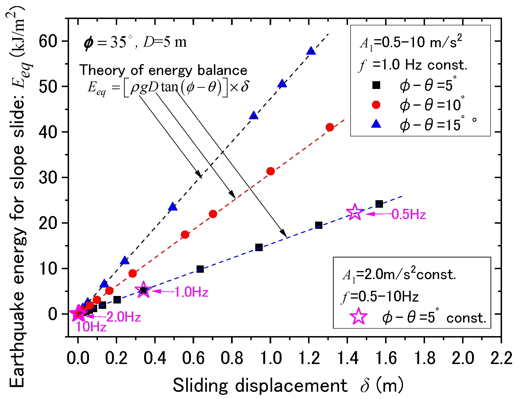
A series of finite difference calculations of the EBNM in Figure 2b have been conducted [12] for harmonic input motions utilizing Equations (17) and (18) for infinitely long slopes of $\varphi$ = 35°, $\varphi -\theta$ = 5, 10, 15°, ρ = ρ_s = 1.8 t/m³, V_s = 200 m/s, where harmonic motion f = 1.0 Hz is given with stepwise increasing amplitudes A₁. In Figure 3, the earthquake energies E_eq = E_u − E_d are plotted versus residual displacements δ of the sliding block. The calculated E_eq and δ are all evaluated as stationary values per one cycle. Three dashed lines in the chart representing the theoretical Equation (6) are in perfect agreement with the computed plots, indicating that the energy theory expressed in Equations (1) to (6) is replicated exactly by the Newmark calculation. Also note that the previously mentioned modification of the model with the additional non-sliding plate of D₀/D = 0.12 for numerical stability performs very well without any detrimental effects.

Furthermore, the star symbols in Figure 3, representing $\varphi -\theta$ = 5° and constant acceleration amplitude A₁ = 2.0 m/s² while the input frequency is varied f = 0.5~10 Hz stepwise, indicate that the energy theory in Equation (6) is universally applicable in evaluating slope displacements despite widely different input frequencies. In contrast, the acceleration A₁ cannot serve as a unique parameter, obviously, because the same acceleration 2.0 m/s² results in widely separated displacements δ due to the difference in frequency f. The above finding highlights how effective the energy concept is in evaluating slope displacements, as already demonstrated by a series of shaking table tests of model slopes [9], in contrast to the acceleration used in current practice.

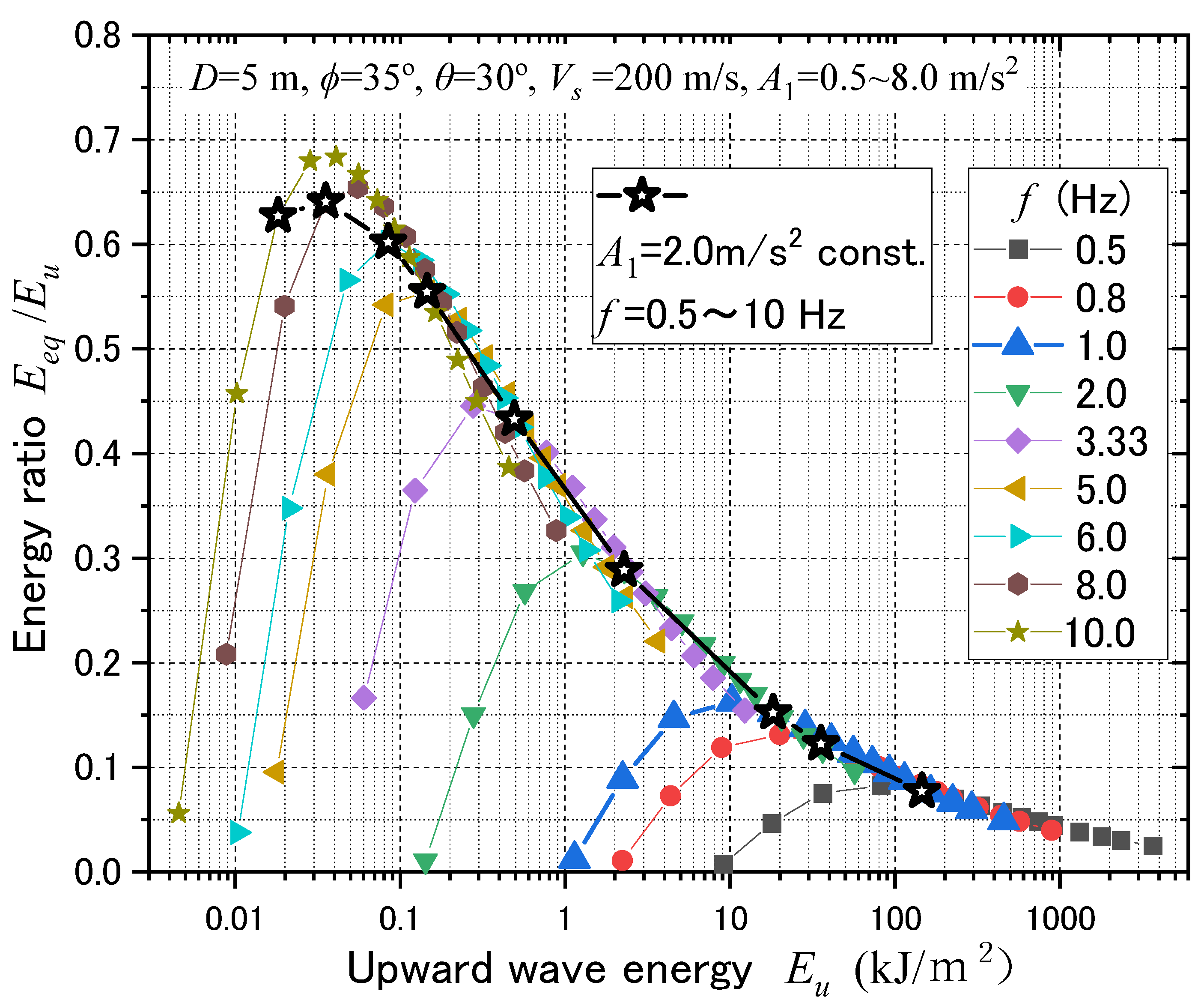
In Figure 4, the energy ratios E_eq/E_u calculated for harmonic waves of frequency f = 0.5 to 10 Hz are plotted on the vertical axis versus E_u in the horizontal log axis corresponding to stepwise-increasing wave amplitudes A₁ = 0.5~8.0 m/s². While E_eq simply increases with increasing E_u, E_eq/E_u shows a clear peak followed by a monotonic decline with increasing E_u, because the increment rate of E_eq to E_u tends to decrease in the midst of the E_eq~E_u relationship. Quite remarkably, the E_eq/E_u~E_u curves are very similar to each other, while the peak values (E_eq/E_u)_peak tend to be greater and occur at lower E_u as corresponding frequencies f of the harmonic motions are getting higher. This implies that there exists an optimum E_u depending on frequency f wherein the earthquake energy E_u is most efficiently directed to the energy E_eq for slope sliding.

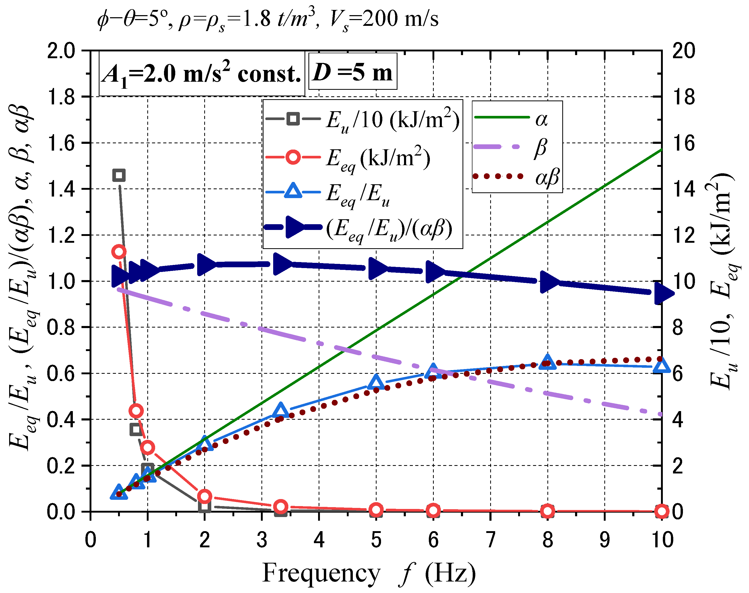
In Figure 5, the energy E_u, E_eq, and the ratio E_eq/E_u in a single cycle of a harmonic wave of constant acceleration amplitude A₁ = 2.0 m/s² are plotted against f = 0.5~10.0 Hz. E_u tends to decrease drastically in inverse proportion to the cube of f under a constant A_1, as implied in Equation (12). Accordingly, E_eq tends to decrease significantly with f compared to E_eq 100% at f = 1 Hz, down to 21% at f = 2 Hz, 6% at f = 3.3 Hz, and 2% at f = 5 Hz. Considering that the slide displacement δ is directly proportional to E_eq in Equation (6), high-frequency motions for f ≥ 3~4 Hz are almost ignorable in calculating slope slide displacements, as already stated above. In the same graph, the energy ratio E_eq/E_u calculated for A₁ = 2.0 m/s² constant is plotted with open triangular symbols against f. The same ratio E_eq/E_u is plotted versus E_u with star symbols in Figure 4 to compare with the E_eq/E_u versus E_u plots calculated for parametrically changing frequencies. This indicates that the values E_eq/E_u in Figure 5 are almost coincidental with the peak values (E_eq/E_u)_peak for f = 0.5~9.0 Hz in Figure 4. As for E_eq/E_u, a considerable surge of about 10 times is observed with increasing f from 0.5 to 10 Hz in Figure 5. However, if E_eq/E_u is normalized as (E_eq/E_u)/(αβ), it becomes almost f-insensitive within ±6% difference from the average over f = 0.5~10 Hz, as indicated with triangles connected with a thick curve. Here, constants α and β are functions of the slope parameters [12], ρ, ρ_s, D, V_s, and f-dependent as formulated in Equations (19) and (20), and also indicated in Figure 5.

$$\alpha =\left(2\pi f\rho D\right)/\left({\rho }_s{V}_s\right)$$

(19)

$$\beta ={\left[1-Df/V_s\right]}^3$$

(20)

This normalization serves as a key to develop a unified diagram of energy-based evaluation on slope slide displacements δ directly from the upward wave energies E_u for not only harmonic but also irregular earthquake waves in the next section.

4. EBNM Analysis Using Ten Diverse Earthquake Records

Ten earthquake ground motion records, designated Wv.1 through Wv.10 and summarized in

Table 1. Ten earthquakes incorporated in EBNM slope slide calculations.

EQ. No.	Year EQ. Name	MJ/Mw	Hypc. Depth (km)	Station Name	Code (Direct)	Hypc Dist. R (km)	Equiv. Dist. Re (km)	Record Time Incr. Δt (ms)	PGA (gal)	Max.Acc After BPF (gal)	Max.Vel After BPF (cm/s)	Time Interval for Analysis (s)	Vel. Spec. Peak (h = 5%) (s)	(Eeq/Eu)peak Read Off in Figure 9	f * (Hz) Read Off in Figure 9	T* = 1/f * (s)	α	β	αβ
Wv.1	1995 Hyogo-ken Nambu	7.3/6.9	16	Kobe JMA	Ground surf. (NS)	23	27	20	818	821	92.3	30–50	0.84	0.119	0.73	1.37	0.115	0.946	0.109
Wv.2	2003 Tokachi-oki	8.0/7.9	45	KiK-net Taiki	TKCH08 (EW2)	117	81	5	500	499	38.2	16–86	0.24, 4.0	0.161	1.02	0.98	0.160	0.925	0.148
Wv.3	2004 Niigata-ken Chuetsu	6.8/6.6	13	KiK-net Sitada	NIGH09 (EW2)	38	33	5	272	366	14.3	14–34	0.17, 2.0	0.182	1.14	0.88	0.179	0.917	0.164
Wv.4				KiK-net Yunotani	NIGH12 (NS2)	18	16	5	410	430	23.0	15–35	0.23, 0.95	0.283	1.84	0.54	0.289	0.868	0.251
Wv.5	2005 Fukuoka-ken Seiho-oki	7.0/6.7	9	KiK-net Umi	FKOH03 (NS2)	51	38	5	249	212	6.6	15–50	0.12, 0.63, 2.5	0.176	1.10	0.91	0.173	0.920	0.159
Wv.6	2007 Niigataka-ken Chetsu-oki	6.8/6.6	17	K-NPS SBH	GL.-2.4 m (PEW)	21	14	10	436	436	120.5	30–60	2.22	0.061	0.37	2.70	0.058	0.973	0.057
Wv.7	2008 Iwate-Miyagi Nairiku	7.2/6.9	7.8	KiK-net Higasi-Naruse	AKTH04 (EW2)	23	24	10	2448	1550	73.5	16–32	0.32	0.327	2.20	0.45	0.346	0.844	0.292
Wv.8				KiK-net Ichinoseki	IWTH25 (EW2)	9	6	10	1434	1295	58.5	16–36	0.51, 0.87, 1.18	0.229	1.47	0.68	0.231	0.894	0.206
Wv.9	2016 Kumamoto	7.3/7.0	12	KiK-net Mashiki	KMMH16 (NS2)	14	8	10	653	685	87.7	16–36	0.83	0.151	0.93	1.08	0.146	0.932	0.136
Wv.10	2018 Iburi-Tobu	6.7/6.6	35	K-NET Hobetsu	HKD125 (EW)	37	29	10	742	745	45.6	20–50	0.57	0.231	1.48	0.68	0.233	0.893	0.208

, were selected for the EBNM slope sliding analysis. These records originate from destructive seismic events that occurred in Japan over the past three decades, representing a wide range of characteristics: the magnitudes M_J from 6.7 to 8.0 (Japan Meteorological Agency scale, approximately equivalent to the surface wave magnitude M_s), hypocenter distances R from 9 to 117 km, and peak ground accelerations (PGA) ranging from 2.5 to 24.5 m/s².

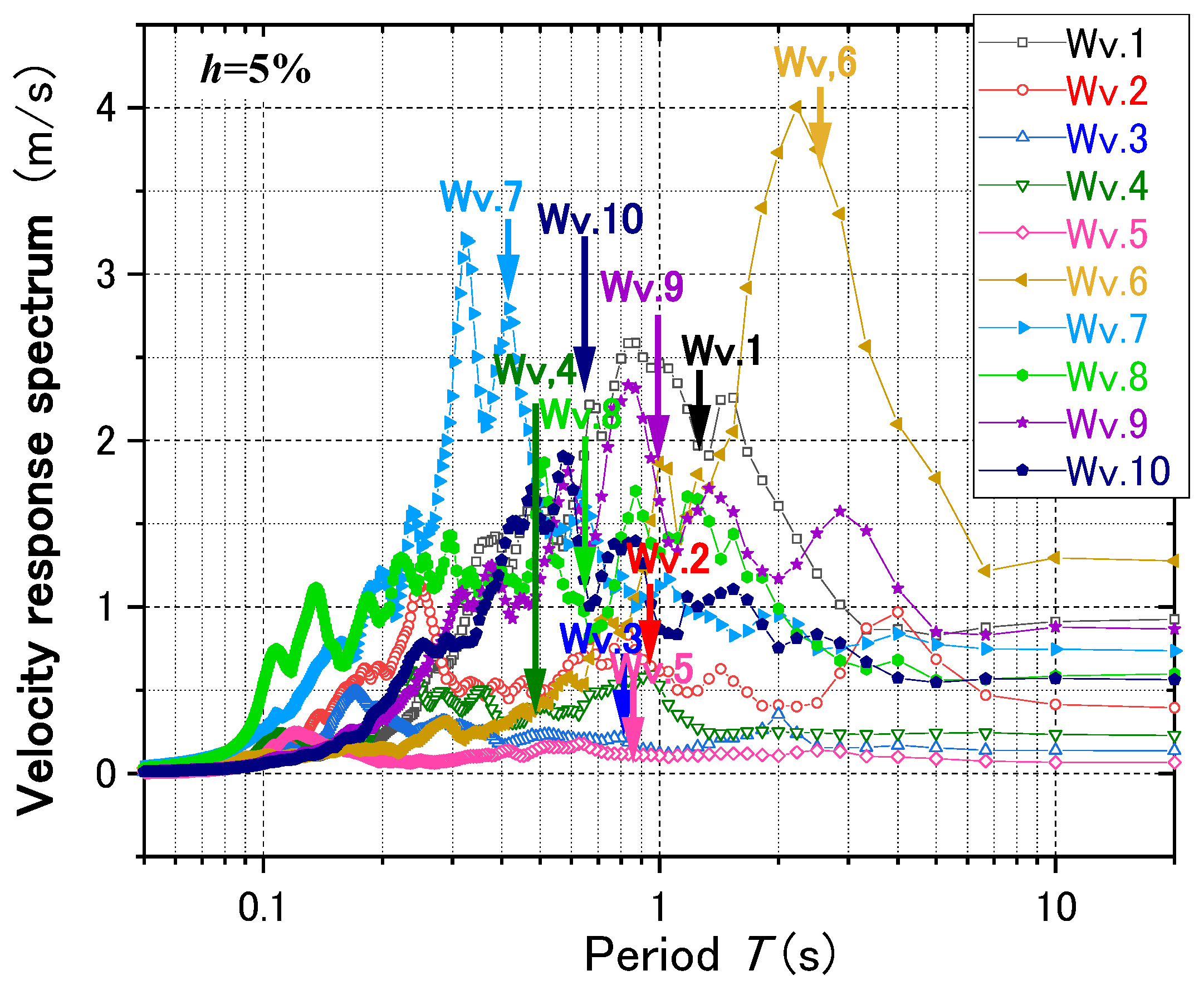
All acceleration records were processed using a band-pass filter (BPF) with the period band of 0.1–5 s. The portion of each record used in the analysis spans from the onset of the SH wave to the final point where residual acceleration falls within 4–8% of the peak. Figure 6 presents the velocity response spectra, which capture long-period motions critical to slope failure better than acceleration spectra. The spectral peak periods of the records range from 0.2 to 2.0 s and can be categorized into two groups: Group 1 (Wv.1, Wv.6~Wv.10) with isolated sharp peaks, and Group 2 (Wv.2~Wv.5) with broad, multi-spectral dull peaks. Slope parameters used in the analysis are consistent with those applied to harmonic wave cases: friction angle $\varphi$ = 35°, inclination angle difference $\varphi -\theta$ = 5°, sliding depth D = 5 m, initial displacement ratio D₀/D = 0.12, unit weight ρ = ρ_s = 1.8 t/m³, and shear wave velocity V_s = 200 m/s.

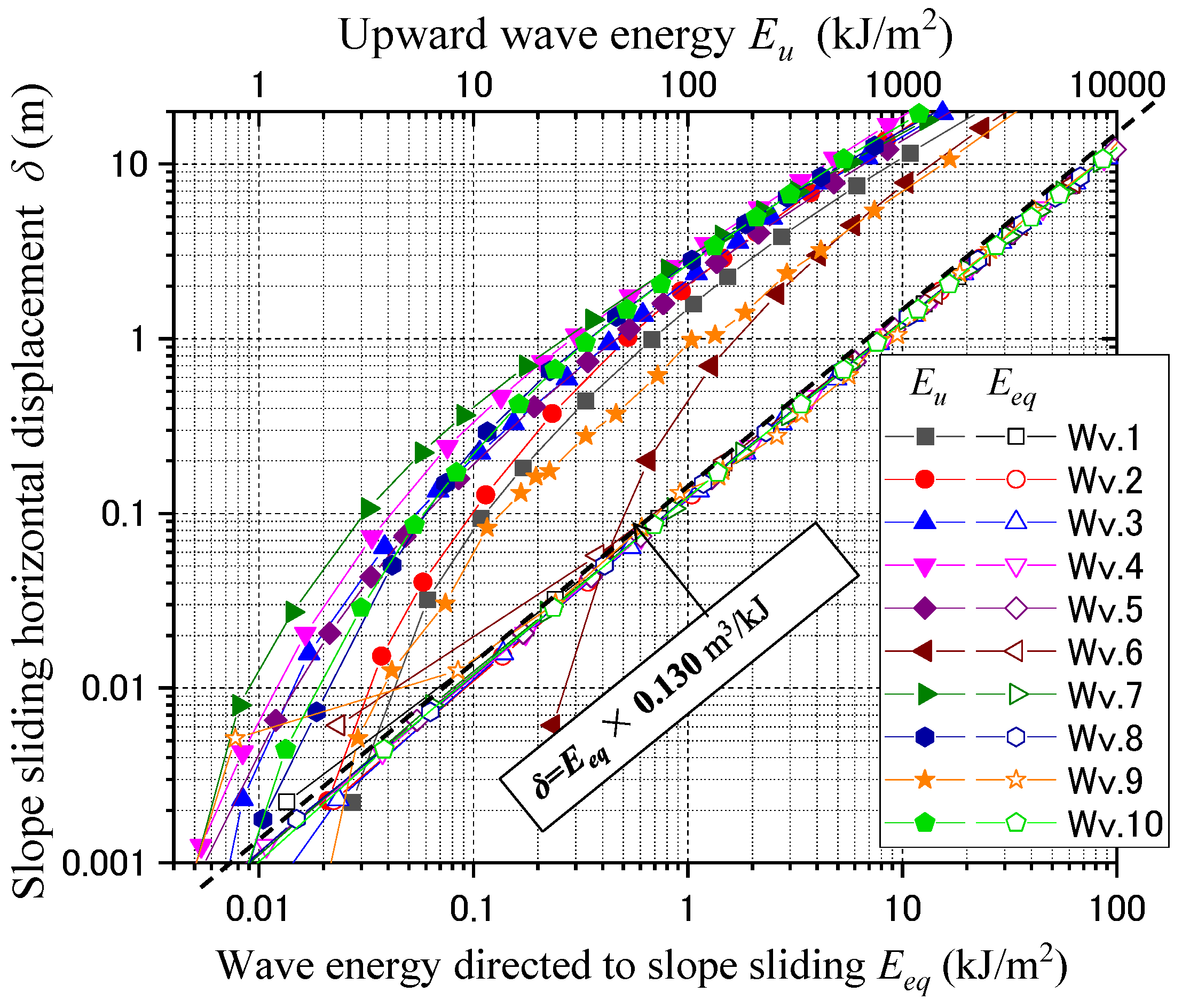
Figure 7 illustrates the relationship between sliding displacements δ and upward wave energies E_u or earthquake energies E_eq on a log-log scale. For individual earthquakes, input amplitudes were scaled stepwise, and results are plotted using line-connected symbols. While δ–E_u plots (solid symbols) vary significantly across the earthquakes, δ–E_eq plots (open symbols) are unified, aligning closely with the theoretical expression given in Equation (6). This highlights the unique role of E_eq in governing δ, independent of wide differences in amplitude, frequency content, irregularity, or duration. To leverage this uniqueness, however, E_eq or the ratio E_eq/E_u must be evaluated from E_u in advance.

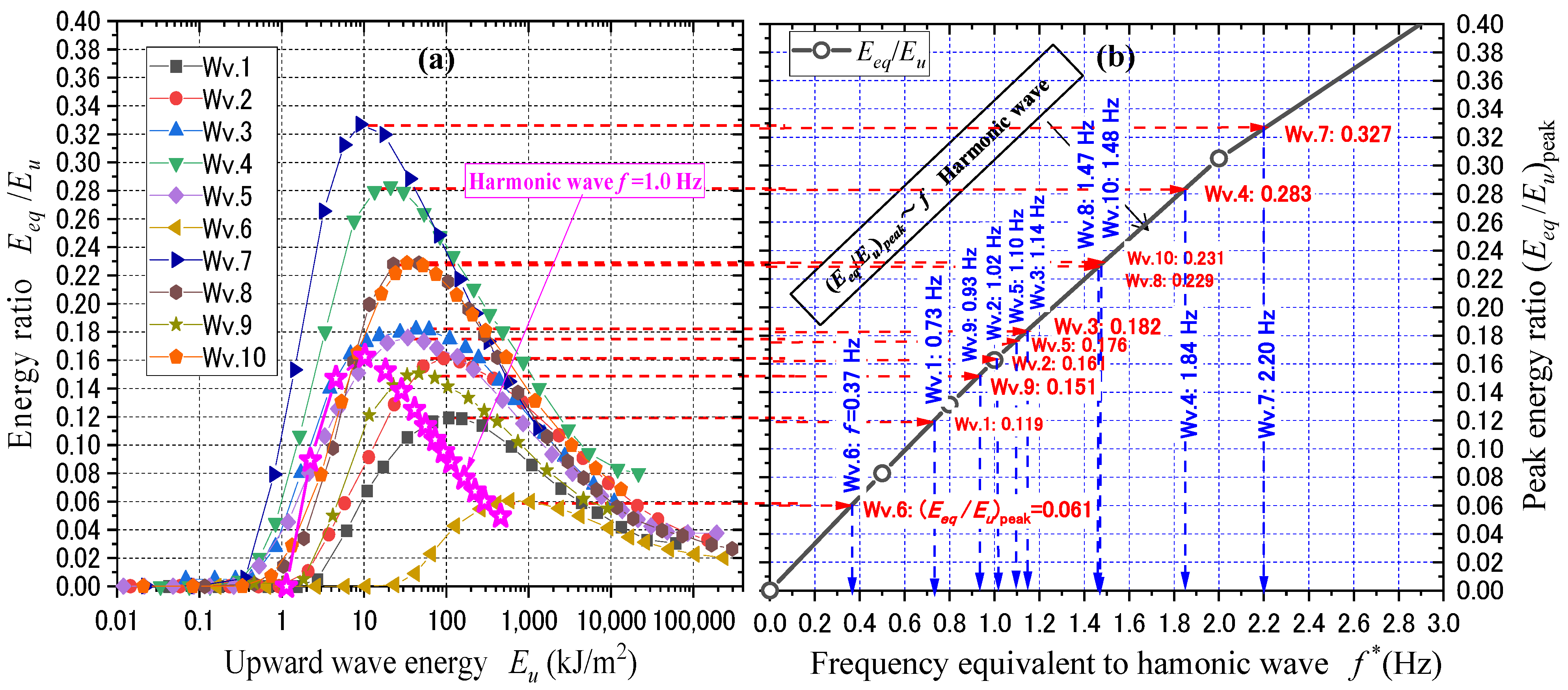
Figure 8a shows the semi-log plot of E_eq/E_u versus E_u for the ten records. Star symbols represent analogous results for harmonic motion at f = 1.0 Hz (see Figure 4). The E_eq/E_u~E_u curves for earthquake records resemble those of harmonic waves: rising from zero, peaking, and then declining. The peak values of E_eq/E_u range from 0.06 to 0.33, with higher peaks occurring at lower E_u-values, a trend also observed in Figure 4 for harmonic cases, where frequency plays a key role.

To explore this frequency dependency, the peak E_eq/E_u-values from Figure 8a are compared in Figure 8b with a reference curve, which is drawn by combining the peak values of E_eq/E_u for harmonic motions of different frequencies f in Figure 4. By projecting each peak value in Figure 8a horizontally to the reference curve in Figure 8b, equivalent frequencies f * are read off in Figure 8b corresponding to individual earthquake records. These f *-values and corresponding periods T* = 1/f * are listed in Table 1 and also indicated with arrows in the velocity spectra of Figure 6. The periods thus obtained are mostly consistent with the spectral peaks, though exact matches are difficult, suggesting that E_eq/E_u~E_u in irregular records mimics the frequency-dependent trend of harmonic waves.

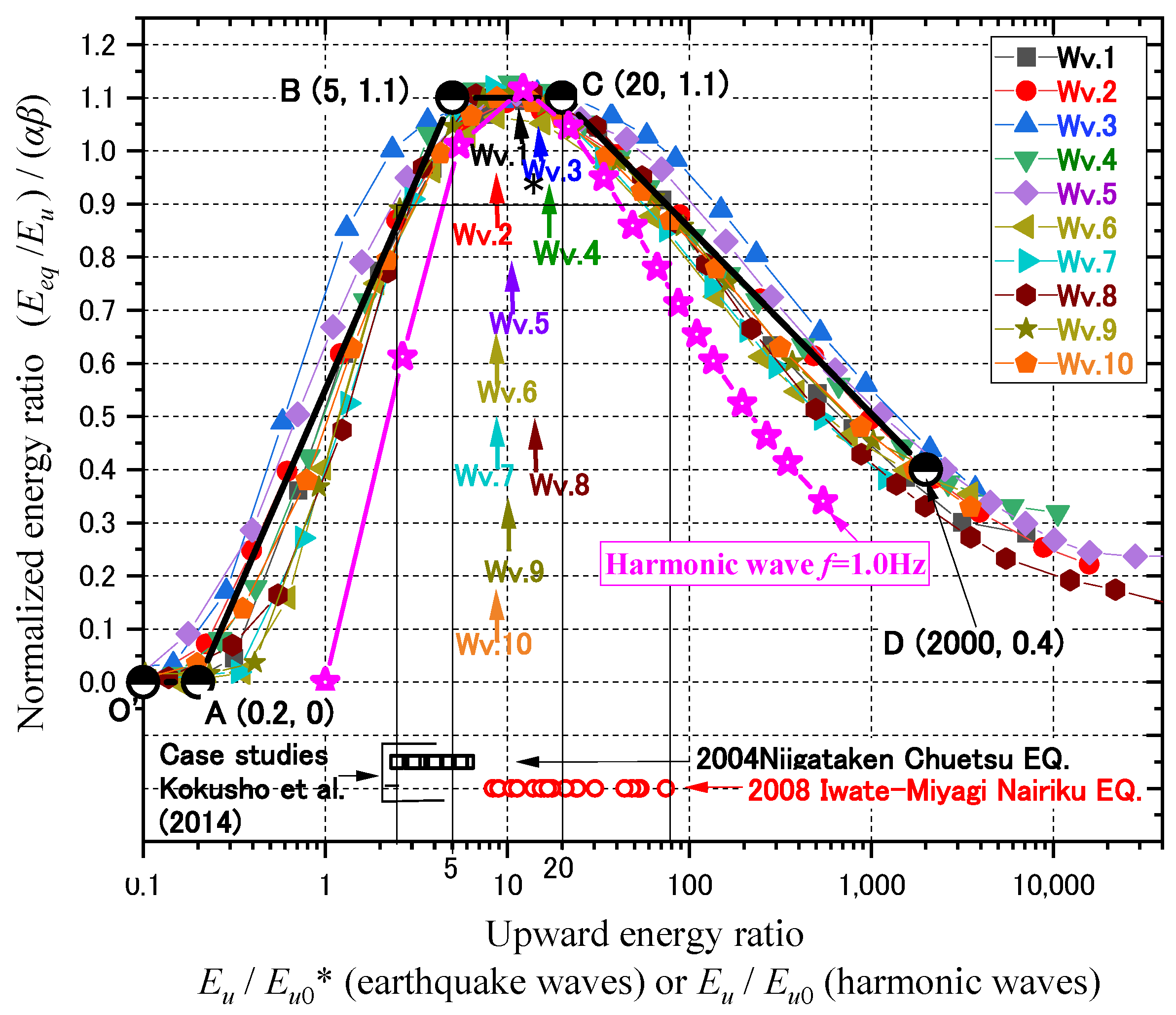
In Figure 5, the E_eq/E_u-ratio for harmonic waves was normalized using parameters α and β in Equations (19) and (20) to yield a frequency-insensitive metric: (E_eq/E_u)/(αβ). The same normalization applied to the E_eq/E_u-ratio calculated for the earthquake waves using their respective equivalent frequencies f * yields the vertical coordinates (E_eq/E_u)/(αβ) in Figure 9, where the peak values are nearly identical across the ten waves with mean ± SD = 1.10 ± 0.014, confirming the effectiveness of this normalization.

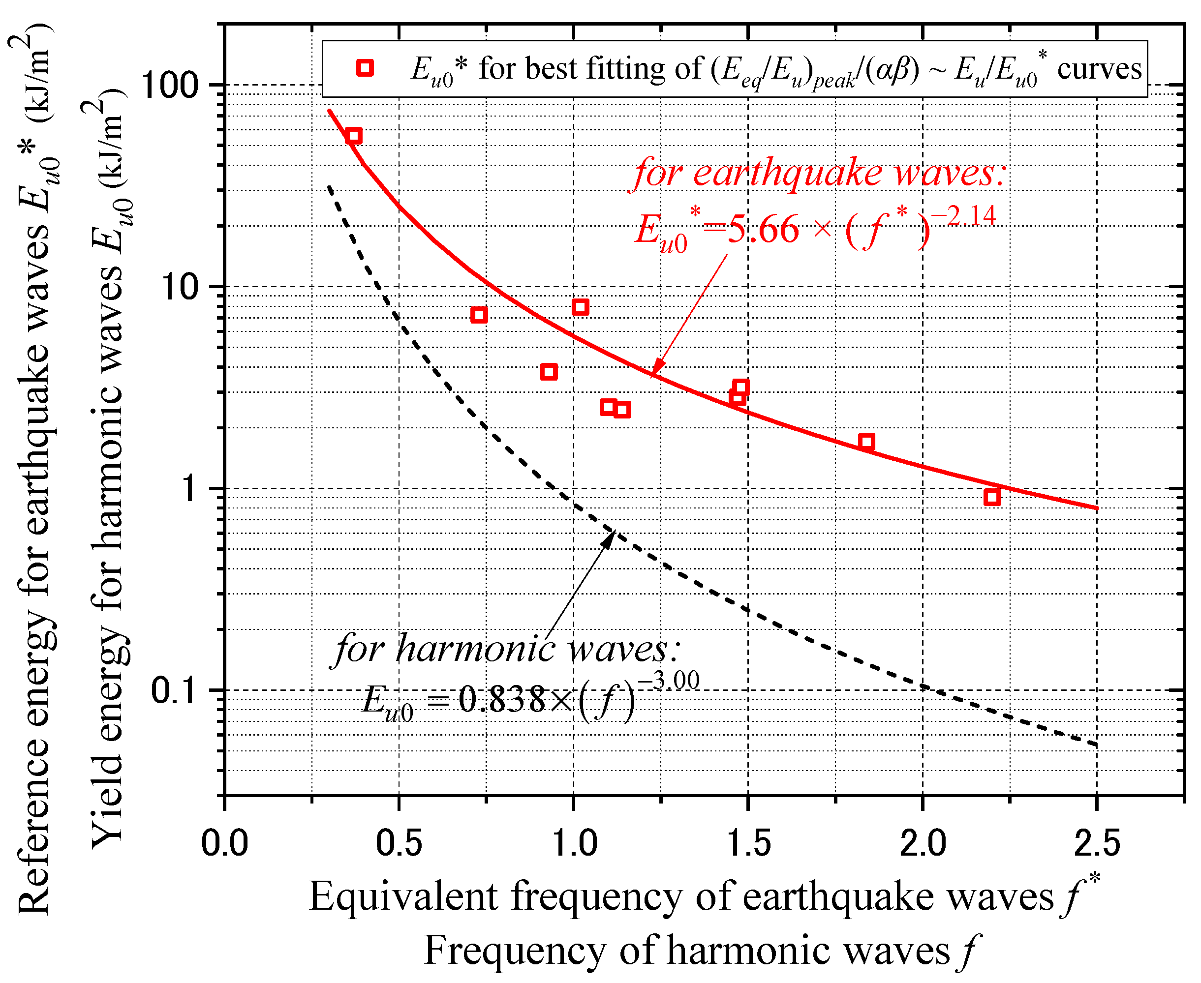
To normalize the horizontal axis, too, reference energies E_u0* are introduced such that (E_eq/E_u)/(αβ)~E_u/E_u0* curves are unified as closely as possible with the harmonic wave of f = 1.0 Hz shown with the star symbols. The E_u0* values thus optimized are plotted against the equivalent frequencies f * in Figure 10 (open squares), forming a regression curve with R² = 0.90.

$${E_{u0}}^{*}=5.66\times {\left(f^{*}\right)}^{-2.14}$$

(21)

For comparison, E_u0-values, yield energies for harmonic waves corresponding to yield acceleration gtan($\varphi -\theta$), calculated from Equation (12) are also plotted (the dashed line) [12].

$$E_{u0}={\rho }_s{V}_s{g}^2/\left(32{\pi }^2{f}^3\right)\times {\tan }^2\left(\varphi -\theta \right)=0.838\times {\left(f\right)}^{-3.00}$$

(22)

Although E_u0* lacks a logical definition due to the randomness of earthquake motions, its similarity to E_u0 in the monotonic decrease with increasing frequency as a power function suggests a similar role in triggering slope failure.

The normalized plots in Figure 9 reveal a unified pattern across all earthquake waves: a plateau near E_u/E_u0* ≈ 10, flanked by ascending and descending slopes. Compared to harmonic waves, earthquake records exhibit gentler slopes and broader plateaus, especially for Wv.3 and Wv.5, which have flat spectra (Figure 6). This is likely due to E_u0* reflecting a spectrum of multiple peaks rather than a single peak. In harmonic cases, sliding initiates at E_u/E_u0 = 1.0 [12], consistent with the yield energy definition in Equation (22). For earthquake records, sliding tends to begin at E_u/E_u0* ≈ 0.1~0.4, reflecting the lack of a clear yield threshold. Despite these differences, the normalized chart in Figure 9 successfully integrates the diverse E_eq/E_u~E_u/E_u0* relationships in Figure 8a.

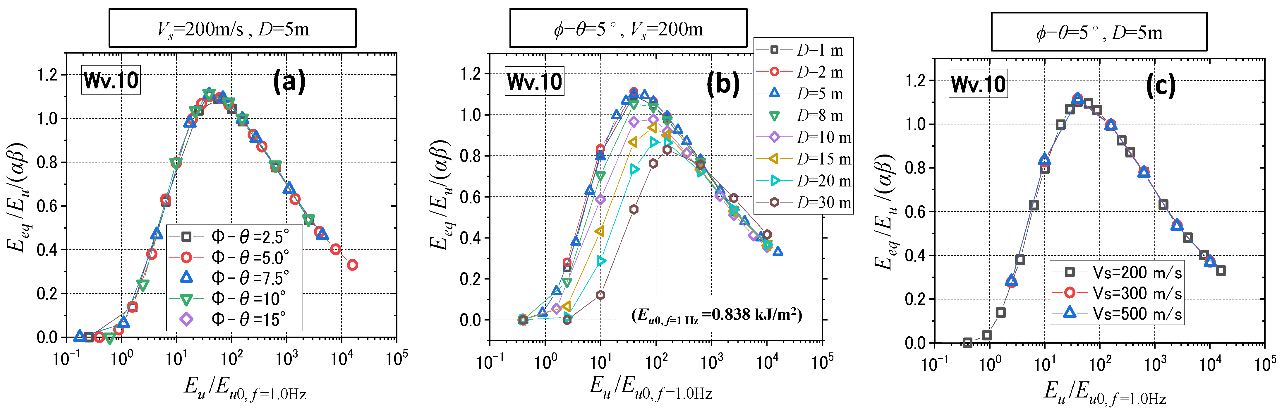
To assess parameter sensitivity, additional analyses are performed using Wv.10, by varying $\varphi -\theta$, D, and V_s. In Figure 11a, varying $\varphi -\theta$ from 2.5° to 15° yields consistent normalized curves, as both vertical and horizontal axes adjust accordingly. In Figure 11b, increasing D beyond 8 m introduces deviations: ~10% error in E_eq for D = 10 m and ~20% for D = 20 m. However, this is not critical, as E_eq is typically much smaller than gravitational energy E_gr in slides of large D [10,11], leading to the evaluation error in E_eq being less significant in the energy balance in Equation (2). In Figure 11c, variations in V_s have a negligible impact on the normalized correlation.

5. Unified Slope Slide Evaluation for Arbitrary Motions

The correlation between (E_eq/E_u)/(αβ) and E_u/E_u0*, as shown in Figure 9, provides a convenient framework for evaluating E_eq directly from E_u. These nearly unified curves for ten earthquake records can be approximated by a set of broken lines (OABCD) on a semi-logarithmic graph and formulated in Equation (23):

$$\left.\begin{array}{ccc}\mathrm{OA}:& E_u/E_{u0}^{*}\le 0.2& E_{eq}/E_u/\left(\alpha \beta \right)=0\\ \mathrm{AB}:& {0.2<E_u/E_{u0}}^{*}\le 5.0& E_{eq}/E_u/\left(\alpha \beta \right)=1.58\cdot {\log }_{10}\left(E_u/E_{u0}^{*}\right)\\ \mathrm{BC}:& 5.0<E_u/E_{u0}^{*}\le 20& E_{eq}/E_u/\left(\alpha \beta \right)=1.10\\ \mathrm{CD}:& 20<E_u/E_{u0}^{*}\le 2000& E_{eq}/E_u/\left(\alpha \beta \right)=-0.35\cdot {\log }_{10}\left(E_u/E_{u0}^{*}\right)+1.56\end{array}\right\}$$

(23)

Using this formulation, steps to evaluate slope sliding energy E_eq and displacement δ for arbitrary design earthquakes are as follows:

(1)

If design acceleration waves ${\ddot{u}}_0\left(t\right)$ in Equation (10) are available for direct input motions to slopes, the upward SH-waves may be approximated as ${\ddot{u}}_1\left(t\right)={\ddot{u}}_0\left(t\right)/2$ by assuming complete reflection at the soil surface. The upward energy E_u can then be calculated from Equation (12) using upward velocity waves, ${\dot{u}}_1\left(t\right)={\displaystyle \int {\ddot{u}}_1\left(t\right)}dt$, and the predominant frequency f_p is determined from the response spectrum of ${\dot{u}}_1\left(t\right)$.

(2)

If design motions are unavailable, begin by selecting the earthquake magnitude M and hypocenter distance R (in meters). The input wave energy E_ip (in kJ/m²) at a bedrock can be roughly estimated using the wave energy radiation principle [15] and the empirical formula by Gutenberg [16]:

$$E_{ip}=E_0/\left(4\pi R^2\right)$$

(24)

$$\log E_0=1.5M+1.8$$

(25)

For greater accuracy, fault and path mechanisms of particular earthquakes should be considered to modify the energy if possible. The predominant frequency f_p, inversely correlated with M (e.g., Aki [17]), may be predicted according to regional earthquake databases. The upward energy E_u for a specific slope is then determined from E_ip using the S-wave impedance ratio between the layer beneath the slope and the bedrock $\left({\rho }_s{V}_s\right)/\left({\rho }_{sb}{V}_{sb}\right)$ as

$$E_u=E_{ip}\times {\left[\left({\rho }_s{V}_s\right)/\left({\rho }_{sb}{V}_{sb}\right)\right]}^{0.7}/2$$

(26)

This empirical relation, developed by Kokusho & Suzuki [15], is based on numerous strong motion records from vertical arrays in Japan. The division by 2 in the equation accounts for the average contribution of horizontal SH-wave energy in the sliding direction [11].

(3)

The reference energy E_u0* is calculated by substituting the predominant frequency f_p into the equivalent frequency f * in Equation (21). Slope parameters $\theta$, $\varphi$, V_s, ρ, and D are then used to compute α and β in Equations (19) and (20). With the horizontal coordinate E_u/E_u0*, the vertical coordinate (E_eq/E_u)/(αβ) is read off from Figure 9 or calculated using Equation (23). For E_u/E_u0* < 0.2, where E_eq/E_u = 0, slopes may be considered stable, though minor variability may be possible. Otherwise, a positive E_eq leads to a non-zero displacement δ, which is readily obtained from Equation (6).

In Figure 9, the vertical coordinate (E_eq/E_u)/(αβ) ranges from 0 to 1.10 as the horizontal coordinate E_u/E_u0* spans from approximately 0.2 to over 1000. This indicates that the energy E_eq directed toward slope sliding varies significantly with upward energy. The ten earthquake records in Table 1 used here are all strong motions obtained in damaged areas, some including actual slope failures. Arrows in Figure 9 mark the normalized upward energies E_u/E_u0* all falling between 5 and 20 for Wv.1 to Wv.10 within the plateau section BC, suggesting that typical strong motions in Japan tended so far to yield (E_eq/E_u)/(αβ) = 1.10.

Among the ten events, the 2004 Niigataken Chuetsu and 2008 Iwate-Miyagi Nairiku earthquakes triggered numerous slope failures in mountainous terrains. Case studies on affected slopes during the events exhibited runout distances ranging from a few to over 100 m [10,11,18]. The corresponding E_u/E_u0* values for these slopes (plotted with two-type open dots at the bottom of Figure 9) range from 2.5 to 80, yielding the values (E_eq/E_u)/(αβ) between 0.90 and 1.10. Hence, this range seems to be representative in field observations and aerial imagery during the two events. According to Figure 9, slope sliding initiates at E_u/E_u0* = 0.2, where E_eq and δ start to be positive. The gap between 0.2 and 2.5 may be considered as a transition zone where minor cracking evolves into meaningful displacements.

Consequently, the EBNM offers a significant benefit for risk analysis of earthquake-induced slope failures in hilly and mountainous regions. Though slopes are sometimes approximated by circular slope models in practice, the infinitely long straight slope condition assumed here may fit natural slopes better because of intrinsic geological structures and be suited to zonation studies on co-seismic slope sliding covering wider regions. Unlike the CNM, it does not require time-domain acceleration inputs for each slope. Instead, it accommodates diverse slope gradients, shear strengths, and earthquake scenarios simply through parametric variations. Hence, it is well-suited for probabilistic risk assessments, seismic zonation studies, and screening tasks for system vulnerabilities of infrastructures such as roads, railways, and utility pipelines traversing mountainous terrains.

6. Summary

The Energy-Based Newmark Method (EBNM) has been applied to ten widely varied earthquake motions to evaluate slope displacements of infinitely long slopes with variable parameters. This study has led to the development of a unified methodology for determining slope sliding displacements for arbitrary earthquake inputs without conventional numerical calculations, yielding the following key findings:

(i)

Slope displacement δ is uniquely expressed by the earthquake energy directed toward slope sliding E_eq using a simple formula: $\delta =E_{eq}/\left[\rho gD\tan \left(\varphi -\theta \right)\right]$ where $\varphi$ = the friction angle, $\theta$ = the slope angle, ρg = the unit weight, and D is the thickness of the sliding block. This relationship holds irrespective of acceleration, duration, or frequency content of earthquake motions. The energy E_eq is defined as the difference between upward and downward wave energies beneath the slope: E_eq = E_u−E_d.

(ii)

Energy ratio E_eq/E_u tends to rise with increasing upward energy E_u from zero at the onset of sliding, reach a peak, and then decline monotonically. Despite the differences in the E_eq/E_u∼E_u correlations across different earthquake waves, which are found to be mainly attributable to differences in predominant frequency f_p, they basically share the same trend.

(iii)

The correlations have been reformulated as (E_eq/E_u)/(αβ)∼E_u/E_u0*, where α and β are slope/frequency-dependent constants, and E_u0* is a reference energy depending on predominant frequency f_p. This unified relationship is represented by a set of broken lines (OABCD) on a design chart or by Equation (23). Once E_u is known, E_eq/E_u can be obtained from the chart, and δ can be readily calculated from E_eq using the key formula, Equation (6).

(iv)

The upward energy E_u can be calculated from design acceleration motions in Equation (12), if available. Otherwise, it may be estimated using empirical formulas based on earthquake magnitude M and hypocenter distance R, assuming spherical energy radiation. In case histories of earthquakes, the normalized energy values E_u/E_u0* for damaged slopes ranged from 2.5 to 80, corresponding to (E_eq/E_u)/(αβ) = 0.9–1.1. The chart also indicates that slope sliding initiates at E_u/E_u0* ≈ 0.2. The gap between 0.2 and 2.5 may represent an energy allowance where minor fissures evolve into measurable displacements.

In conclusion, the EBNM offers significant benefits for risk analysis of earthquake-induced slope failures in hilly and mountainous terrains. Unlike the Conventional Newmark Method (CNM), it does not require time-domain numerical analyses using acceleration inputs for individual slopes. Instead, it accommodates diverse slope conditions and earthquake scenarios by adjusting the relevant parameters. The method is well-suited for probabilistic risk assessments, seismic zonation studies by local authorities, and contingency planning for infrastructure such as roads, railways, and pipelines in mountainous regions.

Nevertheless, despite its potential for simplified seismic slope stability evaluations, validation studies remain limited, though this applies to the CNM as well. To enhance the credibility of the EBNM, it is essential to accumulate and analyze case history data, comparing the observed failures with the predictions. Such efforts will help clarify the method’s strengths and limitations and promote its acceptance in the engineering community.