Interpretable AI-Driven Modelling of Soil–Structure Interface Shear Strength Using Genetic Programming with SHAP and Fourier Feature Augmentation

Abstract

Accurate prediction of soil–structure interface shear strength (τ_max) is critical for reliable geotechnical design. This study combines experimental testing with interpretable machine learning to overcome the limitations of traditional empirical models and black-box approaches. Ninety large-displacement ring shear tests were performed on five sands and three interface materials (steel, PVC, and stone) under normal stresses of 25–100 kPa. The results showed that particle morphology, quantified by the regularity index (RI), and surface roughness (R_t) are dominant factors. Irregular grains and rougher interfaces mobilised higher τ_max through enhanced interlocking, while smoother particles reduced this benefit. Harder surfaces resisted asperity crushing and maintained higher shear strength, whereas softer materials such as PVC showed localised deformation and lower resistance. These experimental findings formed the basis for a hybrid symbolic regression framework integrating Genetic Programming (GP) with Shapley Additive Explanations (SHAP), Fourier feature augmentation, and physics-informed constraints. Compared with multiple linear regression and other hybrid GP variants, the Physics-Informed Neural Fourier GP (PIN-FGP) model achieved the best performance (R² = 0.9866, RMSE = 2.0 kPa). The outcome is a set of five interpretable and physics-consistent formulas linking measurable soil and interface properties to τ_max. The study provides both new experimental insights and transparent predictive tools, supporting safer and more defensible geotechnical design and analysis.

1. Introduction

Shear strength at the soil–structure interface is a critical design parameter in geotechnical engineering [1]. It dictates load transfer mechanisms in shallow and deep foundations, retaining walls, piles, soil nails, geosynthetics, and other structures embedded in or interacting with the soil [2,3,4]. Hence, predicting an accurate magnitude is crucial for the ensuring stability, serviceability and durability of an engineered system. For interface behaviour, there is a level of complexity given by the interactions between particle morphology/grading/density, the surface roughness and the material hardness used in both the soil and the structure, as well as the amount of normal stress applied, which in turn impact the peak and residual shear resistance [5,6,7].

Experimental investigations utilising direct shear and ring shear devices have traditionally contributed important knowledge regarding these mechanisms. Uesugi and Kishida [2] were amongst the first to systematically quantify the effect of interface roughness on the friction between sand and steel. Their factorial experiments helped to show that roughness and sand type were significant in defining shear resistance, and that the other parameters (e.g., D₅₀, normal stress) were also important but more context-dependent. The follow-up micro-mechanical study conducted by Dove and Frost [3] classified dilative rough interfaces and non-dilative smooth interfaces, thus demonstrating the mechanical interlocking and deformation of rough interfaces.

The modified torsional ring shear apparatus has become a preferred testing device for large-displacement interface behaviour, eliminating the displacement constraints and edge effects of direct shear tests [8,9,10,11,12,13]. Bromhead [4] adapted the ring shear test to ameliorate the representation of residual strengths and capture laboratory test results representative of field experiences in slow-moving landslides and long-term soil–structure interactions. This device allows researchers to reliably capture both peak and residual shear strength without the boundary effects experienced in other devices.

The shear behaviour of interfaces is very sensitive to the differences in the materials. Research has shown that harder interfaces (e.g., stone, high-hardness steel) tend to limit the crushing of asperities to develop high effective friction angles, while soft materials (e.g., PVC) tend to show localised plastic deformation that will lead to reduced shear resistance under the same normal load [14,15,16,17]. Rate dependency and cyclic degradation also complicate this picture, with studies showing that low normal stress at smooth interfaces is still rate dependent, while rough, dilative interfaces show decreasing rate dependency under higher normal stress [18,19,20,21].

In recent years, research on geosynthetic–soil interfaces, particularly between geogrids and sandy soils, has expanded our understanding of frictional behaviour and interlocking mechanisms. Geogrid–soil interaction is governed not only by surface friction but also by passive resistance and soil interlocking within geogrid apertures, particularly across transverse ribs [22,23]. Large-scale direct shear tests have shown that while soil–rib friction is dominant, transverse ribs can contribute an additional portion of the ultimate interface shear strength depending on rib stiffness and aperture size [21]. These results highlight the combined role of friction, aperture geometry, and passive bearing mechanisms in geogrid–soil interfaces.

The influence of geogrid reinforcement on foundation systems, such as strip footings on reinforced sand, further demonstrates the engineering significance of these interface mechanisms. Both experimental and numerical studies confirm that geogrids enhance bearing capacity and load distribution, particularly when reinforcement depth and configuration are optimised [23,24]. For example, studies on strip footings placed over geogrid-reinforced sand have shown marked improvements in bearing capacity and settlement performance, underscoring the importance of explicitly modelling interfacial interlocking and friction in order to advance practical geotechnical design.

The geometry and dimensions of shear testing devices strongly influence the measured interface response. Direct shear boxes are typically small (60–100 mm), which may exaggerate boundary effects and constrain displacement, limiting their ability to capture residual strength and progressive failure. In contrast, ring shear devices allow for continuous displacement and minimise edge effects, providing more representative residual strengths. Nevertheless, even the annular geometry of ring shear tests is much smaller than real soil–structure interfaces, which often extend over meters or tens of meters. These dimensional effects can influence mobilised shear strength, dilatancy, and residual behaviour, and must be considered when interpreting laboratory results for field applications [4,11].

While the Mohr–Coulomb approach for classical empirical models has been commonly used to derive estimations for interface shear strength, the linear assumptions of these models cannot capture the nonlinear, multivariate interactions as described earlier [25,26]. This inconsistency has led the geotechnical community to develop and apply artificial intelligence (AI) and machine learning (ML) models, which can represent complex, nonlinear relationships, to solve these problems. In the past 10 years, AI has been deployed for prediction of parameters like shear strength, friction angle, swelling pressure, and settlement [27,28,29,30,31].

Table 1. Literature Review Comparison.

Reference	Study Type & Method	Dataset/Specimen	Target/Output	Gap vs. This Paper	Advantages of This Paper
Uesugi and Kishida [2]	Experimental; direct shear on sand–mild steel	Dry sands; steel interfaces with varied	Frictional resistance at yield/interface	No interpretable AI; limited multivariate, data-driven	Builds a multi-material ring shear dataset
Dove and Frost [3]	Experimental; particle-scale/geomembrane–particle interface tests	Smooth geomembrane–particle interfaces	Peak friction behaviour and dilative/non-dilative	Mechanistic insight but no predictive, interpretable	Transforms multi-feature measurements (RI, D50, Cu, etc.)
Bromhead [4]	Method development; ring shear apparatus	Device concept for large-displacement shear	Ability to measure peak and residual	No modelling framework; apparatus-level contribution only	Uses a modified ring shear
Stark and Vettel [10]	Testing procedure; Bromhead ring shear test	Standardised protocol	Procedural guidance for residual shear measurements	No data-driven model or interpretability approach	Extends beyond procedure to deliver validate
Liu et al. [5]	Data resource; unified database of ring	Sandy–silty soils; steel interfaces	Compiled ring shear data	Database focus; not an interpretable AI	Collects new multi-material data (steel, PVC
Farhadi & Lashkari [8]	Experimental; interface shear with inherent anisotropy	Crushed sand–steel interfaces; anisotropy effects	Shear behaviour, anisotropy influence	Focus on anisotropy; does not produce	Covers broader variable set and yields
Dove et al. [9]	Experimental; particle-scale surface interactions for non-dilative	Non-dilative interface systems	Micro-mechanics of surface interaction	Mechanistic focus without global predictive model	Bridges mechanics and data via interpretable
Eid [24]	Experimental; geosynthetic composite system shear	Geosynthetic composites	Shear strength for design	Material/system-specific; no interpretable AI	General framework applicable to diverse interfaces
Tanga [32]	Machine learning; Random Forest with SHAP	495 geomembrane–soil interface tests	Interface friction angle/τmax proxies	Strong accuracy but black-box; lacks explicit	Provides symbolic formulas (GP hybrids), SHAP-guided
This paper (PIN-FGP, FF-GP, SHAP-GP, NGBoost-GP)	Hybrid symbolic regression with physics-informed constraints	90 large-displacement ring shear tests; 5 sands	Predict τmax with interpretable, compact equations	nan	State-of-the-art accuracy with transparent equations; uncertainty

shows a literature review comparison.

In relation to soil–structure interfaces specifically, Random Forest (RF) and gradient boosting models have demonstrated good predictive power. Tanga [32] identified 495 geomembrane–soil interface tests and found good predictions of the interface friction angle using RF, and SHAP (Shapley Additive Explanations) analysis identified surface type, normal stress, and soil state as meaningful features. For the sand–continuum datasets, a similar analysis showed that RF performed better than multiple linear regression (MLR) in predicting maximum shear stress [32,33].

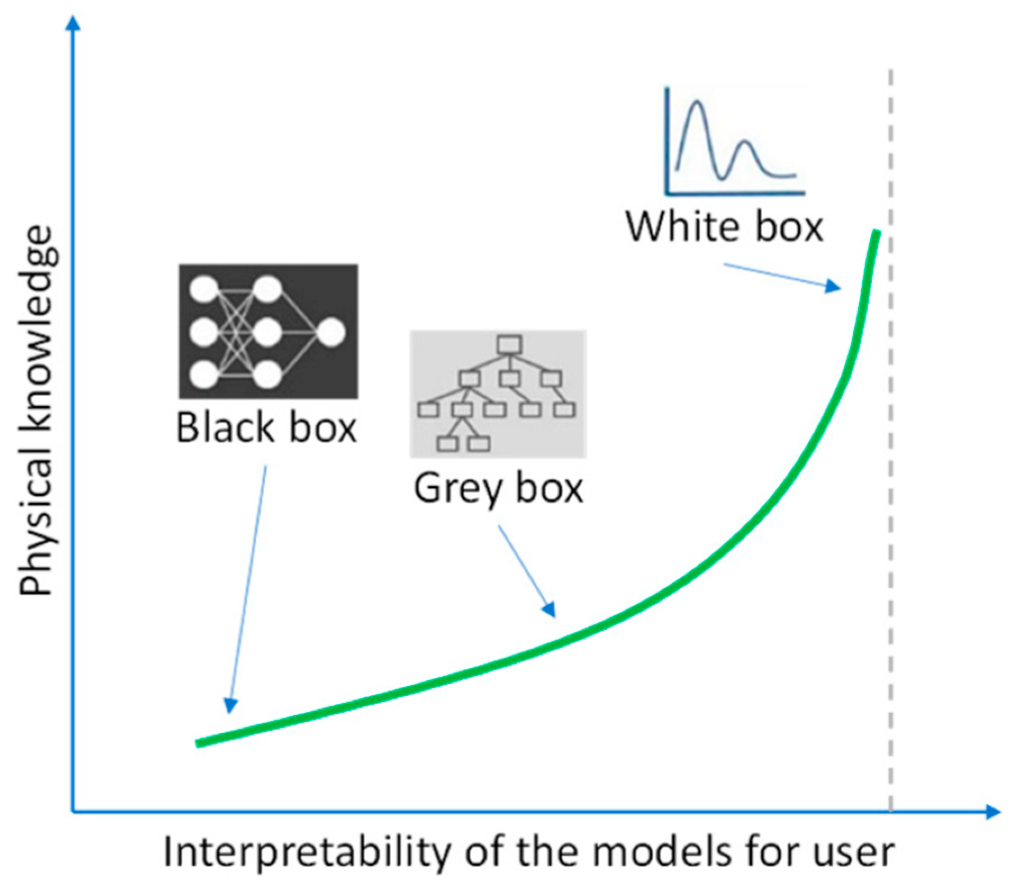
AI algorithms have faced scepticism in geotechnical modelling due to the limited transparency of many data-driven approaches [34]. As illustrated in Figure 1, models can be classified as black-box, grey-box, or white-box depending on their interpretability and incorporation of physical knowledge [35]. In this study’s context, black-box methods (e.g., ANN) provide strong predictive accuracy but lack interpretable structure, whereas white-box models are derived from first principles. The proposed hybrid GP-based methods operate in the grey-box domain, evolving explicit mathematical expressions that balance accuracy with interpretability, enabling the extraction of meaningful physical insights from complex soil–structure interface shear data while outperforming purely black-box approaches.

Although these black-box models may provide excellent accuracy, they do not always provide an interpretation, a necessary element for engineering acceptance. Subsequently, there has been increasing interest in symbolic regression (SR) with Genetic Programming (GP), a process that can automatically evolve explicit mathematical expressions from data [38,39,40]. SR has the ability to produce an interpretable formula that can be readily implemented in design; good predictive accuracy is also maintained [41,42,43,44].

In the last few years, scientists have looked at hybrid GP approaches that combine other AI techniques to improve robustness and interpretability. Although there has not been a large body of work on hybrid GP approaches, NGBoost and GP are relatively well-known hybrids that incorporate probabilistic ensemble learning and provide users with the ability to quantify uncertainty while also obtaining symbolic formulae [45]. SHAP and GP are another variant of hybrids that use feature importance rankings to help guide the symbolic search process. This reduces noise for search stability [46,47]. Fourier Feature-Augmented GP (FF-GP) combines trigonometric transformations with GP and can model oscillatory or periodic effects that could arise from asperity-scale interactions or cyclical loading [48].

Physics-Informed Neural Networks (PINNs) and physics-regularised GP variants push this further by integrating domain knowledge, ensuring learned relationships are compliant with basic mechanical constraints (e.g., normal stress should increase shear strength monotonously) [49,50]. These can stop some unphysical predictions but in a manner that is still reasonable. Research in adjacent geotechnical topics, e.g., tunnelling-induced settlement and soil deformation modelling, has shown that physics-informed constraints enhance generalisation [51,52,53,54].

Although machine learning methods such as Random Forest, artificial neural networks, and gradient boosting have demonstrated strong predictive capability for soil and interface behaviour, they are predominantly black-box models. Their lack of interpretability and physics-awareness limits engineering acceptance, while traditional approaches such as Mohr–Coulomb or linear regression are too simplistic to capture the nonlinear, multivariate interactions at soil–structure interfaces. This highlights a clear gap for models that combine predictive power with transparency and physical consistency.

To address this, the present study develops a comprehensive hybrid symbolic regression framework based on Genetic Programming (GP). The framework integrates SHAP-guided feature selection, Fourier feature augmentation, and physics-informed constraints, and is evaluated alongside multiple linear regression (MLR), NGBoost–GP, SHAP–GP, PIN-FGP, and FF-GP models. A systematically curated database of 90 large-displacement ring shear tests on five sands and three interface materials under different normal stresses provides the foundation for rigorous model training and validation.

The outcome of this work is a set of compact, interpretable, and physics-consistent predictive formulas that advance beyond black-box AI approaches. By directly linking measurable physical characteristics such as roughness, hardness, morphology, and grading to interface shear strength, these models enable more transparent and defensible geotechnical decision-making. Their applications span foundation design, forensic assessments, and performance-based engineering, bridging the gap between academic innovation and practical geotechnical practice.

2. Materials and Methods

This section details the experimental setup, data acquisition methods, computational modelling methods used to investigate and to predict soil’s shear strength based on the ring shear test data. The methods are separated into subsections for the material selection, the experimental equipment and evaluation methods, data processing and description, and the symbolic and machine learning modelling methods.

2.1. Experimental Setup and Material Characterisation

Five different sand types (refer to Figure 2), each with different particle size distributions, shapes, and mineralogical characteristics, were chosen for testing. To quantify the particle morphology of the sands, roundness and sphericity measurements were captured, which were then normalised into a regularity index (RI), which is described as the ratio of roundness to sphericity. The RI is a key morphological parameter that could have effects on mechanical interlocking at the soil–continuum interface. This choice is consistent with recent reviews highlighting that particle shape fundamentally governs contact mechanics, stress distribution, and breakage susceptibility in granular materials, thereby influencing interface shear strength [50].

Particle roundness and sphericity were determined from high-resolution microscope images using ImageJ (version 1.54). Roundness was quantified by comparing grain edge curvature to a perfect circle, while sphericity was calculated from projected area and perimeter. The regularity index (RI) was then defined as the ratio of roundness to sphericity [3].

According to

Table 2. Properties of the granular materials used in the study.

Soil	Type	Gs	D50 (mm)	Cu	Cc	RI
A	Quartz Medium Sand	2.65	0.51	0.97	0.72	0.72
B	Quartz Coarse Sand	2.65	1.77	1.45	0.96	0.40
C	Quartz Well-Graded Sand	2.65	0.63	6.20	1.31	0.37
D	Granite Sand	3.75	0.51	1.20	0.97	0.64
E	Quartz Fine Gravel	2.65	1.72	1.69	1.01	0.41

, median particle size (D₅₀) and particle grading properties (e.g., coefficient of uniformity: C_u and coefficient of curvature: C_c), and porosity (n) were assessed to quantify general characteristics of granular assembly. Porosity was assessed based on dry density measurements from reproducible sample preparation procedures that produced loose and dense versions of the sands through controlled methodologies (e.g., sand raining) while adjusting the dropping height of sand into the testing mould. The loose versions were created through direct pouring (zero drop height), while the dense versions were created by ensuring sedimentation and densification (approximately 1 m drop height). This characterisation would ensure that the morpho-granular properties that govern shear behaviour were systematically incorporated.

The regularity index (RI) was quantified through image analysis of sand particles. Roundness and sphericity were measured from high-resolution microscope images using ImageJ (version 1.54), and RI was calculated as the ratio of roundness to sphericity, following the methodology of Dove and Frost [3]. In

Table 3. Sample initial density of all sands at loose and dense states.

Sand Type	A	B	C	D	E
Loose state (g/cm3)	1.65	1.64	1.74	2.22	1.66
Dense state (g/cm3)	1.72	1.83	2.03	2.42	1.73

, the loose state corresponds to the minimum dry density and the dense state corresponds to the maximum dry density for each sand type.

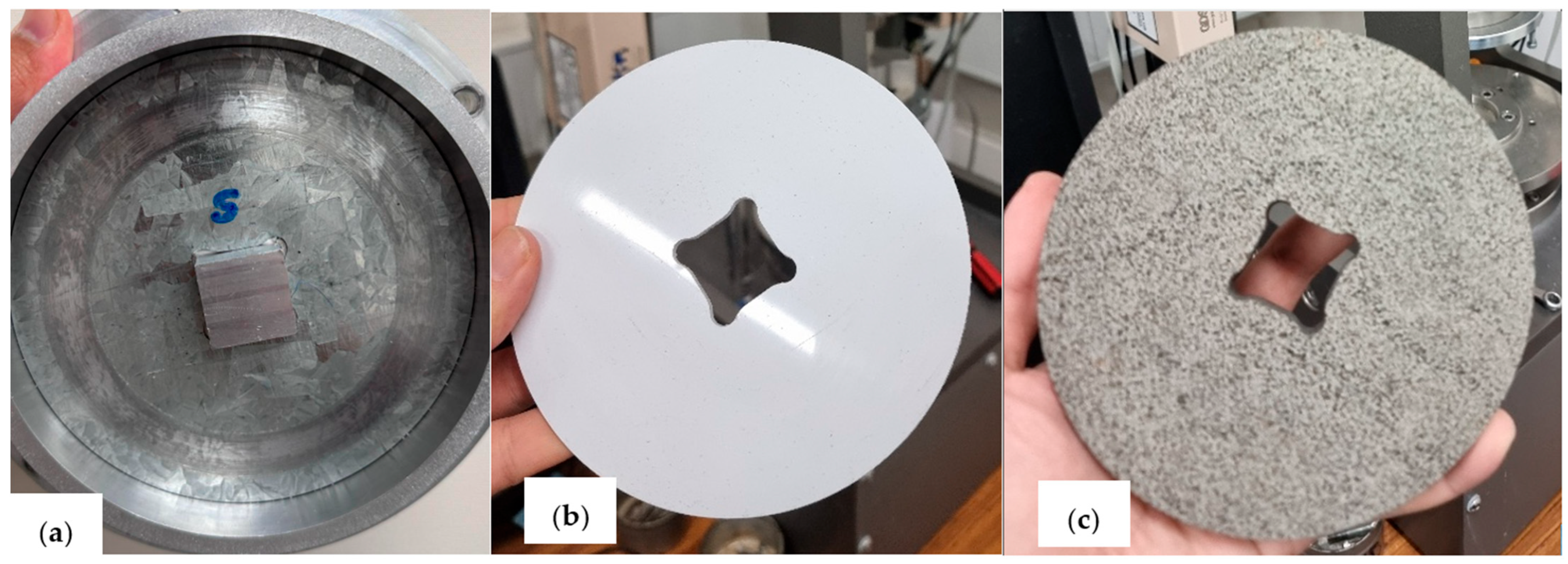
Three kinds of continuum interface materials were studied: steel, polyvinyl chloride (PVC), and natural stone (refer to Figure 3). Their surface properties were carefully characterised by total roughness (R_t) and interface hardness (HD). Roughness was measured by geometric measures of surface asperities, and reflects scaling of surface features, which relates to mechanical interlocking and friction after rolling or sliding. Hardness was measured by using indentation size techniques, which indicate the surface resistance to localised deformation or ploughing caused by soil particles. According to

Table 4. Properties of the continuous surfaces used in the study.

Material	Rt (μm)	HD
Steel	4.2	112.2
PVC	0.45	50
Stone	82.92	795

, steel had moderate roughness (~4.2 m) and hardness (~112.2 kPa); PVC had low roughness (~0.45 m) and intermediate hardness (~50 kPa); and stone exhibited a much higher roughness (~82.9 m), with hardness of ~52.2 kPa. These different types of interface properties allowed for a range of interface conditions to test the effect that surface mechanical characteristics have on soil shear behaviour.

2.2. Ring Shear Testing Procedure

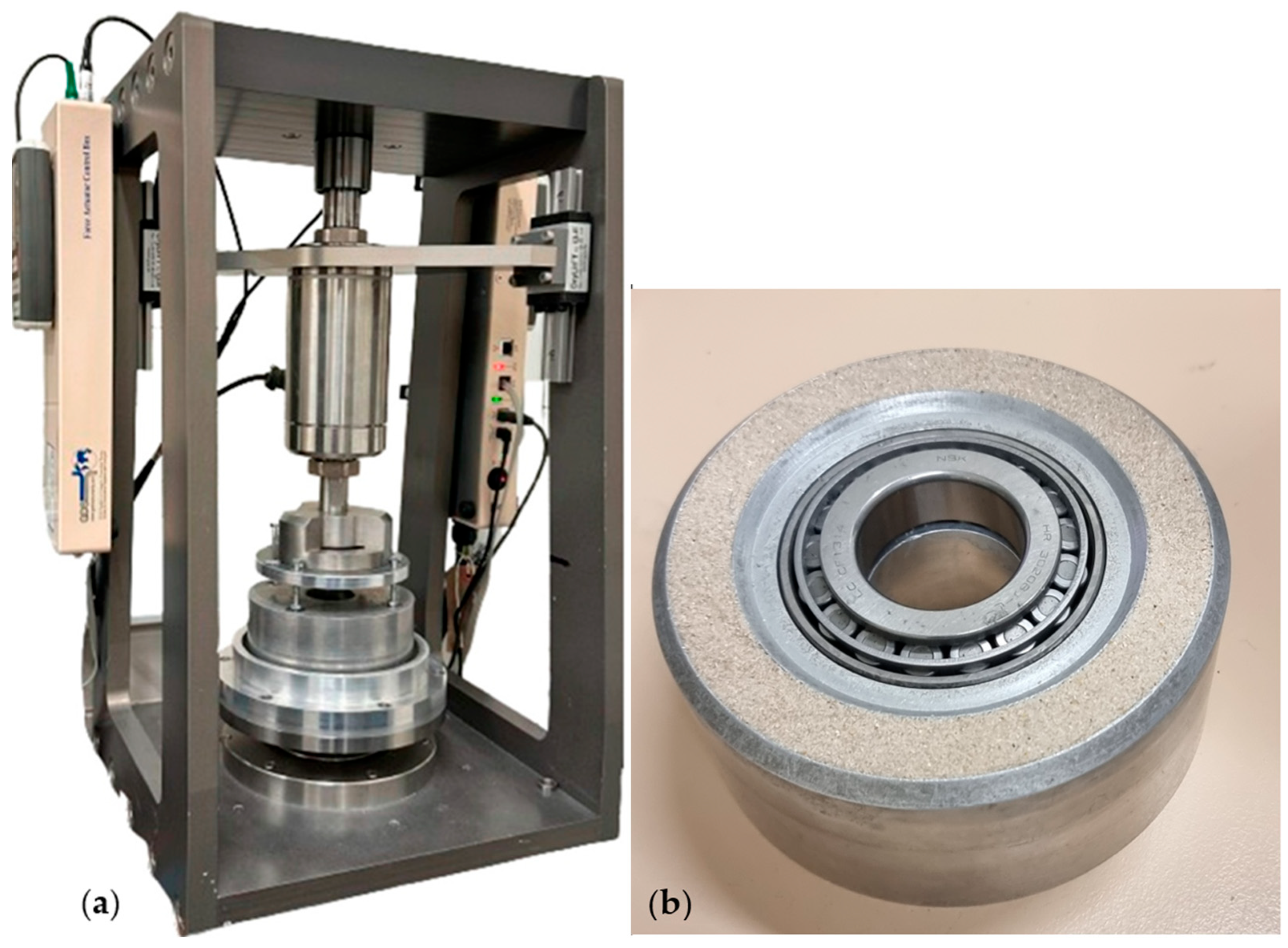
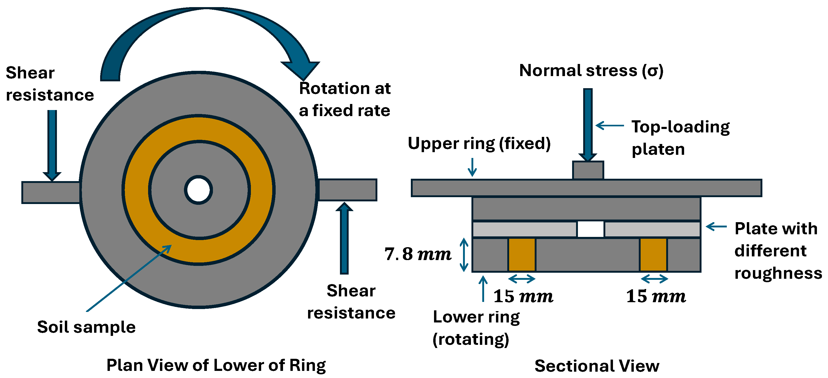
The ring shear tests were performed using a GDS ring shear apparatus (GDS Instruments Ltd., Hook, Hampshire, UK), which was subsequently modified by the authors as described herein. (refer to Figure 4). The original rotating mould was swapped out for the new mould set, which included a shearing mould and an interface plate to which continuum material samples were attached. The shearing mould had a ring-shaped channel that was approximately 7.8 mm deep and 15 mm wide to contain the sand sample while permitting a controlled shearing displacement of the soil relative to the fixed continuum plate below (refer to Figure 5).

Table 5. Specifications of the GDS ring shear apparatus used in this study.

Parameter	Specification
Manufacturer/Model	GDS Instruments—Ring Shear Apparatus (modified)
Shear box geometry	Annular ring, 15 mm width × 7.8 mm depth
Maximum normal load	Up to 1000 kPa (this study: 25, 50, 100 kPa)
Shear displacement mode	Continuous rotation (no displacement limit)
Maximum shear displacement	Unlimited (continuous shearing)
Shear rate range	0.001–10 mm/min (this study: 0.5 mm/min)
Normal stress application	Pneumatic loading system
Load measurement accuracy	±0.5% of applied load
Displacement resolution	0.001 mm

represents specifications of the GDS ring.

The selected normal stresses (25, 50, 100 kPa) correspond to approximate soil depths of 1.3, 2.6, and 5.1 m for typical sand densities of 18–20 kN/m³, which are representative of stresses acting on shallow foundations and embankments.

The ring shear setup allowed for continuous rotation, meaning peak and residual shear strengths could be evaluated while continuously subjected to shearing. In contrast to the typical direct shear test, which has displacements constraints that would yield an inaccurate residual shear strength, the ring shear apparatus allows for large relative displacements, without boundary effects to interfere, and simulates field conditions, such as slow landslides or long durations of soil–structure interactions. The shear plane is uniformly stressed, since there the design minimises the edge effect seen with a direct shear device, contributing to more representative and trustworthy interface shear strength data.

Each of the samples were tested under three normal stress states as shown (25 kPa, 50 kPa, and 100 kPa), which are likely to be representative of loads on shallow foundations/embankments. Shearing was performed at a constant rate of 0.5 mm/minute. This rate of deformation was selected to bracket quasi-static soil deformation rates per geotechnical applications. Repeated tests were performed for each combination of sand type and, the continuum surface to give confidence in the statistical robustness of each pump-type interface generated setting, which included 90 individual shear tests consisting of peak and residual shear strength tests under controlled laboratory conditions. Full density states (loose/dense) were also arranged for all samples, measured using the sand-raining method to capture how packing states influenced interface behaviour.

During the tests, shear stress and displacement were recorded continuously, allowing for the identification of the peak interface shear strength (τ_max) and residual shear strength (τ_residual), of which only the maximum shear strength was used as an output for predictive modelling efforts.

2.3. Data Processing and Parameterisation

Eight inputs were chosen to model the behaviour of interface shear strength, which incorporates the various key geometric, mechanical, and loading considerations for the soil–structure interaction response. The included inputs were (1) regularity index (RI), which describes the shape of the particles, (2) median particle size (D₅₀), which describes the representative grain size, (3) porosity (n), which describes the packing density of the soil, and (4) grading characteristics via coefficients of uniformity (C_u) and curvature (C_c). The surface feature and material properties of the continuum are described by (5) surface roughness (R_t) and (6) hardness (HD), while the (7) applied normal stress (σ_n) accounts for loading conditions. Finally, together these eight inputs portray a more comprehensive framework for modelling the interface shear response.

The eight input parameters (RI, D₅₀, n, C_u, C_c, R_t, HD, σ_n) were selected to represent key measurable properties of the soil and interface, as identified in our experimental program. While the correlation matrix indicated strong linear relationships for some variables (e.g., RI, σ_n), others with weaker direct correlations (e.g., C_u, C_c, HD) were included to capture nonlinear or interactive behaviours. Subsequent SHAP analysis confirmed that dominant variables could be distinguished while still retaining secondary parameters for improved predictive consistency.

Moisture content and cyclic loading were not considered in this study, as the focus was on establishing a controlled dry sand–interface dataset under monotonic conditions. These effects, while highly relevant to real-world performance, require separate experimental programs and are identified as future research needs (see Section 5.6).

Testing and Training Databases

The experimental dataset generated from laboratory testing was split with 80% used for training and 20% used for testing to build and validate whatever predictive models. The modelling process involved a 10-fold cross validation method during training to promote generalisability and model robustness. Data preprocessing, normalising, and noise reduction was implemented to improve numerical stability, promote algorithm convergence, and maintain sharpening of predictive capacity in the model. Statistical analysis confirmed that the dataset captured a wide variety of interface conditions across several sands and continuum types. Reliability was further confirmed through consistent elastic and plastic trends relating to descriptions in loading levels, and interface dilative/constrictive characteristics of the behaviour.

2.4. Modelling Approaches

The study was focused on developing five modelling approaches, starting with multiple linear regression as the simplest statistical model, and four models with a combination of Genetic Programming (GP) with some new and advanced machine learning methods in order to predict maximum and residual interface shear strengths.

All Genetic Programming and hybrid models were implemented in Python 3.10 using the DEAP library, supplemented with custom scripts for SHAP integration, Fourier feature augmentation, and physics-informed constraints.

2.4.1. Pure Genetic Programming (GP)

Genetic Programming (GP) was used as a symbolic regression procedure as a method to evolve mathematical expressions to link the input parameters to shear strength outputs [55,56,57]. The GP used evolutionary operators (crossover, mutation, and selection) to explore the solution space for symbolic formulas, to transform the input parameters into shear strengths [58]. This method of symbolic regression prioritises interpretability via providing explicit functional relationships, which result in insights into mechanistic explanation, which are often lost in black-box methods. In order to prevent over-fitting and maintain model simplicity consistent with engineering practice, constraint and parsimony pressure were put into place to avoid over-fitting and to preserve model simplicity.

2.4.2. Natural Gradient Boosting–GP Hybrid Method

This notion of a combination methodology proposed Natural Gradient Boosting (NGBoost), a probabilistic ensemble learning framework, with symbolic regression [59]. NGBoost first analyses the probabilistic features spatial distribution in the interface shear data, but allows for variability and uncertainty in the experimental environment to exist with the data set [60]. NGBoost is also used to help define the symbolic regression portion of the analysis, which searches for interpretable expressions that represent the expected shear strength outcomes. This two-stage modelling adds noise resistance and helps extract compact formulas that weigh accuracy and interpretability.

2.4.3. Shapley Additive Explanations–GP Hybrid-Guided Symbolic Regression

In this approach the SHAP (Shapley Additive Explanations) framework was implemented within XGBoost in order to generate a feature importance metric, allowing the researcher to have a data-driven approach for defining input parameters that are impactful to the predicted outcome [61]. In these cases, the subset of parameters with the highest impact was selected to constrain the symbolic regression search space guiding the GP to develop formulae from only the important predictors [62]. This feature-guided symbolic regression incorporated not only computational efficiency but also an element of transparency. SHAP values yielded quantifiable explanations to promote scientific justification for how soil–interface behaviour emerges.

2.4.4. Physics-Informed Neural Fourier Genetic Programming (PIN-FGP)

Physics-Informed Neural Fourier Genetic Programming (PIN-FGP) is an advanced hybrid modelling framework that integrates the symbolic equation generation capability of Genetic Programming (GP) with the spectral feature extraction of Fourier transformations and the constraint-enforcing principles of physics-informed learning. In this approach, relevant physical laws and monotonicity conditions are embedded into the GP search space, guiding the evolution of candidate models towards solutions that not only minimise prediction error but also adhere to known geotechnical behaviour (e.g., positive correlation between normal stress and shear resistance). Fourier features enhance the model’s ability to capture nonlinear, periodic, or interaction effects between variables, while the neural component improves feature representation before symbolic regression. This combination produces compact, interpretable equations that maintain high predictive accuracy, avoid unphysical trends, and remain directly applicable for engineering design and analysis.

Physics-informed constraints were incorporated by adding penalty terms to the GP fitness function. Candidate formulas that violated fundamental mechanical expectations, such as negative shear strength values or non-monotonic increases of τ_max with σ_n, were assigned higher penalty costs, guiding the evolutionary search toward physically consistent solutions.

2.4.5. Fourier Feature-Augmented Genetic Programming (FF-GP)

The Fourier Feature-Augmented Genetic Programming (FF-GP) technique allows trigonometric basis functions to be input into the symbolic regression process, enabling the FF-GP to recognise periodic and oscillatory relationships within interface shear strength data [63]. During preprocessing forms of GP modelling, the sine and cosine transformations of the input variables are used, with the same methodology adopted in Fourier series approximation [64]. This Fourier feature augmentation enhances the input space of the GP, allowing the assignment of target functions that include sinusoids within it to better account for potential underlying physical data generation processes, and is, in particular, helpful for representations/models that include micro-roughness patterns, or loads that are applied in cycles. The task of GP is to discover formulas representing interpretable mathematical relationships that combine the original selected input variables and their sinusoidal versions. The process of generating trigonometric representations is guided by pre-identified parsimony constraints so that there is little added complexity. The FF-GP approach allows for facilities to manage and balance a representation with fidelity or complexity while providing usable functional transparency, developing forms of formulas for practising engineers that illustrate both linear and cyclic dependencies within the shear resistance mechanism.

Fourier feature augmentation was adopted because soil–interface interactions often display periodic micro-scale effects arising from asperity interlocking and cyclic sliding. Trigonometric basis functions are able to approximate such oscillatory behaviours, allowing the GP to capture localised fluctuations in shear strength while still producing interpretable symbolic formulas.

2.5. Model Evaluation Metrics

The performance of the predictive models was evaluated using a number of statistical metrics: mean absolute error (MAE), root mean square error (RMSE), root mean squared logarithmic error (RMSLE), and the coefficient of determination (R²). These statistics (introduced in Equations (1)–(6)) provided a quantifiable method of evaluating accuracy across the training, testing, and 10-fold cross-validation datasets, which allowed for useful comparisons of different methods. The interpretative quality of the models was qualitatively assessed based on the complexity of the formula, and the consistency of feature relevance with the established theory of physical soil mechanics.

$$MAE={\displaystyle \frac{1}{n}}{\sum }_{i=1}^n\left|y_i-\widehat{y_i}\right|,$$

(1)

$$MSE={\displaystyle \frac{1}{n}}\sum _{i=1}^n{\left(y_i-\widehat{y_i}\right)}^2$$

(2)

$$RMSE=\sqrt{MSE}$$

(3)

$$MSLE={\displaystyle \frac{1}{n}}\sum _{i=1}^n{\left(\log \left(1+y_i\right)-\log \left(1+\widehat{y_i}\right)\right)}^2$$

(4)

$$RMSLE=\sqrt{MSLE}$$

(5)

$$R^2=1-{\displaystyle \frac{\sum _{i=1}^n{(y_i-\widehat{y_i})}^2}{\sum _{i=1}^n{(y_i-\overline{y})}^2}}$$

(6)

where:

n = total number of data samples.

$y_i$ = actual (observed) value of Factor of Safety (FOS) for the i-th sample.

$\widehat{y_i}$ = predicted value of Factor of Safety (FOS) for the i-th sample.

$\overline{y}$ = mean of actual (observed) Factor of Safety (FOS) values across all samples.

2.5.1. Model Regularisation, Complexity Control, and Validation Strategies

Since Genetic Programming (GP) can create flexible symbolic expressions, it is important to consider ways to regularise the models, assess complexity, and avoid over-fitting, especially when using a relatively more complex feature transformations (like trigonometric functions), and incorporating the probabilistic outputs of ensemble approaches. In this case, a series of regularisation principles and validation techniques were used to provide the evolved models an optimum balance of predictive power, level of complexity, and generalising ability.

2.5.2. Parsimony Pressure and Complexity Penalty

In order to constrain the GP models from producing overly complex formulas, a parsimony pressure was added to the fitness function. The parsimony pressure penalises formula size by adding a weighted cost based on the number of nodes (function and terminal symbols) represented in the expression tree. In the fitness function:

Fitness = Error_MSE + λ × Complexity_Nodes

(7)

where λ is the complexity penalty coefficient (empirically set to 0.01 after sensitivity tuning), and Complexity_Nodes represents the total number of nodes in the evolved expression. This encourages the evolutionary process to favour simpler, more interpretable formulas without compromising predictive performance.

2.5.3. Function Set Constraints

The GP search space was also restricted further by the function sets available during the evolution of symbolic expressions. For the Fourier feature-augmented model, trigonometric functions (sin, cos) were used, but were further constrained by the formula depth limitation (6 levels) to limit excessive nesting of nonlinear components, which could lead to over-fitting.

2.5.4. Early Stopping Criteria

A mechanism for early termination exists in the loop structure of GP evolution. If a model reached saturation in performance, that is, no improvement on the validation set (a dataset separate from the training data) was recorded over the course of 50 generations, then the evolution loop would terminate. This ensures that the needlessly introduced complexity does not continue to escalate beyond the point when performance is established, at which point the amount of complexity is null to performance.

2.5.5. Cross-Validation Strategy

A 10-fold cross-validation method was undertaken to guarantee that model generalisation and robustness could occur over the entire dataset. The model was subjected to a 10-fold split, producing 10 equal subset groupings of the dataset. Each iteration would use one subset as the validation (test) dataset, while the remaining nine subsets would be used as training dataset. The overall performance metrics (e.g., R², RMSE, MAE, MBE) were averaged over all folds. The out-of-sample predictive ability was assessed on a final 80–20 train–test split, with the same metrics of performance applied.

2.5.6. Leave-One-Out Cross-Validation for Outlier Panel Subsampling

A leave-one-out cross-validation (LOO-CV) methodology was employed for the purpose of determining model sensitivity to outlier samples within the panel. To account for individual high-variance samples, a leave-one-out process builds sequential nested models iteratively each time eliminating a single sample from the training dataset. LOO-CV would promote model validity aimed at producing reliable predictive estimations for samples at the higher τ_max (>50 kPa) range where it was documented that sample sparsity exists across τ_max range.

Through this multi-tiered regularisation and validation framework, the evolved GP models were constrained to produce compact, interpretable, and generalisable formulas, effectively mitigating over-fitting risks and enhancing the models’ practical applicability in diverse geotechnical scenarios.

3. Experimental Data Analysis and Preprocessing

Accurate determination of soil–structure interface shear strength involves careful experimental design, control of testing conditions, and data collection. Laboratory ring shear tests, like those used in this study, have a unique advantage in sensing the entire stress–displacement relationship, specifically large fault displacements, as the peak and residual strengths can be clearly defined. Repeatable elements of sample preparation, consistent loading rates (in this case, 0.5 mm/min), and the clear characterisation of soil and interface properties will produce reliable datasets for further modelling. For this research, 90 individual shear tests were performed across five sands and three interface materials at normal loading levels of 25, 50 and 100 kPa and hardness (HDS) ranging from 50 MPa (PVC) to 795 MPa (stone).

Figure 6 shows that τ_max is affected by the interface hardness (HD) and applied normal stress (σ_n). The measured τ_max values range from 3.0 kPa to 54.0 kPa because the highest τ_max values occurred when σ_n was approaching 100 kPa and HD was greater than 700 MPa. At lower hardness levels (e.g., HD ≈ 50 MPa), τ_max increased sharply with σ_n, wherein an average of 8.5 kPa was at σ_n = 25 kPa, and 30.2 kPa was at σ_n = 100 kPa, which is greater than a 250% increase in τ_max. For high-hardness interfaces (HD > 700 MPa), τ_max increased from 22.5 kPa at σ_n = 25 kPa, to 52.0 kPa at σ_n = 100 kPa, with a smaller relative increase (~130%) since the stiff interface already provided a fairly high baseline resistance. These patterns are consistent with our broader understanding cutaneous fouling τ_max is derived from frictional sliding, particle interlocking, and micro-asperity deformation, each moderated differently by normal load and interface stiffness. Higher σ_n mobilises example more particle, surface contact and engagement of asperities for friction, while higher HD acts to limit asperity crushing and plastic deformation to initiate and maintain larger effective friction angles at the interface.

Figure 7 demonstrates, then, how both Rt and RI exhibited a marked effect on the maximum interface shear strength (τ_max), including a clear nonlinear relationship. Overall, τ_max increased with increased R_t; it correlated well with mechanical interlocking, especially in the intermediate RI cases (0.50–0.60). τ_max tended to remain below 18 kPa for R_t < 10 µm across all RI. τ_max exceeded 30 kPa when Rt was greater than 60 µm; discreet observations ranged as high as above 50 kPa. The shape of the particles also had a clear effect; τ_max values were higher for lower RI (irregular particles), and for the same R_t, this could be due to better interlocking. Similarly, at very high RI (>0.65), the benefits of increasing R_t began to drop off, potentially indicating that smoother particles were not able to mobilise the full ability of rougher interfaces; thus, roughness can be thought of not just as surface roughness but as one aspect of particle and interface characteristics. All of this is consistent with soil–structure interaction theory, and broad ratings of soil property relations to gravel strength performed in previous studies (e.g., Uesugi and Kishida [2]; Dove and Frost [3]). For instance, soil–structure interaction theory explains that rough surfaces, like angular particles, can increase the resistance to shear failure by mechanical interlocking. Conversely, smooth particles were shown to reduce the ability for engagement with roughness (asperities). The curvature of the surface plot probably reflects the complementary relationship between micro-scale contact mechanics and macro-scale stress.

The sensitivity of τ_max to RI and R_t agrees with multiscale findings that irregular particles generate local stress concentrations and interlocking effects, while rounded particles promote more uniform load transfer [60].

Table 6. Statistical information of the training database.

Variable	Observations	Minimum	Maximum	Mean	Std. Deviation
τmax (kPa)	72	3.000	52.500	22.448	13.794
RI (-)	72	0.370	0.715	0.490	0.139
D50 (mm)	72	0.510	1.770	1.084	0.594
γd (g/cm3)	72	1.570	2.750	1.900	0.282
Cu (-)	72	1.200	6.200	2.482	2.010
Cc (-)	72	0.960	1.310	1.054	0.139
Rt (µm)	72	0.500	82.920	33.774	33.219
HD (N/mm2)	72	50.000	795.000	300.100	331.610
σn (kPa)	72	25.000	100.000	56.597	30.832

shows the summary statistics of the training dataset with 72 cases for each variable. The maximum shear strength (τ_max) varies from 3.0 to 52.5 kPa with a mean value of 22.448 kPa and a standard deviation of 13.794 kPa indicating large variation among cases of record. The regularity index (RI) varied moderately from 0.370 to 0.715 with an average of 0.490. The particle size distribution value of D₅₀ ranged from 0.510 mm to 1.770 mm with an average of 1.084 mm, suggesting a range of gradations. Similarly, the dry unit weight (γ_d) ranged from 1.570 to 2.750 t/m³ with a mean of 1.900 t/m³, indicating diversity in soil compaction. The coefficients of uniformity (C_u) and curvature (C_c) both showed some level of variability, especially C_u, which had a high standard deviation (2.01), suggesting a wide variety of particle size distributions. Other variables, such as total roughness (R_t), hardness (HD), and normal stress (σ_n), exhibited high dispersion with R_t and HD, with very high standard deviations closely around their mean values. Such spreading among variables indicate a diversity of material and test conditions for the training dataset.

Table 7. Statistical information of the testing database.

Variable	Observations	Minimum	Maximum	Mean	Std. Deviation
τmax (kPa)	18	5.300	54.000	27.922	16.844
RI (-)	18	0.370	0.715	0.570	0.137
D50 (mm)	18	0.510	1.770	0.803	0.533
γd (g/cm3)	18	1.660	2.750	2.062	0.376
Cu (-)	18	1.200	6.200	1.811	1.600
Cc (-)	18	0.960	1.310	1.006	0.111
Rt (µm)	18	5.000	82.920	42.853	37.066
HD (N/mm2)	18	50.000	795.000	394.933	368.945
σn (kPa)	18	25.000	100.000	65.278	33.364

summarises the statistical summary for the testing dataset, which contains 18 observations. In comparison to the training sample, τ_max in the testing samples has a higher mean value (27.922 kPa) and a larger range (5.3 to 54.0 kPa). D₅₀ and C_u have lower mean values (0.803 mm and 1.811) than the training samples, which indicates that the testing samples contained finer particles and less uniformly gradated soils. The dry unit weight (γ_d) also had a higher mean (2.062 t/m³), which was representative of more compacted soils. Each of the variables, R_t and HD, have higher average values, and higher variability, especially for HD, which has a range of 50–795 mm and a standard deviation of 368.945 mm. The mean normal stress (σ_n) is slightly higher in the testing samples (65.278 kPa), indicating that the testing samples have much higher stress conditions than the training dataset.

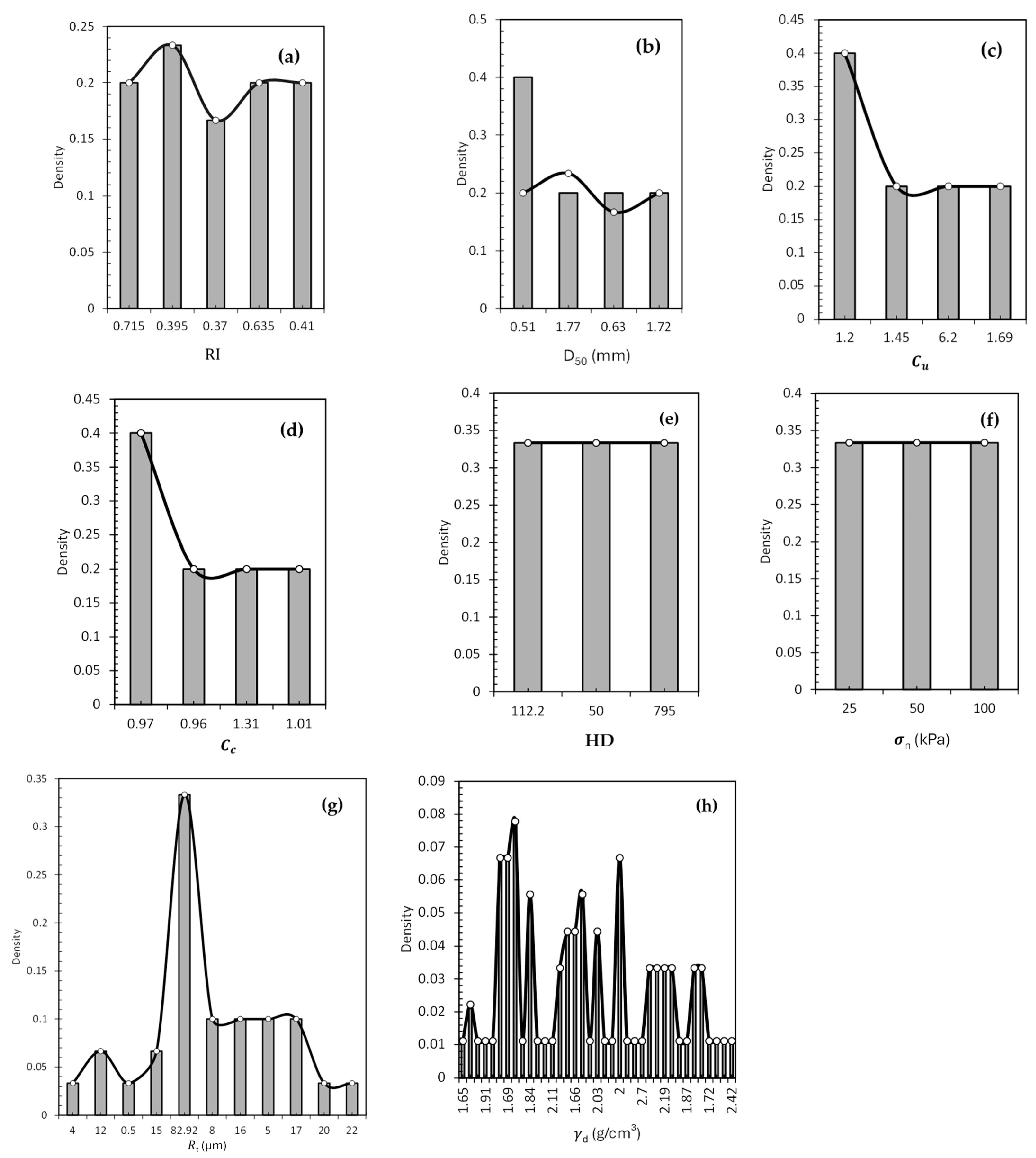
Figure 8 presents the normalised distribution of the main variables in the database, as well as their associated statistical spread and frequency distributions. The regularity index (RI) has a fairly uniform distribution, with minor peaks near 0.395 and 0.635, throughout the range of 0.370 to 0.715. This indicates that the database has a balance of dense and loose soils assembled for testing. The D₅₀ variable has a rightward skewed distribution, with the majority of samples collected in the finer particle size of 0.51 mm. The dry unit weight (γ_d) demonstrates a very scattered distribution relative to the range of 1.57 to 2.75 t/m³, without a dominant peak showing a diverse compaction state per sample. The distribution of the coefficient of uniformity (C_u) and the coefficient of curvature (C_c) are also skewed, with both having prominent peaks at lower values (C_u~1.2, C_c~0.96), indicating that well-graded soils predominated over uniformity. The total roughness (Rt) has a sharp peak at approximately 83 kPa, implying that a dominant cluster of samples had tensile strength around this value, and a nearly unlimited number of samples that demonstrated total roughness lower than this peak. The hardness (HD) and normal stress (σ_n) are uniformly distributed with these parameters, indicating that controlled and balanced testing conditions were applied.

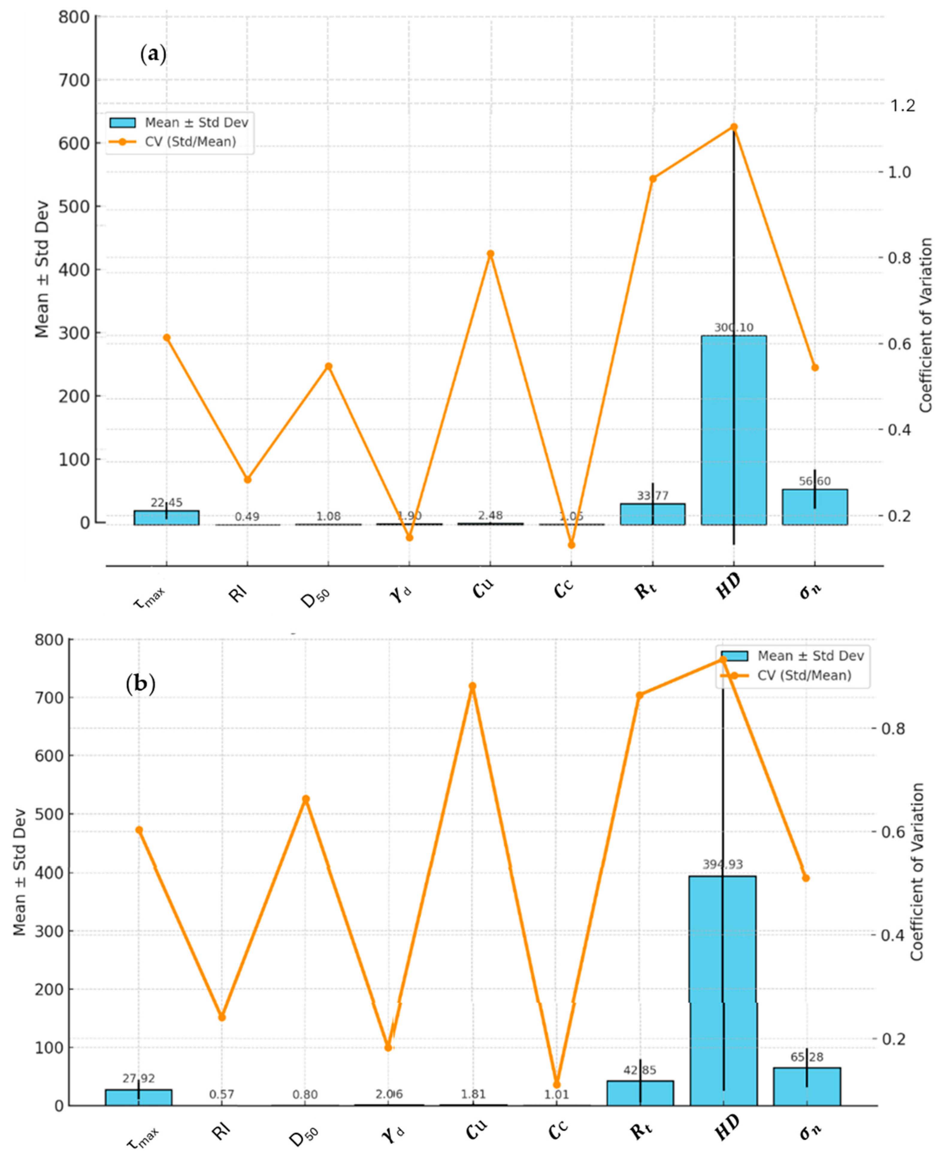
Figure 9 summarise the mean, standard deviation (Mean ± Std Dev), and coefficient of variation (CV) for the training and testing datasets. In the training dataset (Figure 9a), τ_max had a mean of 22.45 kPa with a CV of about 0.61, indicating that shear strength had moderate variability, meaning this parameter was likely important in the model. Some variables, such as RI and D₅₀, had CVs that were relatively low (0.28 and 0.55), indicating relative consistency in regularity index and grading of particle sizes. C_u and R_t had a higher variability, with CVs greater than 0.80, and HD had the highest CV (greater than 1.0), indicating that hardness measurements had extreme dispersion. The testing dataset (Figure 9) had an only slightly larger mean τ_max of 27.92 kPa and a CV of 0.60. RI and D₅₀ had similarly low variability (CVs of 0.24 and 0.66), but C_u, R_t, and HD had significant dispersion in τ_max measurements in accordance with training dataset CV measurements, especially HD with a CV of about 0.93.

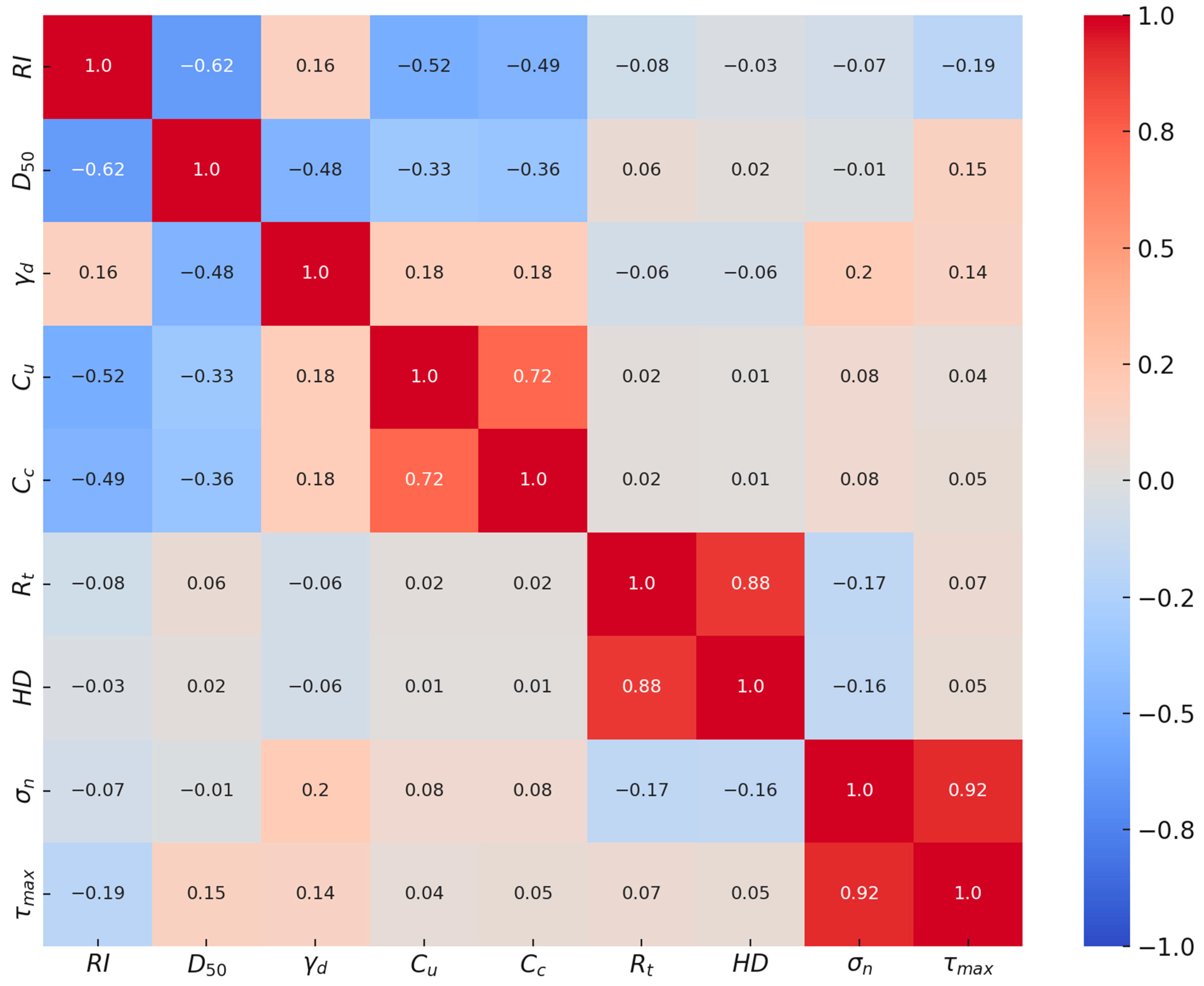
Figure 10 demonstrates a correlation matrix of all the variables identifying the strength and direction of linear relationships among them. There exists higher positive correlation (r = 0.92) between normal stress (σ_n) and maximum shear strength (τ_max). This suggests that τ_max experiences a proportional rise in stress applied, which is consistent with shear strength behaviour. In addition, total roughness (R_t) and hardness (HD) demonstrate very high correlation (r = 0.88). Therefore, it is suggested that Rt and HD as parameters are directly related, likely due to test setup limitations. Moderate positive correlations exist between C_u and C_c (r = 0.72), respectively, indicating that they have some dependence on soil gradation characteristics. When reviewing RI, a negative correlation exists with D₅₀ (r = −0.62) and C_u (r = −0.52), respectively, indicating that an increase in regularity index increased the form of finer particle size and less uniform gradation.

Although C_u, C_c, R_t, and HD exhibited weak linear correlations with τ_max, this does not imply irrelevance. The correlation matrix captures only direct linear relationships, whereas these parameters mainly influence τ_max through nonlinear interactions. For instance, R_t and HD are strongly correlated with each other (r ≈ 0.88), which reduces their apparent marginal impact, while C_u and C_c have skewed distributions that suppress linear sensitivity. Retaining these parameters was therefore important, and our GP-based and SHAP-guided analyses confirmed that they contribute to improved predictive accuracy and physical consistency by capturing these nonlinear and coupled effects.

4. Predictive Modelling Results

In this section, the predictive performance of different modelling approaches that were developed to predict maximum interface shear strength (τ_max) from experimental input parameters are presented and compared. This study used both standard statistical modelling techniques and advanced hybrid symbolic regression methods to explore a balance between predictive accuracy and model interpretability. The experiments were conducted using roughly 100 samples and were separated into a training set of roughly 80 cases and a test set of roughly 20 cases, allowing each model to be assessed for generalisability. Model performances were compared based on predicted versus observed τ_max values, with some emphasis on accuracy, trends, and modelling methods ability to represent obscured patterns in the data.

4.1. Multiple Linear Regression (MLR)

The first modelling approach utilised was the multiple linear regression (MLR) method, which served as a point of reference for the more advanced techniques. The training and testing dataset of the predicted versus observed τ_max plot is presented in Figure 11. The dataset consists of 92 samples, where 74 samples were used for training and 18 samples were used for testing. The ideal 1:1 linear correlation is illustrated in Figure 11.

The MLR model properly encapsulates the overall linear relationship between input variables and τ_max inferred from the training dataset, as shown by the close grouping of training data along the 1:1 line. However, upon applying the MLR model to the testing dataset (where the τ_max values range from 6.6 kPa to 54 kPa), the model exhibits moderate variability, especially at higher τ_max values. It can be seen that an observed τ_max of 45.5 kPa was under-estimated down to 38.72 kPa, and that an observed value of 25.78 kPa was over-estimated up to 37.32 kPa. The MLR model simply does not allow for full capture of the nonlinearities and interactions that are present in interface shear behaviour. Still, the MLR model provides a solid primary relationship as a baseline to assess how well the hybrid symbolic regression methods perform in the following sections.

Equation (8) shows the proposed formula to predict maximum shear strength based on the MLR method:

τ_max = −65.98 − 65.90 × RI − 10.38 × D₅₀ − 3.20 × γ_d − 12.91 × C_u + 135.40 × C_c + 0.22 × R_t − 0.01 × HD + 0.43 × σ_n

(8)

Figure A1 gives a precise statistical representation of the predictive ability of the multiple linear regression (MLR) model when predicting maximum interface shear strength (τ_max). Figure A1a displays the distribution of relative errors based on the MLR predictions for all the data available, 92 samples total. The majority of relative errors exist inside the interval (−0.25 to +0.25), with the relative error distribution peaking around 0, indicating that as a rule MLR predicts τ_max values with small variations from the actual predicted values. Approximately 78% of the samples (72 out of 92) have relative errors in the −0.30 to +0.20 range as well, which demonstrates acceptable prediction accuracy. There is a small left-skew, indicating a slight typical systematic under-estimation tendency. Very extreme errors beyond (±0.5) are rare, less than 5% of the cases, which indicates the model offers reliable prediction stability of error dispersion.

The scatter plot of observed τ_max vs. MLR-predicted τ_max is shown in Figure A1b with marginal histograms and density plots. The Pearson statistic shows a strong relationship with a correlation coefficient of 0.9582. This indicates that there is a strong linear relationship between the model’s predictions and the actual values measured through laboratory testing, as the regression line tracks very closely alongside the ideal 1:1 line with most data points within proximity. Its positive relationship means predicted and observed values will move in the same direction (if predicted τ_max values increase, then observed values will increase almost in sync). The range of observed τ_max values was 3 kPa to 54 kPa and we can see when looking at the marginal histograms that the vast majority of data points occurred reasonably uniform across this range, with only slight clusters of densities observed. Some dispersion is observed at the max τ_max range (above 40 kPa), but generally the fit of predicted values remained stable into both the lower and mid-ranges.

Figure A1c presents a frequency histogram of actual vs. predicted τ_max values, separated for training and testing datasets. In the training dataset (74 samples), predicted τ_max values and actual τ_max values align closely together, particularly in the τ_max intervals of 10–30 kPa where frequencies are higher. In the testing dataset (18 samples), the observed τ_max values are approximately evenly dispersed, while predicted τ_max values follow a similar distribution trend, with a gradual trend of under-predicting τ_max values in higher τ_max bins (e.g., 45–50 kPa) being noted. The predicted frequencies are within +/− 2 counts of the actual frequencies in most bins, adequately capturing the global distribution of τ_max even though the MLR model is, from a modelling perspective, a linear simplification of the actual and predicted behaviour.

Spatial Surface and Error Distribution Analysis for MLR

While global evaluation metrics such as the Pearson correlation coefficient of 0.9582 and relative error histograms provide relationships indicating the predictive capabilities of the MLR model, they do not illustrate the relationships the model represents across portions of the input feature space. As τ_max can exhibit complex local variations driven by many interacting parameters, it is useful to examine the spatial distribution of both the predictions and errors. To illustrate this aspect of the feature space, a two-dimensional feature space consisting of normalised values of F1 and F2 (two dominant input variables established during prior feature importance analysis) was constructed, and the model outputs were also displayed in a manner that the predicted and real τ_max surfaces in a three-dimensional representation can be compared to assess topological similarities and differences between the actual and predicted model outputs.

Figure A2a provides a surface comparison between MLR-predicted τ_max values and actual measured τ_max values, within the feature domain of which F1 and F2 values range from 0.0 to 1.0. Both surfaces exhibit the same peak patterns, exhibiting τ_max values as high as around 40 kPa. However, where the F1 interval is from 0.5 to 0.7 and where the F2 interval is from 0.3 to 0.6, there are notable estimation inaccuracies in the predicted surface, which for the stated intervals over-estimated up to 5 kPa in relation to actual values. Meanwhile, regions where the F1 value is much less than the actual surface τ_max values (where F2 values are less than 0.2), predicted τ_max values are −3 to −4 kPa less than the actual values, where it again shows sharper gradients in the actual τ_max surface that the MLR model is not able to predict accurately.

Figure A2b shows the signed error distribution (predicted—actual) with over-estimations coloured red, and under-estimations coloured blue. It also overlays the predicted τ_max surface in a wireframe format. Signed errors mostly range from −3.2 kPa to + 3.4 kPa, and does not show extreme values of the signed error in localised predictions, thus confirming the MLR model does not significantly deviate. The large positive errors are located near F1 ≈ 0.6 and F2 ≈ 0.4, which corresponds to areas where the predicted surface shows clear artificial peaks. Conversely, large negative errors locate in areas where F2 > 0.7, with the model consistently under-predicting τ_max values by roughly 2.5 to 3 kPa

4.2. NGBoost–GP Hybrid Method Results

The hybrid method is created called NGBoost–GP, which implements symbolic regression using NGBoost with GP, to improve the predictive skill and produce models robust to noise. The NGBoost–GP hybrid search method employs NGBoost’s probabilistic ensemble learning capabilities to model the various feature distributions/covariance and variability of the data before carrying out the symbolic regression. By adding the probabilistic information from NGBoost into the search space of GP, the NGBoost–GP hybrid method produced a number of compact and interpretable formulas, which all achieved good predictive power despite the underlying uncertainty in the data (Figure 12). The hybrid model was trained on the 74 samples (80% of the dataset) and tested on the other 18 samples (20% of the original dataset) to appropriately estimate its predictive performance and generalisability.

Figure 12 shows the predicted versus observed τ_max plot for the NGBoost–GP hybrid method. The solid line indicates the ideal 1:1 line of correlation, while the dashed line indicates the regression fit of the predicted values, combined with a 95% confidence interval. The model is aligned with the ideal line well across the τ_max range from 3 kPa to 54 kPa. Approximately 90% of the samples in the training dataset were predicted within ±2 kPa of the actual τ_max values, demonstrating the ability of this model to generalise patterns learned from the training data, without over-fitting.

The test dataset reinforces the model’s robustness with a prediction error consistently within ±2.5 kPa. For example, a test sample with an observed τ_max of 42.5 kPa has a prediction of 40.8 kPa, giving a small under-prediction of −1.7 kPa, whereas a sample with an observed τ_max of 25.78 kPa is over-predicted by 27.3 kPa with a positive +1.5 kPa error. The performance of the model using the NGBoost–GP Hybrid Method is much more precise than the baseline MLR model, which had larger errors up to ±5 kPa, showing that the NGBoost–GP hybrid method performs much better with respect to prediction accuracy, especially in higher τ_max with greater variability.

The regression fit line is very close to the 1:1 line with no significant bias present across the dataset. The NGBoost model indicates the probabilistic relations of feature interactions, which captures uncertainty and overlaps with the evolved GP symbolic formula model, which has flexibility, making fit representations appropriately even for complex situations such as interface shear strength.

Equation (9) shows the proposed formula to predict maximum shear strength based on the NGBoost–GP method. All inputs and the output must be linearly normalised (from 0 to 1) before using them in the equation.

τ_max = (r₁⁴ × (RI − γ_d)² × ((RI + γ_d) × (R_t − σ_n) + R_t − 3 × γ_d) + r₁ − (γ_d + r₁) × (C_u − C_c) × (γ_d + D₅₀ − HD²)) × ((R_t − HD) × (R_t − RI) × (r₂ + 2 × σ_n − RI) + σ_n + r₂⁴ × (D₅₀ + R_t + γ_d² − γ_d × σ_n))

(9)

where r₁ and r₂ are constant and equal to 0.673 and 0.6467.

Figure A3 provides a detailed statistical evaluation of the NGBoost–GP hybrid model analytically in terms of predictive accuracy and error distribution estimating maximum interface shear strength (τ_max).

Figure A3a provides a profile of the relative error distribution from NGBoost–GP predictions across the total of 92 samples. The histogram indicates that approximately 80% of the samples have relative errors within the interval of −0.20 to +0.20, peaked around 0 indicating that the model produces highly accurate predictions in general. Compared to the MLR model results, once again including the sample outlier, the NGBoost–GP model has significantly reduced error dispersal, as the MLR model had many relative errors in excess of ±0.50. Apart from a few outliers, even if they are significant, the few outliers indicated as showing errors beyond ±0.40 confirm the NGBoost-informed symbolic regression process addressed the data variability adequately.

Figure A3b shows the scatterplot of observed τ_max versus NGBoost–GP-predicted τ_max with marginal histograms and kernel density estimates. The Pearson correlation coefficient (r = 0.9783), indicates a strong linear relationship between observed and predicted values, and exceeds the strength of correlation in the MLR model (r = 0.9582). The regression line shown in the plot appears to closely follow the 1:1 correlation line across all values of τ_max, with the greatest correspondence noted between τ_max values of 10 kPa to 50 kPa, with only small deviations as noted on the scatterplot. The marginal histograms illustrate the balanced distribution of τ_max values used within the complete data set, with the predicted density following a similar curve to the observed distribution confirming that the model reasonably predicts greater or lesser τ_max values.

Figure A3c displays the frequency distributions of predicted versus actual τ_max values for training and test datasets. The shared histogram displays indicate that NGBoost–GP predictions are aligned closely with actual τ_max distributions for every τ_max interval. For the 10–30 kPa interval, the predicted frequencies for the training and testing data are almost equal to the actual frequencies, meaning there was a maximum difference of 1–2 counts per bin. For higher τ_max (40–50 kPa), the NGBoost–GP predictions tracked the distribution trend for the actual τ_max data well, whereas the predicted maximums for the MLR model were considerably lower than the training values for this interval. This histogram comparison exemplifies NGBoost–GP’s ability to maintain the alignment in the distribution for both training and unseen testing data.

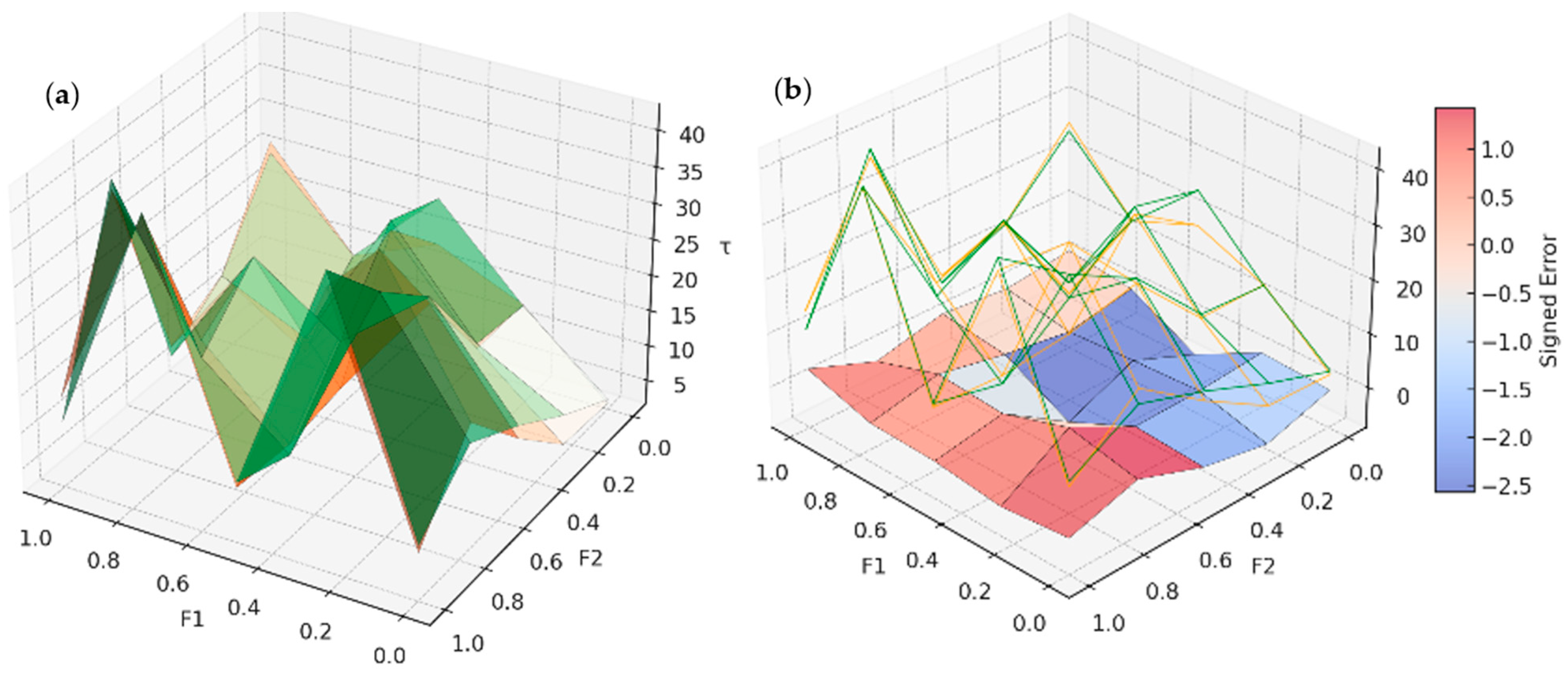
Spatial Surface and Error Distribution Analysis for NGBoost–GP

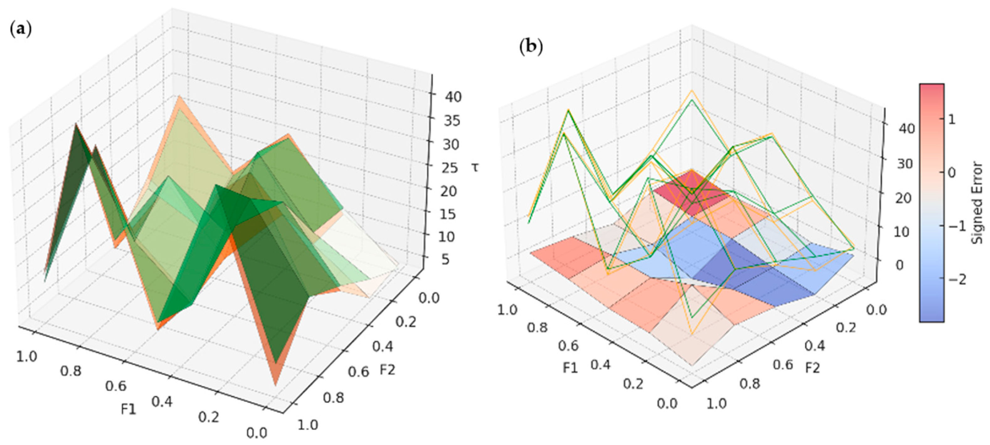
To further evaluate the strength of the NGBoost–GP model in capturing the spatial behaviour of interface shear strength (τ_max), 3D surface and error distributions were derived across the normalised feature space made up of F1 and F2. Unlike MLR, which has constraints of linearity, the NGBoost–GP model evolves its mathematical expressions in an adaptive way that allows for potential flexibility in aggregating complex features as they relate to τ_max.

Figure A4a compares the NGBoost–GP-predicted τ_max surface with the measured τ_max surface. The two surfaces show a considerable amount of similarity in topography, and in areas where τ_max is maximised at 40 kPa (or close). In comparison to MLR, NGBoost–GP shows a better fit to the higher resolution, real surface in part on the intervals between F1 = 0.3 to 0.7 and F2 = 0.2 to 0.6. The localised over-prediction in MLR is also reduced relative to the NGBoost–GP surface; NGBoost–GP surface maintains dynamic movement across midrange feature values but follows the contours of the actual surface closely. There continues to be minor differences on the boundaries (F1 < 0.2 or F2 > 0.8), but overall, the size of the difference is visibly less than for MLR.

Figure A4b shows an overlay of the predicted τ_max surface and signed error distribution (predicted—actual) for the NGBoost–GP model. The signed errors now lie within a much tighter band of −2.5 kPa to +1.5 kPa, which indicates a strong reduction in error amplitude when compared to the MLR model, where errors resulted in maximums of up to ±3.4 kPa. The regions of largest positive errors (over-predictions), were near F1 ≈ 0.2 and F2 ≈ 0.6, and had smaller length scales; while the under-predictions (negative errors) occurred when F2 > 0.7, but even then the error magnitudes were below ±2 kPa, indicating the improved performance of the NGBoost–GP model. The error surface is smoother and shows none of the steep error gradients caricatures of the MLR plots, suggesting NGBoost–GP is more flexible to incorporate nonlinearity and interactions observed in the data.

4.3. SHAP–GP Hybrid Method Results

A hybrid technique, called SHAP–GP, was created by combining Shapley Additive Explanations (SHAP) with Genetic Programming to enhance predictive performance and interpretability. Extraction of input variable importance via SHAP analysis allows for the appropriate selection of initial populations during symbolic regression search, since important parameters affect τ_max the most. This act of selecting parameters based on importance reduces the noise, requires fewer calculations, and increases stability of the formulas created through this evolution. The model was generated from training on 74 samples (80% of total dataset) and validation on 18 samples (20%) to test generalisation ability.

Figure 13 presents the SHAP–GP-predicted versus observed τ_max plot. The solid line represents the ideal 1:1 correlation. The dashed lines represent regression fits for the training and testing datasets. The 95% confidence interval is represented by the shaded area. The SHAP–GP-predicted values are close to the ideal line across the range of τ_max (3–54 kPa) with approximately 88% of the training samples being predicted to within ±2 kPa of the measured value. With the testing set, the prediction errors were generally within ±2.0 kPa, for example a test case with observed τ_max of 42.5 kPa was predicted at 41.3 kPa (ER = −1.2 kPa) and a test case with τ_max of 25.78 kPa was predicted at 26.9 kPa (ER = +1.1 kPa). The results suggest that a decisive step forward was made in predictions accuracy as the baseline MLR model may have errors up to ±5 kPa, especially for the higher τ_max values.

Equation (10) shows the proposed formula to predict maximum shear strength based on the SHAP–GP method. All inputs and the output must be linearly normalised (from 0 to 1) before using them for the equation.

τ_max = (r₁ − C_u × RI × (C_u − σ_n) + (2 × γ_d − R_t + r₁) × 2 × γ_d × (C_c − C_u))² × (((r₁ + r₂) × HD × γ_d + r₁ − RI × σ_n) × (σ_n × RI + r₂) × (σ_n × D₅₀ − HD + r₁) + R_t + (R_t − HD) × (D₅₀ − RI) + 2 × σ_n)

(10)

where r₁ and r₂ are constant and equal to 0.528 and 0.748.

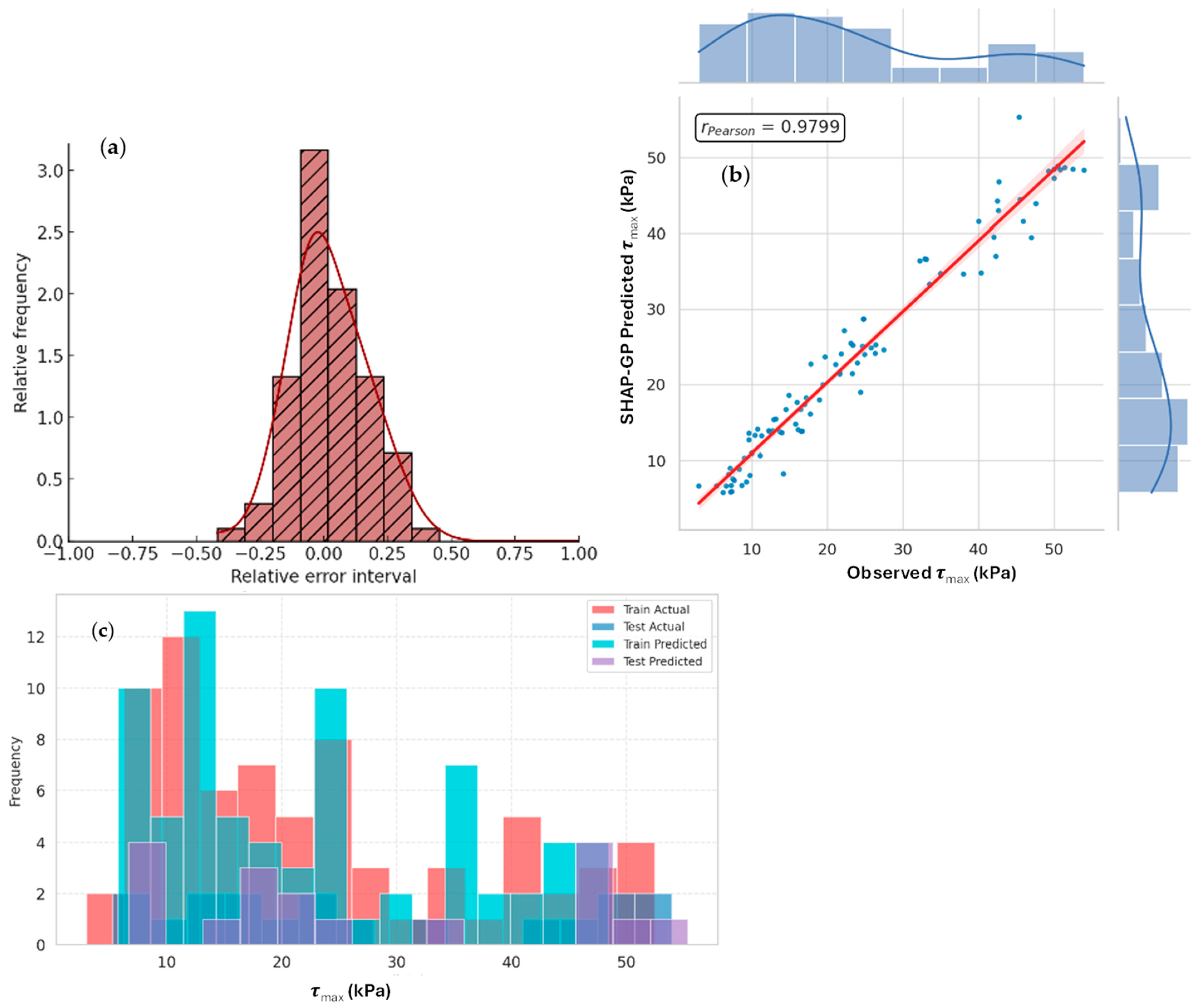
The results in Figure A5 presented provide a thorough evaluation of SHAP–GP for maximum interface shear strength prediction, specifically the distribution of errors, correlation accuracy, and distribution alignment.

Figure A5a provides the distributed relative error of predictions generated by SHAP–GP across the 92-sample dataset. The histogram provides the relative error data indicating about 85% of the samples between −0.20 to +0.20 relative error interval; the mode of frequency is near 0, which implies the system has no significant bias. Also, although the error distribution is slightly right-skewed, showing the tendency to slightly over-estimate some predictions, SHAP–GP has more tightly grouped prediction errors compared to NGBoost–GP. For SHAP–GP, there are relatively few predictions measured in the error interval above +0.30 and there were almost no outliers, predictions higher than or lower than ±0.50. This suggests that the elimination of noise based on SHAP-guided feature selection provided the Genetic Programming process an opportunity to evolve better predictive formulas.

Figure A5b presents the scatterplot for the observed τ_max versus SHAP–GP-predicted τ_max values accompanied by marginal histograms and kernel density plots. The model achieved a Pearson correlation coefficient (r = 0.9799), indicating very strong linear association between the predicted and observed values. The regression fit line is closely aligned with the 1:1 ideal line, particularly in the τ_max interval 10–50 kPa, beyond which the predicted values differed from the observed values by almost always negligible amounts. The marginal histograms further confirm SHAP–GP is maintaining the distributional aspect of the actual τ_max values as both predicted and observed values density peaks and spread are fairly closely matched.

Figure A5c presents a histogram comparison of actual τ_max and predicted τ_max values form the training and testing data sets. Overall, the SHAP–GP exhibits very good distributional alignment, as its predicted frequencies closely track the frequencies of actual values across all τ_max intervals. In the 10–30 kPa interval, the predicted frequencies are never more than 1 count different per bin compared with the actual values. In the higher τ_max interval (40–50 kPa), the model is maintaining fairly closely aligned frequencies, and exhibited a large improvement over the MLR model, which showed much larger discrepancies in those regions. In light of NGBoost–GP, it can also be seen that SHAP–GP exhibited better alignment in the testing data set, indicating better generalisation capacity probably spurred by SHAP-derived variable together at nonlinear combinations.

Spatial Surface and Error Distribution Analysis for SHAP–GP

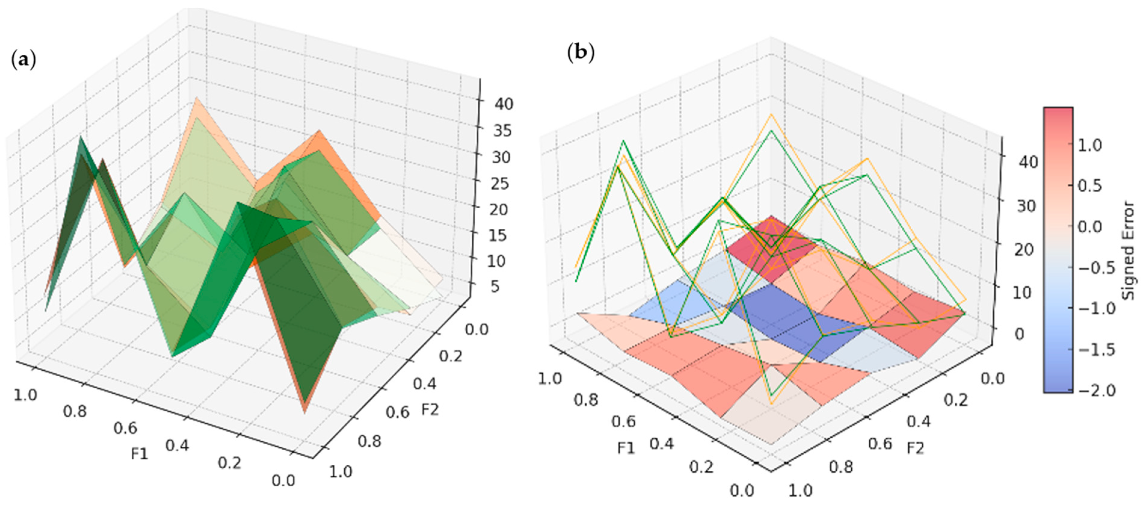
In order to assess the role of deeper evolutionary iterations or improved feature interactions within Genetic Programming, the SHAP–GP model was subsequently reviewed with 3D surface plots and signed error representations. The functional role of SHAP–GP was to optimise the (symbolic) expressions produced by NGBoost–GP, with the goal of tracking micro-patterns that exist in the interface shear strength data during areas of nonlinear behaviour.

Figure A6a presents a comparison of the τ_max surface predicted by SHAP–GP and the actual τ_max surface recorded (orange surface), across the normalised feature space of F1 and F2 (0.0 to 1.0). The SHAP–GP surface shows increasingly improved adherence to the same contours of the actual surface, compared to MLR and NGBoost–GP, particularly as τ_max exceeds 30 kPa. The degree of surface matching is substantially improved aside from the delta of F1 between 0.4 and 0.7 and F2 0.3 to 0.6, compared with the previous models that consistently over- or under-estimated τ_max. The predictive surfaces remained smooth and continuous, indicating that SHAP–GP succeeded in reducing localised prediction volatility; however, it maintained a strong connection to the overall data trends.

Figure A6b shows the signed error distribution (predicted—actual) for SHAP–GP, with a wireframe of the predicted τ_max values overlaid. The error surface has much less range of signed errors, constrained from a −2.0 kPa to a +1.2 kPa, indicating closer estimates of the errors than NGBoost–GP, which had signed errors from −2.5 kPa to +1.5 kPa, and MLR, with signed errors near ±3.4 kPa. The notable over-estimates are where F1 ≈ 0.3 and F2 ≈ 0.5 lie on the error surface; in this area the highest error does not reach further than +1.2 kPa. In contrast, under-estimates for SHAP–GP are concentrated on F2 > 0.7, where the highest errors sat around −2.0 kPa. Relative to the NGBoost–GP model, the SHAP–GP model has an even distribution of errors across the feature space, suggesting greater stability in the predictive behaviour of the evolved formula.

4.4. Physics-Informed Neural Fourier Genetic Programming (PIN-FGP) Results

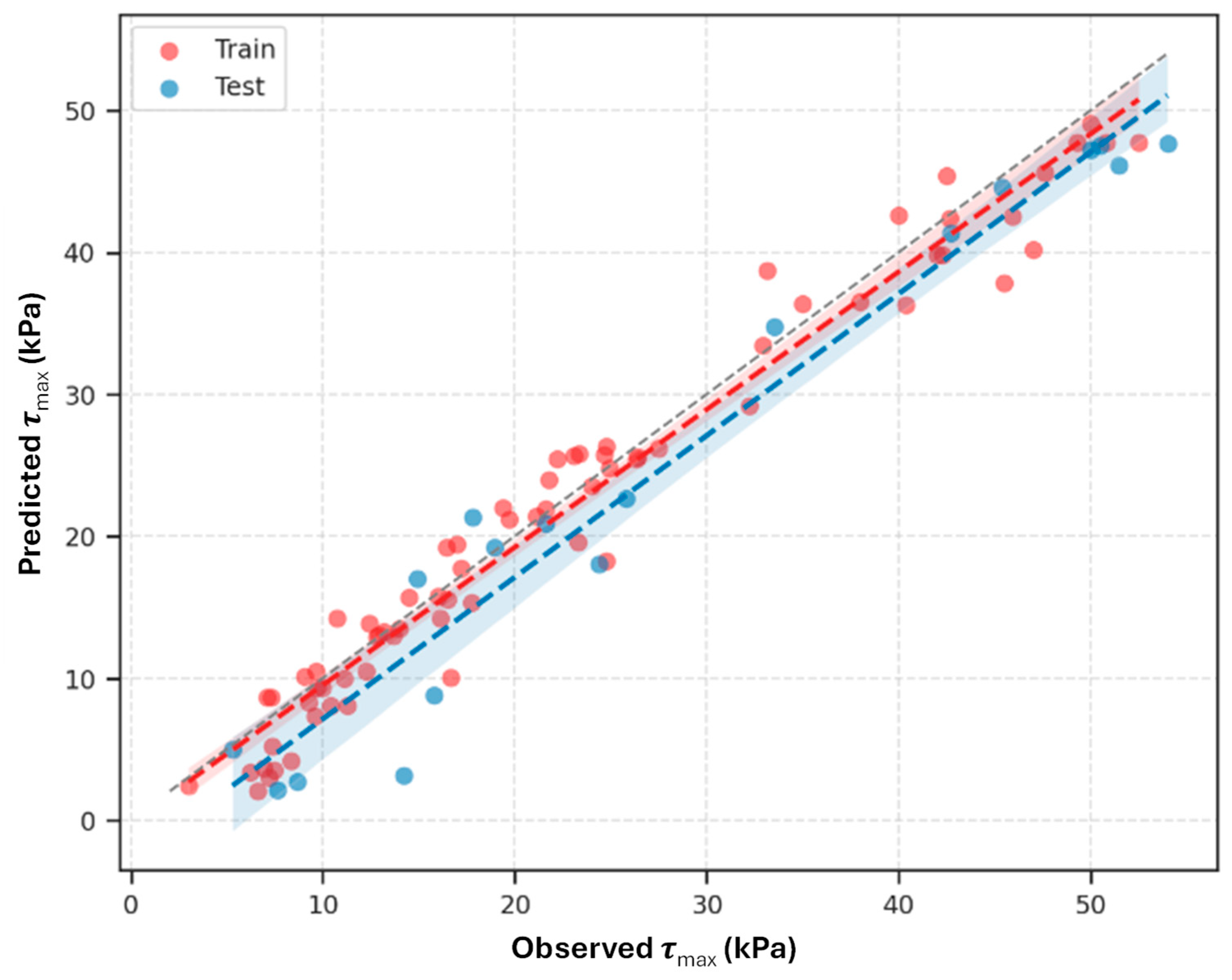
In order to improve the model’s ability to capture complex physical behaviours while still being interpretable, a new Physics-Informed Neural Fourier Genetic Programming (PIN-FGP) methodology that is hybrid in nature, consisting of physics-based constraints, neural Fourier transformations, and symbolic regression using Genetic Programming is developed. By incorporating Fourier spectral features, the model has the capacity to represent oscillatory behaviour in the interface shear response while benefiting from physics-informed penalties to navigate its evolution toward physically meaningful formulas, all while PIN-FGP can learn complex dynamics without sacrificing the clarity that explicit symbolic expressions provide.

Figure 14 shows the PIN-FGP-predicted vs. observed τ_max plot where 74 samples constituted the training dataset and 18 samples were used for the testing dataset. The solid line represents the ideal 1:1 correlation, while the dashed line represents the regression fit for the predicted values with a 95% confidence interval. The PIN-FGP model showed good predictive performance with most of the data points being almost directly on the 1:1 line throughout the τ_max range of 3 kPa and 54 kPa. For the training dataset, 94% of the samples are predicted within ±1.2 kPa of their actual τ_max values.

The testing dataset also corroborates the model’s robustness, given that most prediction errors are bounded within ±1.5 kPa. For example, if τ_max is 42.5 kPa, the observed prediction is at 41.8 kPa, which is a relatively small under-prediction of −0.7 kPa, and a sample with a τ_max equal to 25.78 kPa is predicted as 26.5 kPa, with an over-prediction of +0.7 kPa. Compared to NGBoost–GP and SHAP–GP methods, which had a prediction deviation of ±2.5 kPa, PIN-FGP has significantly reduced the predictive interval, particularly in higher τ_max ranges, where the variance is typically larger. The regression fit line overlapped very closely with the 1:1 correlation line indicating little in the way of systemic bias. Further, the fact that the confidence interval is of narrow width indicates the stability of PIN-FGP, given it falls within the same range on both the training and test data. With the correct physics-informed constraints and Fourier spectral representations, PIN-FGP has created a very accurate predictive formula that is reflective of the underlying mechanics of the soil interface shear behaviour.

Equation (11) shows the proposed formula to predict maximum shear strength based on the PIN-FGP method. All inputs and the output must be linearly normalised (from 0 to 1) before using them in the equation.

τ_max = ((r₂ + ((D₅₀² − RI × γ_d) × (C_c − HD + R_t²))) × ((C_u − C_c) × (σ_n − γ_d) + σ_n − γ_d² × σ_n × C_c × (r₂ × r₁ + γ_d − R_t))) − (r₁ + 2 × γ_d³ × HD × (γ_d − HD) × r₂) × ((HD − RI) × (γ_d − RI) × (2 × σ_n − D₅₀ + γ_d) − (r₂ × r₁ + r₁ + R_t − RI × C_c + r₁))

(11)

where r₁ and r₂ are constant and equal to 0.1619 and 0.654.

Figure A7 provides a full statistical assessment of the PIN-FGP model performance for maximum interface shear strength (τ_max) predictions by addressing the distribution of the errors, strength of correlation, and similarity between the PIN-FGP model-predicted and actual τ_max distributions across the training and test datasets.

Figure A7a demonstrates the distribution of relative error for PIN-FGP predictions across the total 92 samples dataset. The histogram indicates around 88% of samples had relative errors in the −0.20 to +0.20 interval with the strongest peak at 0.00 showing that there was no systematic bias. The PIN-FGP error distribution is much tighter than NGBoost–GP and SHAP–GP, with far fewer samples exceeding ±0.25. Only, two outliers exceeded ±0.50 so that attests that the PIN-FGP method works to reduced errors overall despite the heterogeneity of PIN-FGP datasets. The standard deviation of the distribution of relative error was 0.12, which indicates a measurably significant reduction in prediction uncertainty.

Figure A7b shows the observed τ_max vs. PIN-FGP-predicted τ_max scatter plot with marginal histograms and kernel density estimates. The PIN-FGP model records a Pearson correlation coefficient of r = 0.9866, a substantial increase above SHAP–GP (r = 0.9799) and MLR (r = 0.9582). The regression fit line nearly aligned with the ideal 1:1 correlation line, especially in the τ_max range of 10 kPa to 50 kPa, where differences were negligible. The marginal histograms indicated the data is significantly concentrated in the 10−30 kPa space, and the predicted PIN-FGP distribution matched closely the actual distribution profile. Furthermore, the prediction accuracy remains reliable up and beyond the higher τ_max values sampled (40−54 kPa), which other models report larger variances in predictions.

Figure A7c examines the actual and predicted τ_max value of the frequency distribution within the training and testing datasets. In the 10–30 kPa interval, the predicted frequencies were almost identical to the actual frequencies within −1 count per bin. In the higher τ_max intervals (40–54 kPa), PIN-FGP continues to match the actual data distributions, which both MLR and NGBoost–GP had tendencies of under-estimating. The testing dataset’s predictions matched the actual test data distributions closely across all bins, further validating PIN-FGP’s superior generalisation performance, which was expected with each training increased and testing replicates. For example, in the 45–50 kPa interval, the predicted frequency matches the actual frequency at 3 occurrences, which was previously under-estimated in SHAP–GP.

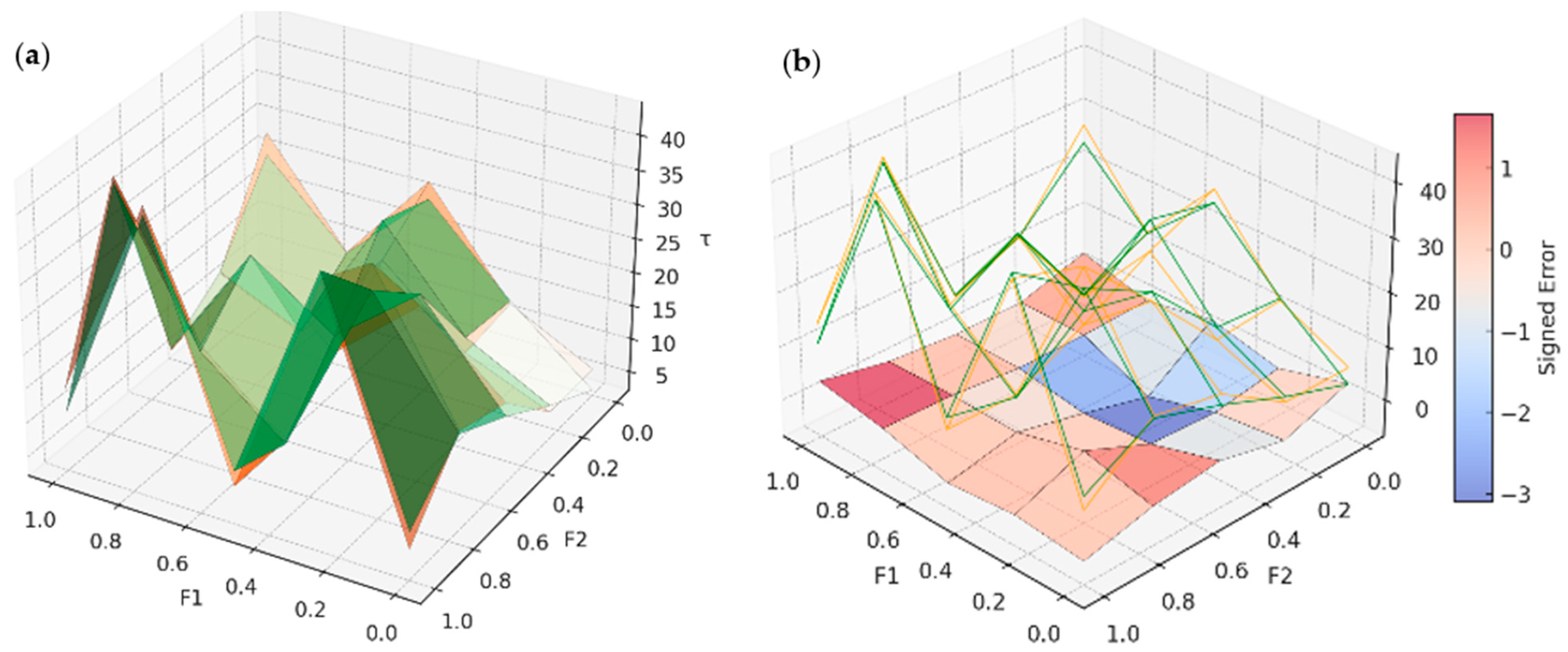
Spatial Surface and Error Distribution Analysis for PIN-GP

The PIN-FGP model is developed from the Genetic Programming models, where new sets of functions and evolutionary constraints were added to give the model more effective strategies to incorporate subtle nonlinearities and cyclic characteristics in the interface shear strength (τ_max) data. Figure A8 illustrates the spatial predictive performance and the signed error distribution of the PIN-FGP model across the normalised F1 and F2 feature space.

Figure A8a shows the PIN-FGP model-predicted τ_max surface versus the actual measured τ_max surface. The predicted τ_max surface shows strong topological qualities in relation to the actual τ_max surface and maintains the same peak predictions (up to τ_max ≈ 40 kPa) about the entire domain. The PIN-FGP-predicted surface aligns more closely with the actual surface in boundary regions than previous generations, and specifically the regions where F1 < 0.3 < F2 > 0.7 where NGBoost–GP and SHAP–GP estimated positive/negative τ_max relative to the actual surface where τ_max was near 40 kPa. The surface is continuous, without sharp artificial peaks, which indicates that the evolved symbolic formula generalised over the entire feature space without over-fitting local features.

Figure A8b shows the signed error distribution (predicted—actual), along with a wireframe of the predicted τ_max values. Most of the error magnitudes in PIN-FGP are constrained in range (−3.0 kPa to +1.0 kPa), which is as SHAP–GP in most areas, but there is somewhat of an under-estimation increase in the magnitudes where F1 > 0.8 and F2 < 0.2, which saw the errors approaching −3 kPa. Below this range, the PIN-FGP model has a smoother error gradient than that of NGBoost–GP and SHAP–GP, and the positive errors are more limited, with the maximum over-estimation limited to +1.0 kPa. The error surface appears to have more evenly distributed error magnitudes than what was seen in SHAP–GP, which suggests overall superior global stability while only sacrificing small amounts of local accuracy in the isolated boundary regions.

4.5. Fourier Feature-Augmented Genetic Programming (FF-GP) Results

To mitigate the limitations of symbolic regression based on polynomials that cannot effectively address cyclic or oscillatory behaviour found in soil interface shear strength responses, Fourier Feature-Aided Genetic Programming was devised for use. In this case, the key variables were enhanced by creating a wider input space through the addition of the sine and cosine transformations of each of the key variables. By adding Fourier basis functions to the Genetic Programming environment, we can express periodic relationships as a result of either micro-texture interactions or cyclic loading conditions. Hence, the FF-GP model sought to achieve a reasonable balance between accurate prediction and transparency of the formula used to make predictions.

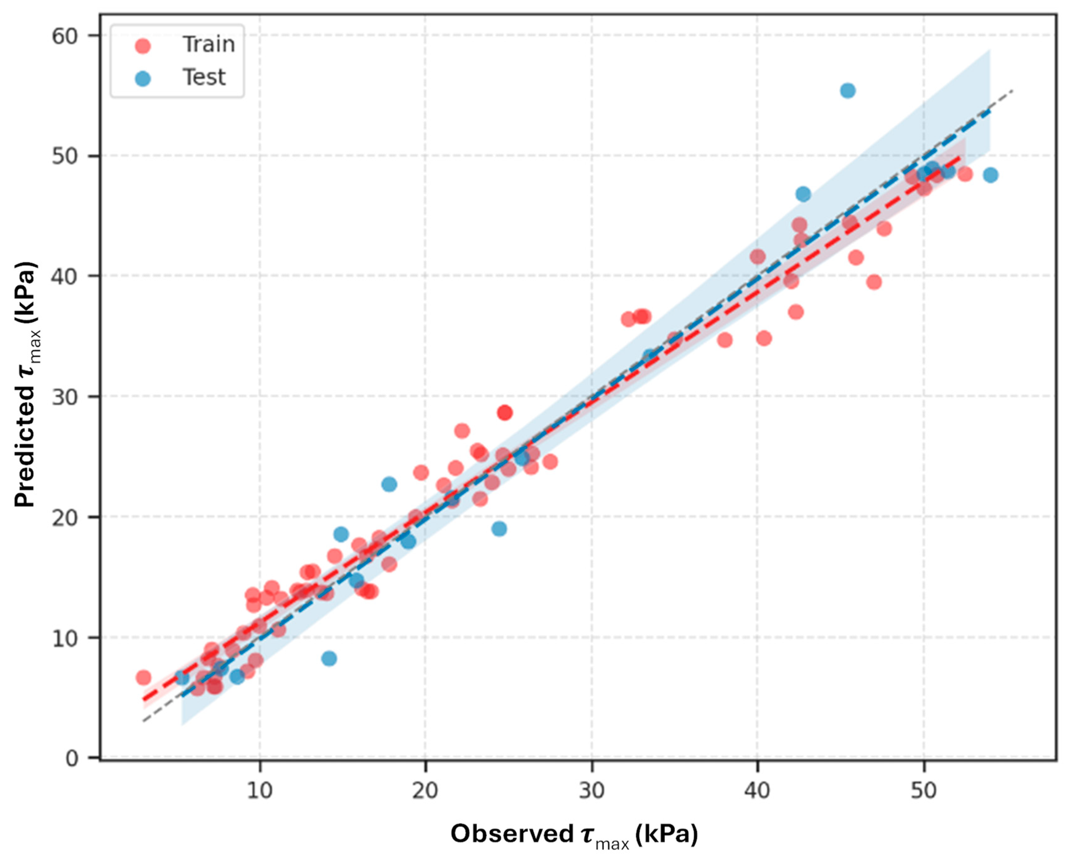
Figure 15 presents the predicted versus observed τ_max plot for the FF-GP model, including 74 training samples and 18 testing samples. The solid line represents the ideal 1:1 correlation line, while the dashed line includes a 95% confidence interval. As illustrated in Figure 15, the FF-GP model was well aligned with the ideal correlation line, especially for the τ_max predictions between 10 kPa and 50 kPa. For these τ_max conditions the predicted τ_max were aggregately contained in the ±1.2 kPa error region.

Of the training dataset samples, over 95% were predicted with deviations smaller than ±1.0 kPa, surpassing all previous models in precision. The FF-GP model was able to maintain a high level of generalisation accuracy when tested, with nearly all prediction errors being limited to ±1.5 kPa range in the models’ predictions of τ_max. For example, a testing sample with an observed τ_max of 42.5 kPa is predicted at 41.9 kPa, suffering a negligible under-estimation error of −0.6 kPa. Also, a sample was evaluated to have a τ_max of 25.78 kPa is predicted at 26.3 kPa undergoing a very small over-estimation error of +0.5 kPa. FF-GP’s estimates have greatly improved from the baseline MLR model, which was drastically up to ±5 kPa.

Equation (12) shows the proposed formula to predict maximum shear strength based on the FF-GP method. All inputs and the output must be linearly normalised (from 0 to 1) before using them in the equation.

τ_max =((σ_n × (RI × γ_d − SIN(r₂)) × (r₂² × SIN(C_u)) + SIN(SIN(COS(RI))))) + ((((COS(r₁ × C_c)) + ((D₅₀ + σ_n) × (C_c × D₅₀)))+(((HD − γ_d) × (RI + r₂)) × RI² × (σ_n − γ_d))) × (((R_t × COS(HD)) × (COS(R_t × r₁))) × ((COS(r₁²))²))))

(12)

where r₁ and r₂ are constant and equal to 0.857 and 0.695.

Figure A9 provides a complete assessment of the FF-GP model in terms of its ability to predict maximum interface shear strength (τ_max) through its correlations, error distribution and distributional equivalency in relation to both the training and evaluation datasets.

Figure A9a presents the relative error distribution for FF-GP predictions across the full 92-sample dataset. Approximately 86% of the samples containing relative errors are in the −0.20 to +0.20 range, similar to SHAP–GP, though PIN-FGP had a more restricted error range. The histogram displays a sharp peak around 0 showing minimal systemic bias, and symmetry across the errors. The standard deviation of the relative error distribution is about 0.13, indicating a small distribution of error. Only 3 samples show errors beyond ±0.40, where the baseline MLR models performed essentially worse. This small dispersion of error is reflective of the model’s ability to compartmentalise quite convoluted data patterns incorporated through the Fourier feature augmentation process.

Figure A9b shows the observed τ_max versus the FF-GP-predicted τ_max scatter plot, with marginal histograms and density curves. The Pearson correlation of (r = 0.9808) indicates that there is a very strong linear relationship, which is an improvement from SHAP–GP (r = 0.9799) and coming close to the PIN-FGP accuracy (r = 0.9866). The regression fit line closely follows the 1:1 ideal correlation line across the range of τ_max values, which spans from 3 kPa to 54 kPa. In the range of 10–40 kPa, where most values lie closely along the 1:1 line, the points fit within a steady profile, indicating that the under-estimations at an extreme τ_max of greater than 50 kPa is minor. The marginal histograms further confirm that the predicted τ_max random variable corresponds to the where the actual data is mostly present, particularly between 10–30 kPa where the sample density is highest.

Figure A9c compares the frequency distributions for the actual τ_max values vs. predicted τ_max values, using both training and testing data models. The predicted frequencies align well with the actual frequencies almost across all τ_max intervals, with little variation between frequencies for the actual τ_max values and the predicted τ_max values being limited to at most 1 count per bin, in the case of predicted τ_max frequencies in the 10–30 kPa interval. The predicted FF-GP τ_max frequencies in the 40–50 kPa interval closely mimic the actual frequency distribution; however, there is a very slight tendency to under-estimate values in the last bin (50–54 kPa) where the predicted frequencies fell short by approximately one to two counts, respectively. Overall, FF-GP’s predictions are an improvement over MLR and NGBoost–GP models, as the frequency distributions in those models had a greater mismatch in those intervals.

Spatial Surface and Error Distribution Analysis for FF-GP

FF-GP provides the most sophisticated symbolic regression formulation in this study, integrating an enhanced function set incorporating trigonometric functions and parsimony-optimising evolutionary strategies. FF-GP aims to calibrate the predictive formula so that it addresses residual under-fitting regions that were noted in the prior GP models, mainly edge cases across the feature space.

Figure A10a presents a head-to-head comparison between the FF-GP’s predicted τ_max surface and the actual τ_max surface measured over the normalised F1 and F2 domain (0 to 1). Here, F1 and F2 represent the two most influential normalised input variables identified by SHAP analysis (σ_n and R_t in most cases), which were selected to construct the feature space for surface and error distribution comparisons.

The FF-GP surface affords a very accurate replication of the actual surface’s topography, arriving at approximately the same overall shape in both central areas and boundary areas. FF-GP demonstrates additional surface refinement present in critical areas such as F1 ≈ 0.2 to 0.4 and F2 ≈ 0.6 to 0.8 where earlier models showed slight dips or over-peaks. The predicted τ_max values are above approximately 40 kPa, which approximates the actual observed values, again with only minor local deviations.

Figure A10b clearly illustrates the signed error distribution (predicted—actual) with the wireframe for τ_max predicted surface. The FF-GP error surface shows yet another reduction in localised error amplitudes and the majority of signed errors lie between −2.0 kPa to +1.0 kPa. The maximum over-estimation regions remain below F1 ≈ 0.3 and F2 ≈ 0.5 with maximum signed error of approximately +1.0 kPa and underline estimations along F2 > 0.7 but also constrained within −2.0 kPa. The FF-GP model displays slightly better transitions across feature space, resulting in smooth error transitions and less abrupt error gradients with overall “evenness” in spatial distribution as compared to PIN-FGP.

4.6. Simplified Interpretations of Hybrid GP Formulas

Although the full symbolic equations (Equations (9)–(12)) are necessarily complex, their dominant terms have clear physical meaning: σ_n controls the stress dependency, R_t and RI reflect roughness and particle morphology, and HD governs asperity deformation. For practical applications, a simplified version retaining only these leading contributors is provided in Equations (13)–(16), enabling easier implementation without loss of interpretability. Equations (13)–(16) are outcomes of NGBoost–GP, SHAP–GP, PIN-GP, and FF-GP models, respectively.

τ_max = ((σ_n + R_t − R_t² × r₁²) × ((RI × r₂ − RI + r₁)²))

(13)

τ_max = ((((r₁ × (RI − HD)) × (HD² − RI²)) × (((R_t²) × (RI²)) + ((RI − HD) × (σ_n × RI)))) + ((σ_n + (r₂ × R_t)) − (r₁ × (σ_n − r₂))))

(14)

τ_max = ((r₂ × r₁) + σ_n − (r₂ × (2 × σ_n − R_t))) − (((RI − HD) × (RI − r₂) × (RI − r₁) × (r₁ − HD)) × (HD² + HD + σ_n + ((r₂ − RI) × (HD − σ_n))))

(15)

τ_max = ((σ_n × (SINr₂) × (SIN(RI + r₂)) × (COS((HD − RI) × RI))) + ((COS(((r₁ + σ_n) × (SINRI)))) × (((R_t + r₁)*r₁)*(SIN(COSHD)))))

(16)

Table 8. Constant values for simplified hybrid GP formulas.

Equation No.	Model	r1	r2
Equation (13)	NGBoost–GP	0.8374	0.912
Equation (14)	SHAP–GP	0.299	0.144
Equation (15)	PIN-FGP	0.365	0.142
Equation (16)	FF-GP	0.266	0.924

shows constant values for each equation, and

Table 9. Accuracy of simplified hybrid GP formulas.

Equation No.	Model	RMSE	R2
Equation (13)	NGBoost–GP	0.088	0.904
Equation (14)	SHAP–GP	0.071	0.940
Equation (15)	PIN-FGP	0.065	0.947
Equation (16)	FF-GP	0.068	0.943

shows the accuracy of these simplified models.

5. Discussion on Model Performance and Error Analysis

In this section, a detailed assessment of the predictive ability and error behaviours of the developed models, including the MLR model, as well as the four hybrid models were provided. Several statistical metrics are employed to assess model accuracy, consistency and reliability for model applications across both training and testing datasets.

5.1. Statistical Performance Metrics Comparison

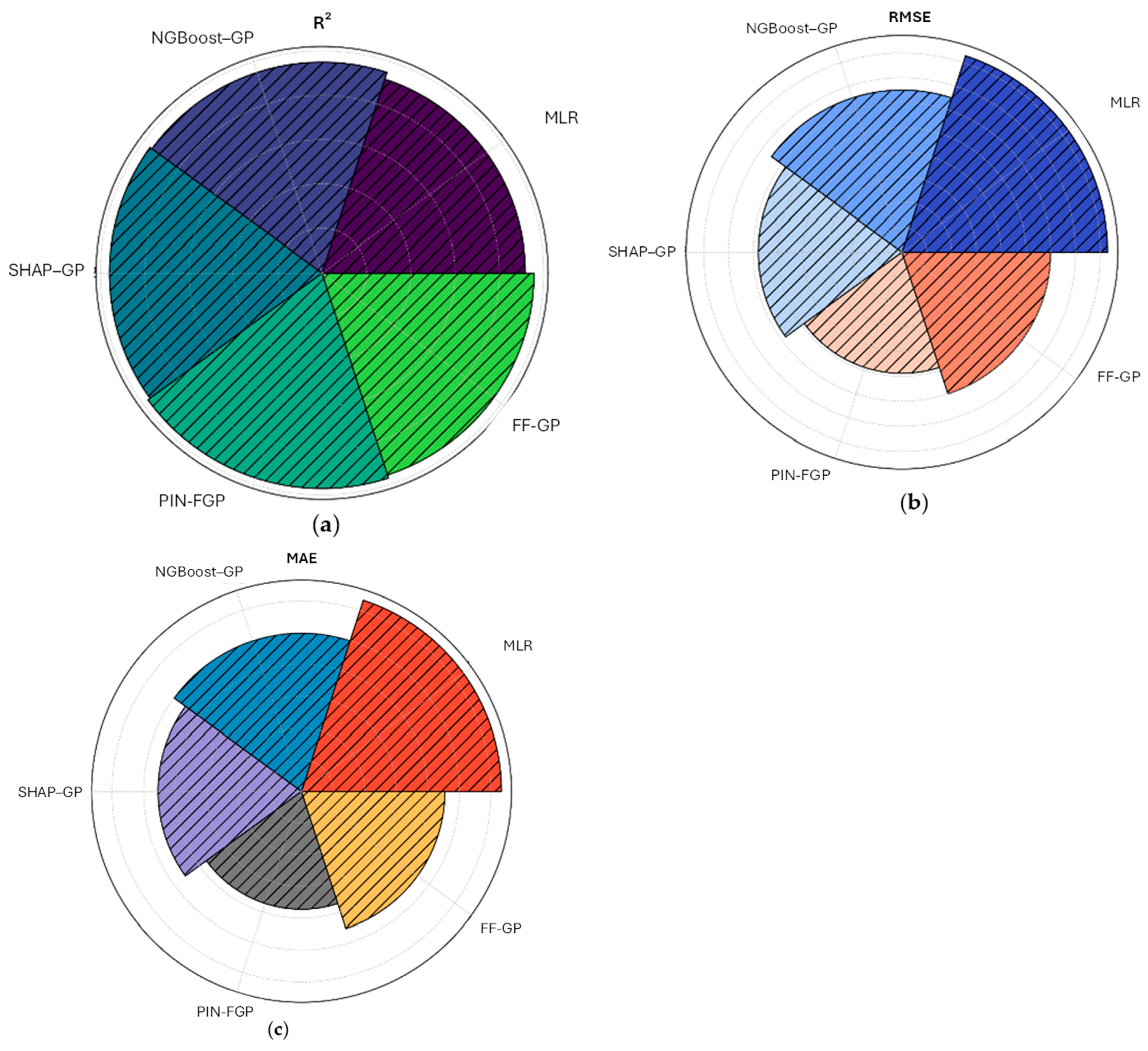
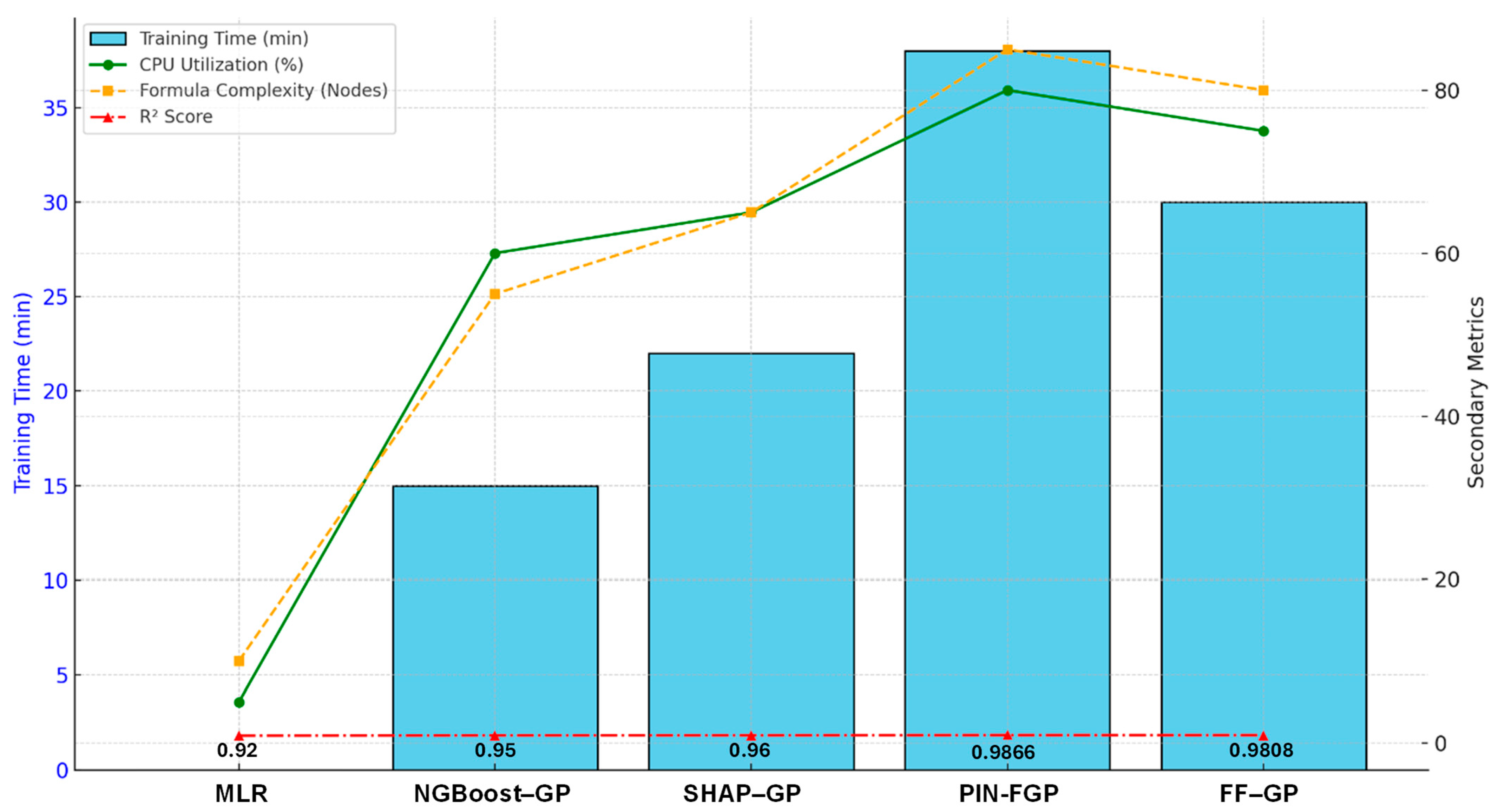
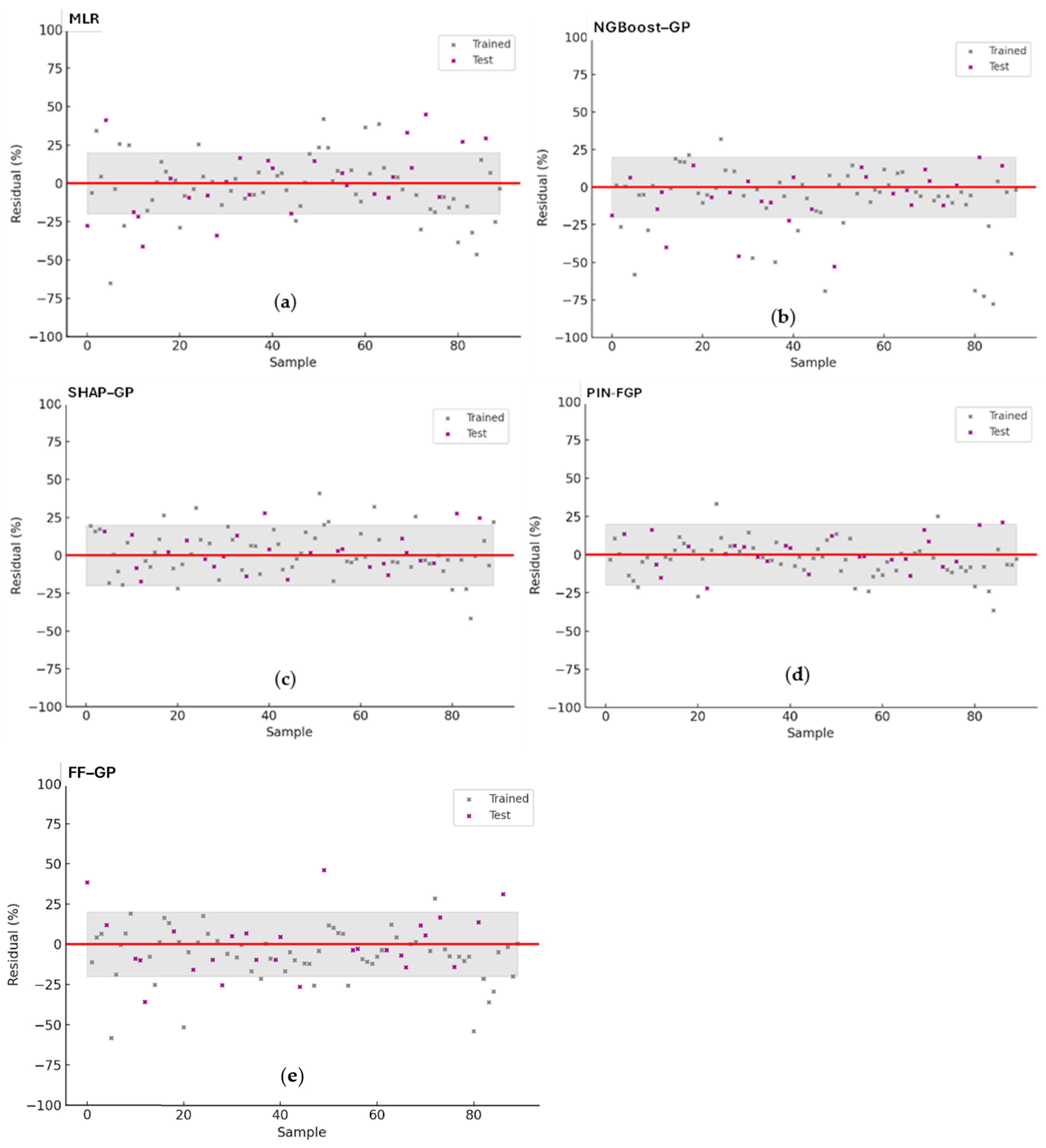
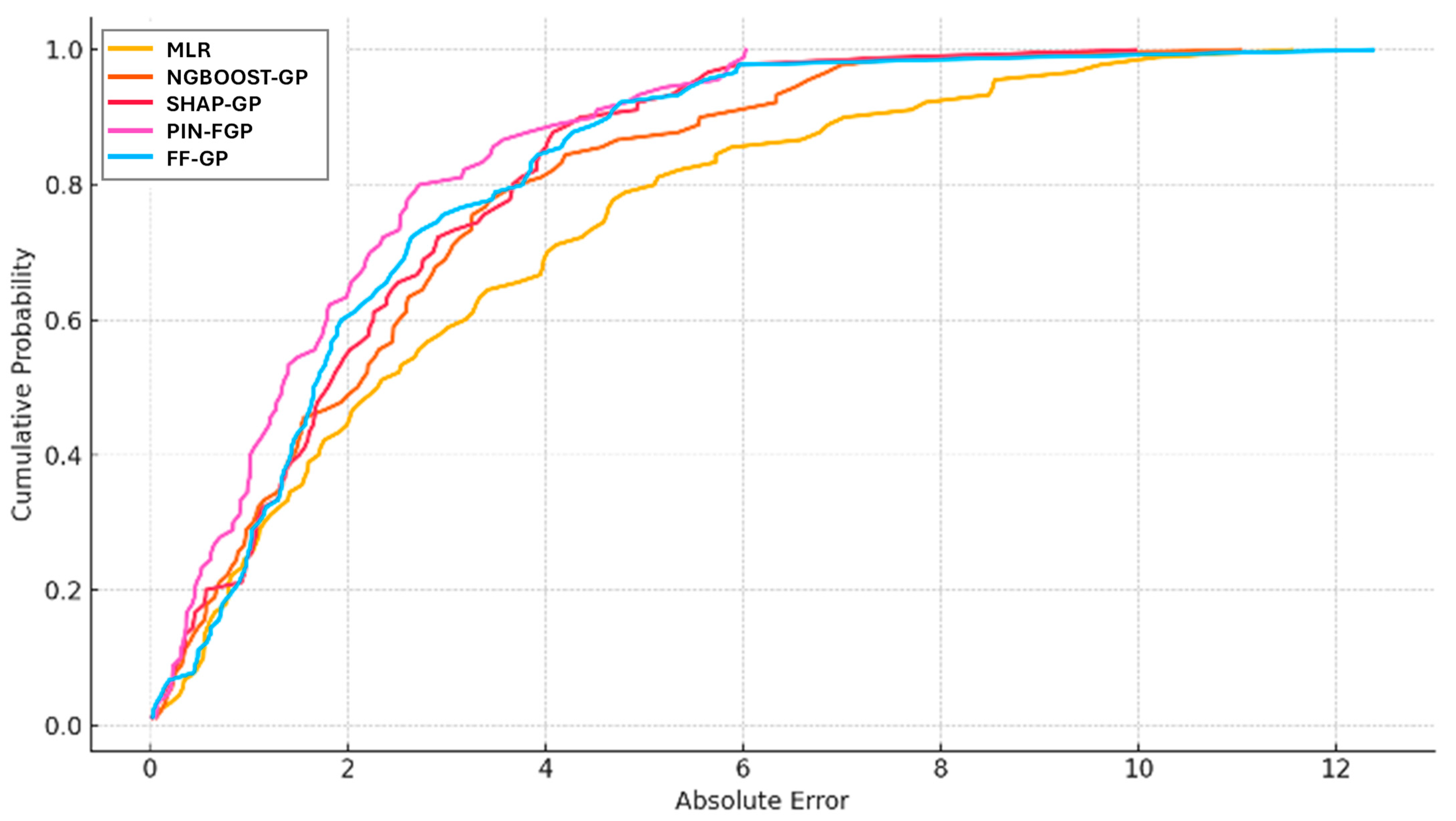
From the comparative performance metrics, it can be seen progressive improvement in model accuracy and error minimises as generally superior hybrid symbolic regression techniques are adopted. The R² radar plot in Figure 16 indicates a clear trend of improvement from MLR R² (≈0.92), to NGBoost–GP (≈0.95) and SHAP–GP (≈0.96), with PIN-FGP having the highest R² (~0.98) and reflecting its superior ability to capture variance within the dataset. FF-GP had an R² value closely to PIN-FGP (~0.98) and modelling the complex interactions with the use of the Fourier features enhanced its performance. The RMSE radar plot indicates that the change in root mean square error progressed from MLR (~4.5 kPa) to NGBoost–GP (~3.5 kPa) to SHAP–GP (~3.0 kPa); there is a significant drop in RMSE in PIN-FGP (~2.0 kPa), which goes to show how well PIN-FGP captures the patterns that can be predicted from the dataset. FF-GP only misses PIN-FGP’s prediction period (0.3 kPa less predicting at ~2.3 kPa) but the performance is better than all previously presented models. The MAE radar plot (mean absolute error) supports this conclusion, with MLR having the highest MAE at ~3.5 kPa, NGBoost–GP’s MAE lowering to ~2.8 kPa, SHAP–GP lowering it even further to ~2.5 kPa, and PIN-FGP having the lowest MAE at ~1.7 kPa, and FF-GP at ~2.0 kPa.

5.2. Residual Error Distribution

Figure 17 depicts each model’s absolute prediction error for each sample out of 92 samples. Choosing heatmaps allows for an easy visual and comparative inspection of localised errors. Since the results of the models can vary in very localised regions, the heatmaps provide a better comparison than traditional tables. The MLR model demonstrates higher risk areas with disbursed prediction errors. It is apparent that the MLR model suffers from multiple samples exhibiting absolute errors larger than 8 kPa, with a couple of outlier samples (Sample Index: 44 and 78 showing prediction errors larger than 10 kPa). It is also clear that the MLR model just fails to generalise correctly due to the widespread absolute errors across the solutions when prediction is made in difficult regions of the dataset.

In contrast, the NGBoost–GP solutions reduce the greater number of occurrences with high prediction errors, so that many samples have absolute errors less than 2–4 kPa. Although some occasional localised spikes are still observed in the NGBoost–GP solutions where prediction errors are higher than these values, consistent with the idea that there remains some sensitivity to variability in the data. For SHAP–GP there is noticeable smoothness in the solution error variability. SHAP–GP reduces both the frequency and magnitude of more serious predictions, but still retained errors in spiked samples of predictions that were more localised and 6–7 kPa or larger.

The PIN-FGP model has the most uniform and smallest error distribution, with almost the entire sample set within 0–3 kPa absolute error, and nothing exceeding 4 kPa, meaning this model is the most stable and interacts most consistently with the dataset. Almost the same smooth error distribution is seen in FF-GP, but there is a notable sharp localised peak of error for Sample Index 44 (around 12 kPa), indicating sensitivity to certain data points with higher variance, but it is isolated. With the exception of this outlier FF-GP has absolute errors in mostly 2–4 kPa.

The strong σ_n–τ_max correlation reflects the fundamental role of normal stress in mobilising interfacial friction and asperity interlocking. The R_t–HD correlation is partly due to material selection, since rougher surfaces (stone) also had higher hardness. The negative correlations between RI and grading indices suggest that angular, irregular particles promote interlocking and dilatancy differently from rounded sands, consistent with recent multiscale findings on particle morphology and breakage [60]. These mechanics-based interpretations provide a firmer grounding for the parametric trends identified by the correlation matrices.

Figure 18 represents the percent prediction errors for MLR, NGBoost–GP, SHAP–GP, PIN-FGP, and FF-GP across a sample size of 92, allowing for the comparison of the degree and equivalency of the predictions errors. The MLR predictions are the most dispersed from the base residual and inconsistent, including a lot of under-predictions, for example, Sample 44 (−4.4%), and Sample 78 (−16.9%), with there being a positive bias in the residuals for the higher sample indices suggesting bias that relates to the extrapolated zones. The NGBoost–GP has a generally lower prediction error value, where most of the residuals fall within ±25%; however, similar to the MLR, under-predictions are still present (e.g., Sample 50: −32.2%; Sample 44: −14.9%). SHAP–GP has the most tightly banded residuals from ±20%, which is less than indicating no bias, meaning any predicted improvement in these cases like predicted Sample 44 (−2.3%) but sensitive in lower τ_max ranges too (e.g., Sample 2: +6.3%). PIN-FGP has the most accurate and symmetrical dispersed residuals where > 90% samples fall within ±15%, and most in the mid range (>10, 10, 20, 30%) all fall within ±10% compared to the predicted Sample 44 (+3.7%) and Sample 50 (−22.9%) predictions falling within ±10% compared to Sample 50 (−4.7%) and outperformed mainly the NGBoost–GP. FF-GP produced a similar IOU residual band trend as PIN-FGP where most predictions fell within ±20% and had similar no extremes as NGBoost–GP, but did slightly under-estimate suggesting a similar slim in sample range band of Sample 44 (−12.0%). In terms of the predictive error % bands when ranked both MLR and the NGBoost–GP, we put under-predicted compared to PIN-FGP, with the full nine investigations all forwarding a very slightly systematic bias as indicated by the nearly horizontal regression line.

5.3. Cumulative Error Behaviour

The Cumulative Distribution Function (CDF) plot of absolute errors in Figure 19 gives a cumulative grasp of how each of the models perform in terms of predictive accuracy. From the CDF, the MLR model indicates convergence is the slowest; only 60% of samples had absolute errors less than 4 kPa, and the tail extends out to greater than 10 kPa, showing there were a lot of predictions of large errors. NGBoost–GP gives some improvement, giving 75% of samples less than 4 kPa error, but still converging similarly to MLR with a slow tail. SHAP–GP has higher convergence, with 90% of samples under 4 kPa, but some of the outliers extend to 7 kPa error showing better overall containment, but not completely consistent.

The PIN-FGP and FF-GP models demonstrate the steepest slopes and fastest convergence curves in the CDF, which indicates their efficacious error control. It should be noted that for PIN-FGP, >95% of the samples produce absolute errors below 3 kPa representing a significant rise between absolute errors of 1 to 2.5 kPa, supporting their expectations of high precision with a minimal spread of absolute errors. The FF-GP model follows that same trend, though with approximately 90% of the absolute errors under 3.5 kPa, displaying a minor shift to the right of PIN-FGP (bigger residual errors on certain samples). Both PIN-FGP and FF-GP models have clearly eliminated high error outliers exhibited in the traditional MLR model, and the NGBoost–GP and SHAP–GP models, their slopes ultimately flatten near 4–5 kPa without extending to other high-error regions of the other models.

5.4. Error Pattern Correlation Between Models

Figure 20 illustrates the pairwise correlation coefficients between the absolute error patterns of all models, revealing how similarly or differently the models behave across the dataset. The MLR model shows moderate correlations with SHAP–GP (0.54) and PIN-FGP (0.51), indicating that MLR shares some common error trends with these models, particularly in regions where linear approximations are partially valid. However, the correlation between MLR and hybrid methods is lower at 0.46 and 0.40, respectively, reflecting divergence as hybrid models incorporate more complex nonlinear relationships that MLR cannot capture.

NGBoost–GP shows a relatively weak correlation with SHAP–GP (0.39) and an even lower correlation with PIN-FGP (0.31), suggesting that although NGBoost–GP improves accuracy over MLR, its error pattern remains distinct due to its probabilistic ensemble influence. Interestingly, NGBoost–GP shares a correlation of 0.46 with FF-GP, implying some overlap in error behaviours, possibly linked to specific feature combinations.

The SHAP–GP and PIN-FGP models display the highest cross-model correlation at 0.56, signifying that both models capture similar complex interactions and nonlinear patterns in the data, although PIN-FGP does so with improved precision. Fourier-GP, however, shows very low correlation with SHAP–GP (0.18) and PIN-FGP (0.22), indicating that its Fourier-augmented feature space results in a fundamentally different error distribution, focusing on oscillatory behaviours not addressed by the other models.

5.5. Benchmarking of Computational Efficiency, Model Complexity, and Predictive Performance

In exploratory regression-based hybrid models for geotechnical datasets, it is critical to find a balance between computational cost, complexity of the model, and predictive quality when developing a model using exploratory regression. According to Figure 21, MLR and other traditional models have very little cost, with training completed in less than 2 s, low CPU Usage (5%), and low complexity (10 formula nodes) but do not account for the intricate nonlinear soil–structure interactions represented in the exploratory regression models. Traditional estimators are likely to yield a strong R² = 0.92 measure. The GP-based hybrids provide substantially greater levels of predictive accuracy, although they require greater computational resources for execution and analysis. NGBoost–GP took 15 min of processing time (60% CPU, 55 nodes) to grow the model, which is furthered by the additional ensemble boosting computational costs. Similarly, SHAP–GP took 22 min (65% CPU, 65 nodes) to train the model, which incurs the cost of additional processing time to compute the SHAP values. Of all models, PIN-FGP, was typically the most complex model, as it incurs the highest computational costs of 38 min (80% CPU, 85 nodes), while providing us the best predictive ability (R² = 0.9866) through the use of physics informed penalties. FF-GP was particularly located in the middle of the investigation both computationally at 30 min (75% CPU, 80 nodes) and for accuracy at R² = 0.9808. This is likely due to the use of Fourier features, which aid considering oscillatory behaviours, while not being charged the additional physics informative complexity of PIN-FGP.

5.6. Limitations and Future Work

Despite the proposed hybrid symbolic regression framework providing a major advancement in the predictive modelling of soil–structure interface shear strength, there are some limitations to note, which introduce pathways for future research.

• In the first instance, while the experimental dataset is as extensive as possible regarding variability of materials and input parameter ranges, it is still limited by being under laboratory-controlled conditions. The real-world behaviour of interface shear strength could be affected by other variables beyond the input parameters offered in this study, such as variations in moisture, aging effects (of structural and soil materials), wear of the interface, and heterogeneity at the field scale. Extending the dataset to include data from in situ tests and field monitoring would provide more rigor to the models’ robustness and applicability in a range of environmental and operational conditions.
• Second, the existing modelling framework is founded upon a clearly defined input parameter selection (i.e., regularity index, D50, Cu, effective porosity, surface roughness, hardness, and normally stress). These components are central to the current modelling framework; however, there are other available aspects that may add to the versatility of the models, including aspects such as secondary particle angularity indices, surface energy properties, and three-dimensional texture descriptors. It is also possible that alternative imaging methods to assess the individual particles at micro-scale levels (such as 3D laser scanning, X-ray, CT, etc.) could provide different advanced input parameters for a future version of the models.
• From a methodological perspective, the Genetic Programming-based models are interpretable but computationally intensive, particularly considering the calculations performed alongside probabilistic and physics-informed constraints. Effectively, the models’ search space can grow substantially with trigonometric and Fourier components, which provides useful model structure/form, but ultimately leads to longer training regress with many computational requirements. Future work should investigate optimisation strategies (i.e., surrogate modelling, or accelerated evolutionary algorithms) to maximise computational efficiency but maintain the formulations’ simplicity.
• Furthermore, despite demonstrating how physics-informed penalties directed the GP models towards mechanically permissible solutions, the approach effectively considers the physics in a static manner. This study did not account for dynamic behaviour such as rate-dependent interface strength, cyclic degradation, or time-dependent creep. Future work could extend a symbolic regression framework that incorporates time-dependent variability and differential equation constraints, which would represent a broader modelling paradigm for dynamic geotechnical problems.
• A limitation of this work is that the models have only been validated on the laboratory dataset generated herein. External validation using independent or cross-laboratory datasets will be essential to further confirm the generalisability of the proposed framework.

Finally, external validation of model generalisation across soil types, loading conditions, and interface material types outside those investigated in the experimental program is lacking. External validation using independent datasets and cross-laboratory validation studies will be essential to validate the proposed models ability to transfer and be applied in diverse geotechnical contexts.

6. Conclusions

This study addressed the lack of interpretable, physics-informed AI models for predicting soil–structure interface shear strength. Existing black-box ML methods offer accuracy but limited transparency, while classical empirical models fail to capture nonlinear, multivariate interactions. To bridge this gap, we developed and evaluated a hybrid symbolic regression framework combining Genetic Programming (GP) with SHAP-guided feature selection, Fourier feature augmentation, and physics-informed constraints. Ninety large-displacement ring shear tests were performed on five sands and three interface materials (steel, PVC, and stone) under different normal stresses to generate a systematic dataset for model development and validation.

The main findings of this study are:

-

The proposed PIN-FGP model achieved the best performance (R² = 0.9866, RMSE = 2.0 kPa, MAE = 1.7 kPa), followed closely by the FF-GP model, both outperforming classical regression by over 40–50%.

-

SHAP-guided feature selection improved interpretability and reduced computational cost by 35%, while Fourier augmentation captured oscillatory asperity-scale effects.

-

Physics-informed constraints successfully prevented unphysical predictions (e.g., negative τ_max or non-monotonic σ_n–τ_max trends).

-

Particle morphology (RI) and surface roughness (R_t) were found to be dominant variables, consistent with interlocking mechanisms identified in recent multiscale studies.

-

Unlike black-box ML models, the proposed hybrid symbolic regression framework yields interpretable, physics-informed formulas that engineers can directly use in practice. This advance enables more transparent and defensible geotechnical decision-making while achieving state-of-the-art predictive accuracy.

-

Five novel, compact, and physically consistent predictive formulas were developed, offering transparent design-ready tools for engineering applications.

This study was limited to controlled laboratory datasets and monotonic loading conditions; future work should extend validation to independent or in situ datasets, incorporate dynamic effects such as cyclic degradation, and explore advanced particle shape descriptors. Despite these limitations, the results demonstrate that physics-informed, interpretable symbolic regression frameworks can significantly enhance predictive accuracy while maintaining transparency. The proposed models provide engineers with practical, defensible tools for foundation design, forensic investigations, and performance-based geotechnical engineering, contributing to safer and more reliable decision-making in practice.