Comparative Analysis and Performance Evaluation of SSC, n-SAC, and Creep-SCLAY1S Soil Creep Models in Predicting Soil Settlement

Abstract

The precise prediction of soil settlement under applied loads is of paramount importance in the field of geotechnical engineering. Conventional analytical approaches often lack the capacity to accurately represent the rate-dependent deformations exhibited by soft soils. Creep affects the integrity of geotechnical structures and can lead to loss of serviceability or even system failure. Over time, they deform, the soil structure can be weakened, and consequently, the risk of collapse increases. Despite extensive research, regarding the creep characteristics of soft soils, the prediction of creep deformation remains a substantial challenge. This study explores soil consolidation settlement by employing three different material models: the Soft Soil Creep (SSC) model implemented in PLAXIS 2D, alongside two user-defined elasto-viscoplastic models, specifically Creep-SCLAY1S and the non-associated creep model for Structured Anisotropic Clay (n-SAC). Through the simulation of laboratory experiments and the Lilla Mellösa test embankment situated in Sweden, the investigation evaluates the strengths and weaknesses of these models. The results demonstrate that the predictions produced by the SSC, n-SAC, and Creep-SCLAY1S models are in close correspondence with the field observations, in contrast to the more simplistic elastoplastic model. The n-SAC and Creep-SCLAY1S models adeptly represent the stress–strain response in CRS test simulations; however, they tend to over-predict horizontal deformations in field assessments. Further investigation is advisable to enhance the ease of use and relevance of these sophisticated models.

1. Introduction

The primary cause of slope failures or landslides and foundation failures is the increased influence of the tangential component of the gravitational force on the potential plane of shear or failure. The tangential component acts along the shear plane, especially composed of soft soil materials that exhibit a higher degree of compressibility compared to other common engineering soil materials. Therefore, the most formidable aspect that must be considered when addressing slope stability, landslides, foundations, or the stability of any other geotechnical structures is the rate of ground settlement under applied loads. This issue has remained contentious, although various methodologies have been reported addressing the issue of soft soil settlement. However, the time-dependent strain, often referred to as the creep phenomenon, has not been thoroughly examined, which might have resulted in the inability to attain the required precision in estimating the material settlement.

To predict the soft soil time-dependent settlement more effectively, the finite element method (FEM) is extensively employed, and the Soft Soil (SS) and Soft Soil Creep (SSC) models, available in the commercial version of PLAXIS 2D [1], are frequently used tools for this purpose. In addition to these two models, other models incorporating creep effects, introduced by Grimstad & Degago [2] and Sivasithamparam [3], respectively, are the non-associated creep model for Structured Anisotropic Clay (n-SAC) and Creep-SCLAY1S. However, these two models are relatively unexplored and remain in an improvement phase, necessitating a thorough examination of their robustness to provide a comprehensive assessment of the accuracy of their outcomes. Moreover, it is also crucial to understand the key input parameters and to validate the performance of these models and enhance their applicability in geotechnical designs.

The time-dependent function of the stress–strain relationship, commonly referred to as creep deformation, extends beyond the classical concept of secondary compression [4,5,6]. Through laboratory tests as well as field observations, the influence of time on the compressibility of clays has been well elucidated by Buisman [7] and Taylor [8]. Buisman ascertains that the settlement in clays increases linearly with the logarithm of time under constant effective stress [7]. Secondary compression describes volume reduction following primary consolidation under constant effective stress, but creep encompasses additional plastic deformations, including deviatoric creep strains, viscosity, and time-dependent resistance. These broader mechanisms have been emphasized in a study by Bjerre [9] to distinguish creep from traditional secondary consolidation behavior.

Suklje [10] proposed an initial model of clay behavior as being determined by a distinctive relationship between the effective stress, void ratio, and strain rate, which postulates that the creep occurs continuously during consolidation, implying that consolidation and creep effects are not discrete processes. Suklje’s model further acknowledges that time-dependent strains are affected by layer thickness, hydraulic conductivity, and drainage conditions. Similarly, Bjerrum [11] introduced a unique correlation between the void ratio, overburden pressure, and time, while also delineating the concepts of instant and delayed compression, where instant signifies strains occurring concurrently with the rise in effective stresses, and delayed denotes strains occurring under constant effective stresses.

Likewise, Janbu [12,13,14] presented the concept of time resistance, asserting that it serves as a potent framework for elucidating the stress- and time-dependent behavior of soils subjected to compression, swelling, or recompression. When an applied load is regarded as an action, the resultant strain is viewed as a reaction. In creep, time is perceived as an action, and the corresponding creep strain is its reaction, as depicted by Equation (1).

$$R_t={\displaystyle \frac{dt}{d\epsilon }}$$

(1)

Laboratory tests have shown that the time resistance of clays increases linearly with time, defining the time resistance number, r_s. The relationship between creep strain and time, derived using the time resistance number, is represented by Equation (2) as follows.

$${\dot{\epsilon }}_{creep}={\displaystyle \frac{\partial {\epsilon }_{creep}}{\partial t}}={\displaystyle \frac{1}{R}}={\displaystyle \frac{1}{r_s(t-t_r)}}$$

(2)

By integrating Equation (2) from t₀ to t, the creep strain over this time period can be estimated, as in Equation (3).

$$\Delta {\epsilon }_{creep}={\displaystyle \frac{1}{r_s}}{\int }_{t_0}^t{\displaystyle \frac{1}{(t-t_r)}}.dt={\displaystyle \frac{1}{r_s}}\mathit{ln}{\displaystyle \frac{(t-t_r)}{(t_0-t_r)}}$$

(3)

Also, the time resistance number, r_s, can be calculated using Equation (4).

$$r_s={\displaystyle \frac{\partial \ln t}{\partial {\epsilon }_{creep}}}$$

(4)

At present, numerous soil models have been devised to address the characteristics of soils, particularly those pertaining to soft soil behavior. In this research, the Soft Soil Creep model (available in PLAXIS 2D [1]), along with two additional user-defined creep models developed by Grimstad [15] and Sivasithamparam et al. [16], which integrate creep effects, have been utilized. These soil creep models are briefly introduced in the following subsections.

1.1. Soft Soil Creep Model

The Garlanger model [17] is one of the earliest frameworks used to model time-dependent behavior in soft clays. It introduces a logarithmic relationship between the void ratio and time under constant effective stress, based on secondary compression. This model is empirical and straightforward, assuming that time-dependent settlement occurs linearly with the logarithm of time. In contrast, the ABC model (also known as the Advanced Block Creep model or ABC Delft model), developed by den Haan [18], incorporates a more advanced rheological approach. It accounts for both elastic and plastic strains and models the strain rate as a function of time, stress level, and viscosity. The ABC model uses a time resistance concept that enables it to represent non-linear creep, anisotropy, and stress-path dependency more realistically, especially under varying loading conditions.

The Soft Soil Creep model was formulated to account for the secondary compression in soft soil. The total strain comprises two components: one representing the elastic portion, and the other denoting the inelastic viscoelastic or creep component [7,17,19], with the inelastic portion occurring not only under constant effective stresses but also incorporated into the consolidation phase. Hence, the equation of the total strain (under the one-dimensional condition) can be expressed as follows (Equation (5)).

$$\epsilon =A\ln \left({\displaystyle \frac{{\sigma }^{\prime }}{{\sigma }_0^{\prime }}}\right)+B\ln \left({\displaystyle \frac{{\sigma }_c^{\prime }}{{\sigma }_{c,0}^{\prime }}}\right)+C\ln \left({\displaystyle \frac{{\tau }_c+t^{\prime }}{{\tau }_c}}\right)$$

(5)

where the first component signifies the elastic strains resulting from an increase in effective stress over the specified time period t. The subsequent component accounts for the creep strains during the consolidation phase, characterized by the increase in preconsolidation pressure from the beginning of loading to the end of primary consolidation. The last component represents a pure creep strain under constant effect stress, begun from the end of the consolidation, t’. Currently, this model is extensively used in geotechnical engineering as creep deformation is a primary concern. More details can be found in the PLAXIS 2D Material Models Manual [1,20] and in the works of Vermeer & Neher [21].

1.2. Creep-SCLAY1S Model

The Soft Soil Creep (SSC) model, widely implemented in commercial software such as PLAXIS, extends the modified Cam Clay framework by incorporating time-dependent volumetric plastic strains. Creep is introduced through a viscoplastic formulation where the strain rate depends on the stress level and a creep index, assuming an associated flow rule. While the SSC model is effective for isotropic creep conditions, it does not account for anisotropy or destructuration, which limits its applicability to natural structured soils.

In contrast, the Creep-SCLAY1S model, developed by Karstunen et al. [22] and further advanced by Grimstad et al. [23], introduces anisotropic viscoplastic behavior, incorporating mechanisms such as rotational hardening, destructuration, and evolving anisotropic yield surfaces. A key innovation is the use of a plastic multiplier formulation in conjunction with the creep index (μ*), which regulates the rate of creep strain accumulation. This multiplier is further constrained by a minimum void ratio, preventing unrealistic long-term deformation. These enhancements allow Creep-SCLAY1S to better capture the mechanical response of natural soft clays under long-term loading conditions and stress-path-dependent behavior.

Destructuration refers to the breakdown of the soil’s internal structure, typically caused by loading or prolonged creep. This process leads to a reduction in strength and stiffness over time. Fabric anisotropy and “destructuration” are phenomena frequently observed in natural clay. To integrate these characteristics into the time-dependent behavior while also achieving the enhanced creep behavior of soft clays, a novel anisotropic creep model designated as Creep-SCLAY1S was proposed by Sivasithamparam [3]. In Creep-SCLAY1S, the magnitude of the plastic multiplier in conjunction with the creep index is delineated as follows.

$$\stackrel{·}{\Lambda }={\displaystyle \frac{{\mu }^{\prime }}{\tau }}{\left({\displaystyle \frac{p_{eq}^{\prime }}{p_p^{\prime }}}\right)}^{\beta }\left({\displaystyle \frac{M^2-{\alpha }_{K_0^{NC}}^2}{M^2-{\eta }_{K_0^{NC}}^2}}\right)$$

(6)

where $\tau$ is the reference time; $p_{eq}^{\prime }$ is the equivalent mean stress; $p_p^{\prime }$ is the preconsolidation pressure; M is the slope of the critical state line; and ${\mu }^{\prime }$ is the modified creep index as in SSC. An associated flow rule is presumed, thereby allowing the creep strain rate to be estimated as in Equation (7).

$$\Delta \dot{{\epsilon }_{ij}^c}=\stackrel{·}{\Lambda }{\displaystyle \frac{\partial p_{eq}^{\prime }}{\partial {\sigma }_{ij}^{\prime }}}$$

(7)

Likewise, the increment of plastic strain is determined by using the plastic multiplier of Equation (8). More details can be seen in the works of Sivasithamparam [16,24].

$$\Delta \dot{{\epsilon }_{ij}^c}=\stackrel{·}{\Lambda }\Delta t{\displaystyle \frac{\partial p_{eq}^{\prime }}{\partial {\sigma }_{ij}^{\prime }}}$$

(8)

1.3. Non-Associated Creep Model for Structured Anisotropic Clay (n-SAC)

Previously established various elastoplastic models employed an associated flow rule [25,26]. Nevertheless, laboratory investigations on natural soil indicate that this presumption is insufficient. Recognizing this reality, a new model known as the non-associated creep model for Structured Anisotropic Clay, or n-SAC for short, was introduced by Grimstad & Degago [2]. In contrast to the SSC model, this model employs the time resistance concept to simulate the creep behavior; it utilizes a non-associated flow rule, implements a distinct rotational hardening law for the two surfaces, and adopts a destruction rule [15,23]. By employing time resistance instead of the volumetric viscoplastic strains theory, the rate of the plastic multiplier is articulated by the following equation (Equation (9)), as proposed by Grimstad & Degago [2].

$${\displaystyle \frac{d\lambda }{dt}}={\displaystyle \frac{1}{r_{si}\tau }}{\left({\displaystyle \frac{p^{eq}}{(1+x)p_{mi}^{\prime }}}\right)}^{r_{si}{\xi }_i}{m}_{K_{0}NC}$$

(9)

where ${\xi }_i$ is the intrinsic viscoplastic compressibility coefficient; $r_{si}$ is the intrinsic time resistance number; $p^{eq}$ is the equivalent stress; $p_{mi}^{\prime }$ is the intrinsic reference stress; $\tau$ is the reference time; $x$ is the amount of instable structure; and $m_{K_{0}NC}$ is given by Equation (10).

$$m_{K_{0}NC}={\displaystyle \frac{M_{fC}^2-{\alpha }_{K_{oNC}}^2}{M_{fC}^2-{\mathsf{\eta }}_{K_{oNC}}^2}}$$

(10)

where ${\mathsf{\alpha }}_{K_{oNC}}$ is the rotation (fabric) of the potential surface under $K_0^{NC}$ loading (virgin oedometer loading); ${\eta }_{K_{oNC}}$ is the mobilization in $K_0^{NC}$ loading; and $M_{fC}$ is the critical state line in compression loading. Mobilization under K₀ loading in normally consolidated soils refers to the progressive activation of shear strength as vertical stress increases. As the stress state approaches the yield surface without lateral strain, deviatoric stress develops, mobilizing frictional resistance and initiating plastic deformation, particularly in models incorporating anisotropy and creep. More details can be seen in the works of Grimstad [15,27].

Considering the development of the above three sophisticated constitutive material models that incorporate creep behavior, a systematic comparison of their efficiency at both the element and field levels has some interest. This prompts essential research queries: how the performance of these constitutive models compare at the element level; which variations occur in their performance when applied in boundary value problems, particularly concerning the importance of anisotropy, destructuration, and creep; and finally, to what degree the simulation outcomes correspond with empirical observations, and what conclusions can be inferred from any inconsistencies.

The capabilities of the model at the element level and boundary value level are illustrated, the latter being evidenced through comparisons with real test observations from the Lilla Mellösa test embankment in Sweden. This permits an examination of the influence of evolving anisotropy and creep at the boundary value level via systematic evaluations. Addressing these queries will enhance the comprehension of each model’s advantages and limitations, thereby informing future advancements and applications.

2. Material and Method

2.1. General Description of Lilla Mellösa Test Embankment

Lilla Mellösa is situated in proximity to Upplands Väsby, to the north of Stockholm, Sweden. The test embankment was erected by the Swedish Geotechnical Institute (SGI) in the year 1945, with the primary objective of identifying a suitable location for a new airfield intended to be established outside the Swedish capital, Stockholm. Ultimately, Lilla Mellösa was deemed inappropriate for airport development, leading to the construction of the airfield at Halmsjön, which is presently recognized as Stockholm Arlanda Airport [28].

The conditions that rendered Lilla Mellösa unsuitable for airport purposes proved to be exceptionally favorable for establishing a geotechnical test site, attributable to the subsoil characteristics comprising 10 to 15 m of highly compressible soils. Over an extended duration, the clay has undergone consolidation under the weight of the fill. The data obtained from this test site is distinctive in the context of long-term monitoring and data acquisition, extending back to the mid-1940s [29,30].

2.1.1. Soil Conditions

The top layer is composed of a 0.3 m thickness of organic topsoil. Prior to the construction of the fill, this layer was removed. Beneath this, a dry crust measuring 0.5 m in thickness comprises organic soil. The underlying soft clay layers extend to 14 m in depth, exhibiting variable organic content throughout the profile. Beneath the soft clay, a thin sand stratum is situated above the bedrock, although it holds lesser significance [28]. The clay layer exhibits elevated water content, reaching a maximum of approximately 130% in the upper section, gradually decreasing to 70% at the lower depths. The undrained shear strength, ascertained through vane shear tests, reveals a minimum value of 8 kPa at a depth of 3 m, with an incremental increase of 1.3 kPa/m thereafter. The clay layer presents varved characteristics beyond a depth of 10 m [28].

2.1.2. Test Fill

The construction of the test fill occurred during the months of October and November in 1947. The fill comprises a 2.5 m high layer of gravel, characterized by a density of 1.7 t/m³. The base dimensions of the fill measure 30 m by 30 m, with a slope ratio of 1:1.5. The construction process necessitated a duration of 25 days for completion, and the load has remained unaltered since that time, aside from natural fluctuations. The net load increase imposed on the fill was calculated to be 40.6 kPa. Following a period of 20 years, the fill experienced settlement below the groundwater table, attributed to hydraulic uplift, with an estimated overburden load amounting to approximately 27 kPa [30].

2.1.3. Measured Settlements and Pore Pressures

Field measurements of settlements and pore pressures in Lilla Mellösa have been recorded since 1945. Before the construction of the test fill, multiple piezometers and settlement markers were installed at different depths in the ground.

The preliminary settlement observed during the brief construction duration was quantified at 0.065 m. Following a consolidation period of 21 years, the surface settlements escalated to 1.40 m, while the excess pore pressure remained approximately 30 kPa during that period. In 1979, the cumulative settlements measured had risen to 1.65 m, with the residual pore pressure still exceeding 20 kPa. The most recent measurement data, which is available from 2002, is documented in SGI report 70 [31], indicating an overall settlement of 2 m and an excess pore pressure close to 10 kPa.

2.2. Methodology

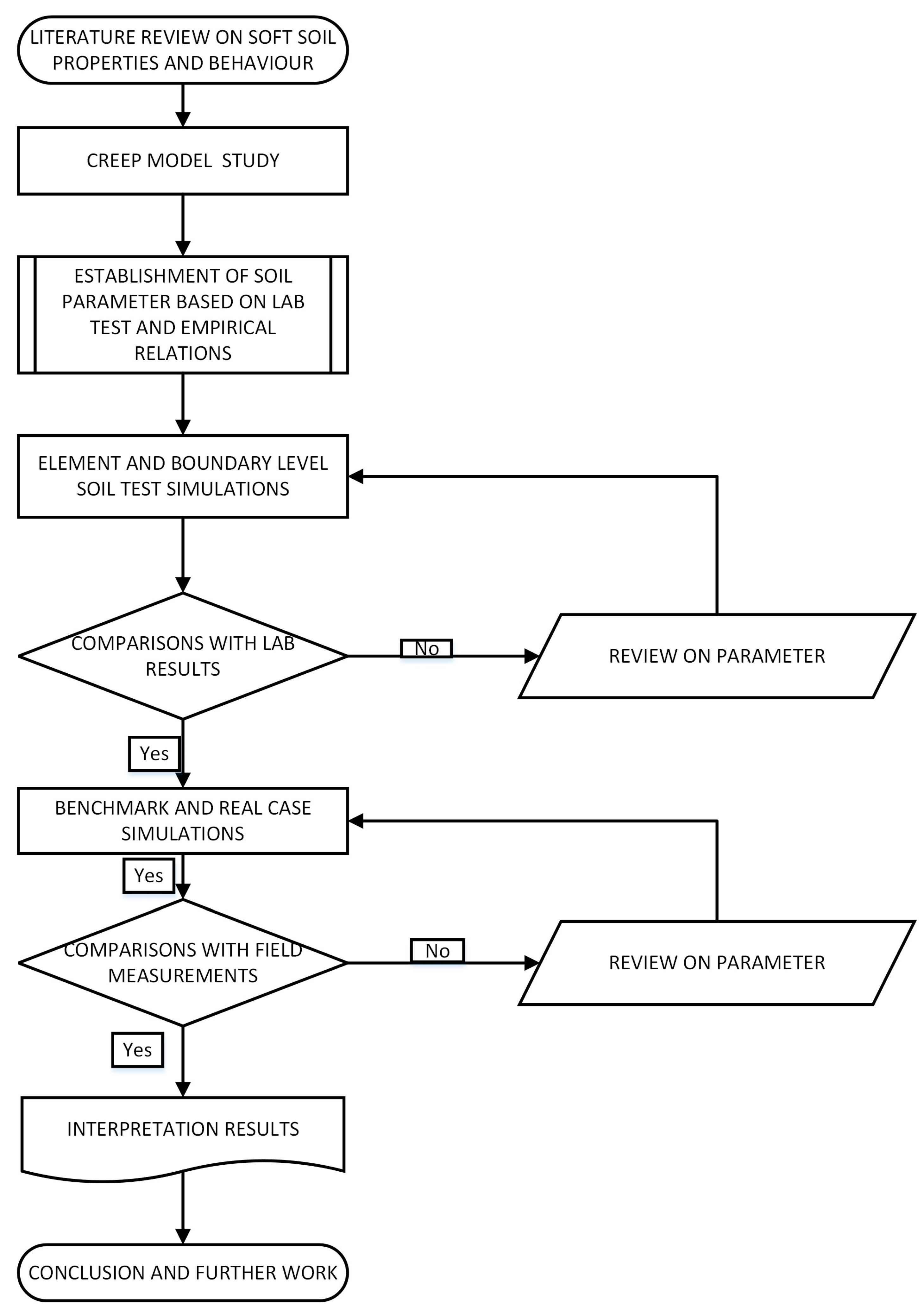
The numerical analysis will utilize the finite element analysis software PLAXIS 2D (ver. 2013.01). It provides precise simulation tools to capture gradual soil movement and strength loss over time, allowing the assessment of potential long-term effects on stability. The chosen material models are designed to accommodate creep deformations. The investigation is structured into several phases, as illustrated in Figure 1. The initial phase entails a comprehensive literature review aimed at gathering pertinent background knowledge regarding the time-dependent settlement of soft soils, considering aspects such as anisotropy, non-linearity, destructuration, and creep. Subsequently, the fundamental characteristics, formulations, and parameters essential for the advanced soil models SSC, Creep-SCLAY1S, and n-SAC were meticulously examined. In the following phase, the methodologies utilized to determine the critical soil parameters essential for these models, alongside standard testing procedures, were assessed. To evaluate the impact of parameters within the model, a comparative analysis among the models was conducted, accompanied by a detailed review of soil test simulations. Constitutive model parameters were derived from laboratory tests and supplemented by interpreted data from SGI reports and approaches as mentioned by Gustafsson and Tian [32] and Karstunen et al. [33]. For SSC, parameters such as λ*, κ*, and OCR were obtained using conventional procedures. For Creep-SCLAY1S and n-SAC, parameters involving creep, anisotropy, and destructuration (e.g., rate of rotation, bonding ratio, and destruction rate) were calibrated using a trial-based optimization process. To clarify parameter determination, we elaborated that parameters for SSC were obtained from SGI lab data and interpreted curves, while for Creep-SCLAY1S and n-SAC, advanced parameters like the rate of rotation and bonding were approximated based on the literature and calibrated using trial-and-error simulation. A detailed description of this determination and sensitivity analysis details are provided in the Supplementary Materials.

Moreover, the contextual background and relevant data from the field case study concerning the Lilla Mellösa test embankment in Sweden were thoroughly scrutinized, and the necessary input soil parameters were determined based on the available field and laboratory data. Ultimately, a comparative evaluation was executed between the computed outcomes obtained from the finite element program PLAXIS 2D and the values recorded in the field. A back-calculation procedure was undertaken to ascertain realistic values for the input parameters in the event of any discrepancies.

2.3. Establishment of Input Parameters

The input parameters for different models are calculated from the information provided in Swedish Geotechnical Institute (SGI) report 29 [28] and report 70 [31], by using the available field investigations and lab results using different approaches as mentioned by Gustafsson and Tian [32] and Karstunen et al. [33]. The established material parameters for SSC are presented in

Table 1. Soil parameters for the SSC model.

Parameters	Identification	Unit	Unit I (0–2.5 m)	Unit II (2.5–7.5 m)	Unit III (7.5–13.8 m)	Unit IV (13.8–14 m Sand)
γ	Unit weight	kN/m3	13	15	16	18
λ*	Modified swelling index	[-]	0.18	0.22	0.29	-
κ*	Modified compression index	[-]	0.006	0.07	0.01	-
μ*	Modified creep index	[-]	0.01	0.009	0.007	-
c	Cohesion	kN/m2	1	1	1	0.05
φ (phi)	Friction angle	°	30	30	30	40
ψ (psi)	Dilatancy angle	°	0	0	0	10
OCR	Initial over-consolidation ratio	[-]	-	1.2	1.3	-
POP	Pre-overburden pressure	[kN/m2]	16	-	-	-
kx/ky	Coefficient of permeability	m/day	6.00 × 10−5	8.60 × 10−5	8.60 × 10−5	6.00 × 10−1
ck	Change in permeability	-	3	3	3	-

, and the properties of the fill materials, topsoil, dry crust, and bottom sand layers are delineated in

Table 2. Soil parameters of fill materials, top soil, dry crust, and bottom sand layers.

Parameters	Identification	Unit	Dry Crust (Linear Elastic)	Fill (Mohr–Coulomb)	Unit IV (13.8–14 m Sand) Hardening Soil
γ	Unit weight	kN/m3	20	17	18
E/E50ref	Young’s modulus	[-]	1.10 × 104	4.00 × 104	2.50 × 104
ν	Poisson’s ratio	[-]	0.3	0.3
c	Cohesion	kN/m2		0.025	0.05
φ	Friction angle	°		37	40
ψ	Dilatancy angle	°		0	10
kx/ky	Coefficient of permeability	m/day	1.18 × 10−4	0.01	6.00 × 10−1

. In a similar manner, the established parameters for Creep-SCLAY1S and n-SAC are presented in

Table 3. Soil parameters for the Creep-SCLAY1S model.

Parameter	Description	Unit	Soil Unit I (0–2.5 m)	Soil Unit II (2.5–7.5 m)	Soil Unit III (7.5–13.8 m)
κ*	Modified swelling index	[-]	0.005	0.0064	0.0085
ν	Poisson’s ratio	[-]	0.15	0.15	0.15
λ*	Modified compression index	[-]	0.18/0.08 *	0.25/0.07 *	0.27/0.07 *
Mc	Critical state constant in compression	[-]	1.2	1.2	1.2
Me	Critical state constant in extension	[-]	0.86	0.86	0.86
ω	Rate of rotation	[-]	30	30	30
ωd	Rate of rotation by deviator strain	[-]	0.76	0.76	0.76
ξ	Rate of destructuration	[-]	0/10 *	0/10 *	0/10 *
ξd	Rate of destructuration by deviator strain	[-]	0/0.1 *	0/0.09 *	0/0.09 *
OCR	Over-consolidation ratio	[-]	0	1.5	1.5
POP	Pre-overburden pressure	[kN/m2]	16	-	-
e0	Initial void ratio	[-]	3.25	2.86	1.9
α0	Initial inclination in p′−q plane	[-]	0.45	0.45	0.45
χ0	Initial amount of bonding	[-]	0/5 *	0/5 *	0/5 *
τ	Reference time	[day]	1	1	1
µ*	Modified creep index	[-]	0.01	0.009	0.007
* indicates a value calculated by considering destructration.

and

Table 4. Soil parameters for the n-SAC model.

Parameter	Description	Unit	Soil Unit I (0–2.5 m)	Soil Unit II (2.5–7.5 m)	Soil Unit III (7.5–13.8 m)
$K_0^{NC}$	Lateral earth pressure ratio in NC region	[-]	0.5	0.5	0.5
ν	Poisson’s ratio	[-]	0.15	0.15	0.15
$t_{max}$	Time to limit for OCR	[day]	1.33 × 105	1.33 × 105	1.33 × 105
$E_{oed}^{ref}$	Reference oedometer modulus	[kN/m2]	930	1100	1250
ω	Rate of destructuration by deviator strain	[-]	0.3	0.3	0.3
$E_{ref}$	Reference modulus	[kN/m2]	42,000	33,000	23,000
φcs	Critical state friction angle	[-]	30	30	30
φp	Peak friction angle	[-]	30	30	30
OCRτ	Over-consolidation ratio	[-]	-	1.2	1.4
POP	Pre-overburden pressure	[kN/m2]	16	-	-
Pref	Reference pressure	[kN/m2]	100	100	100
τ	Reference time	[day]	1	1	1
rs min	Minimum measured time resistance number	[-]	66	70	100
rsi	Intrinsic time resistance	[-]	660	700	1000

, respectively.

The clay layers are segmented into three units to capture the variation of soil properties with depth accurately. The fill material is modeled using the Mohr–Coulomb (MC) model. The topsoil and dry crust are modeled using a linear elastic model, while the deeper sand layers are simulated with the Hardening Soil (HS) model, which is well-suited for capturing non-linear stress–strain behavior and stress dependency in granular soils [34]. The model parameters are established in accordance with the available field investigations and laboratory results, employing various approaches as mentioned by Gustafsson and Tian [32] and Karstunen et al. [33]. Two distinct sets of parameters are applied in the Creep-SCLAY1S model, one incorporating destructuration and the other excluding it.

2.4. Modeling of Constant Rate of Strain (CRS) Lab Tests

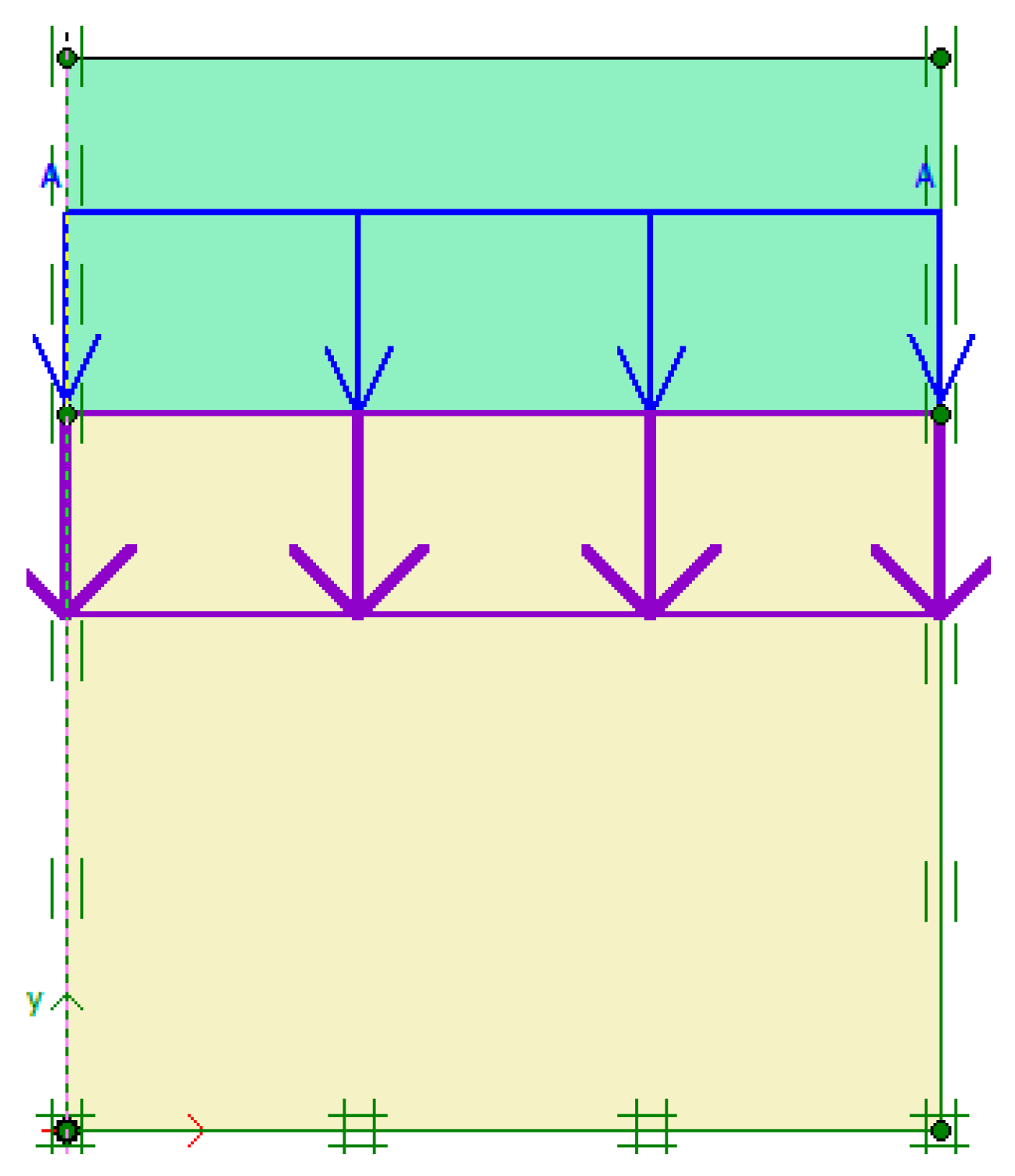
The modeling of the CRS test is performed to verify the accuracy of the parameters previously established for the soft clay layer. The CRS oedometer test is widely employed when determining the parameters requisite for calculating settlement [35]. To back-calculate a CRS oedometer test in PLAXIS2D (ver. 2013.01), an axis-symmetric geometrical model is created, measuring 25 mm in the x-axis and 20 mm in the y-axis, to simulate a standard CRS test specimen that is 20 mm in height and 50 mm in diameter (Figure 2). The boundary conditions are set to the standard constraints available in PLAXIS.

The hydraulic conditions are configured with one-sided drainage at the upper portion, while the remaining three sides are subjected to a sealed boundary condition. The unit weight of the soil sample is designated as zero to establish constant initial stresses. Figure 2 exemplifies the geometrical model as delineated in PLAXIS. The simulation of the test for soil depths of 5 m and 9 m is executed by adhering to the outlined procedure and is subsequently compared with the laboratory test results.

A thin elastic dummy soil layer is applied at the top of the 2 cm test specimen during the initial K₀ calculation phase, which corresponds to the effective overburden stress. This procedure is undertaken to generate the initial in situ stress within the sample. During the first calculation phase, the dummy soil is unloaded to mimic the transition of the sample from the field to the laboratory, while a minor isotropic stress is applied to the sample to account for the remaining effective stress after the allowed swelling following the unloading. This operation is typically conducted under drained conditions and in a relatively expedited manner. Subsequently, the displacement is reset to zero, and the CRS test simulation is started in consolidation analysis mode by applying a predetermined displacement over a defined time interval, which aligns with the strain rate used in the laboratory tests (0.6% per hour in this case).

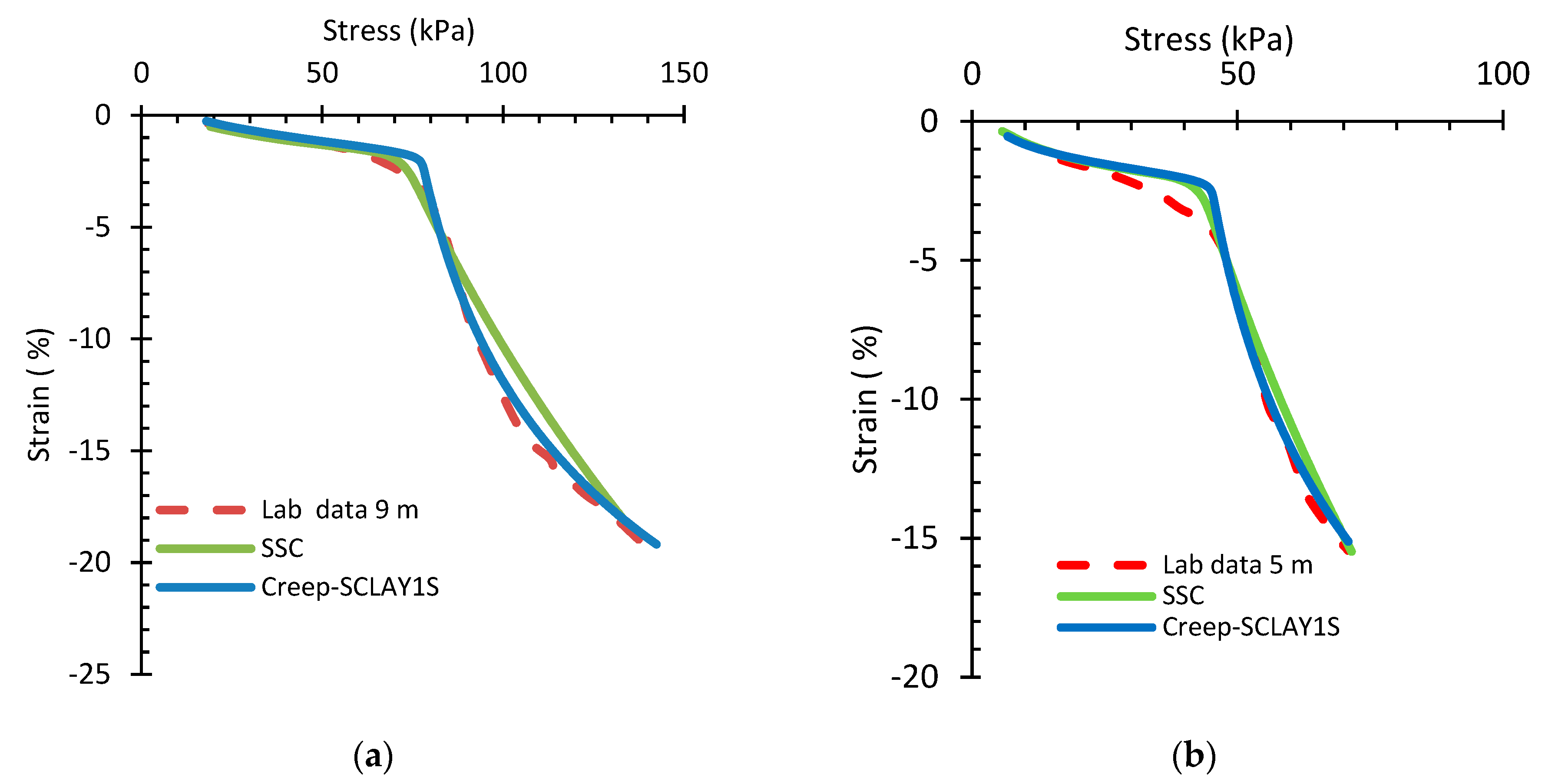
The results of the simulation are observable from SSC and Creep-SCLAY1S, as illustrated in Figure 3. The computed modified swelling index k* indicates a higher stiffness in the OC state, a phenomenon that may be attributed to sample disturbance; consequently, the value of k* was increased to align with laboratory results, despite the acknowledgment of the numerous uncertainties inherent in laboratory measurement.

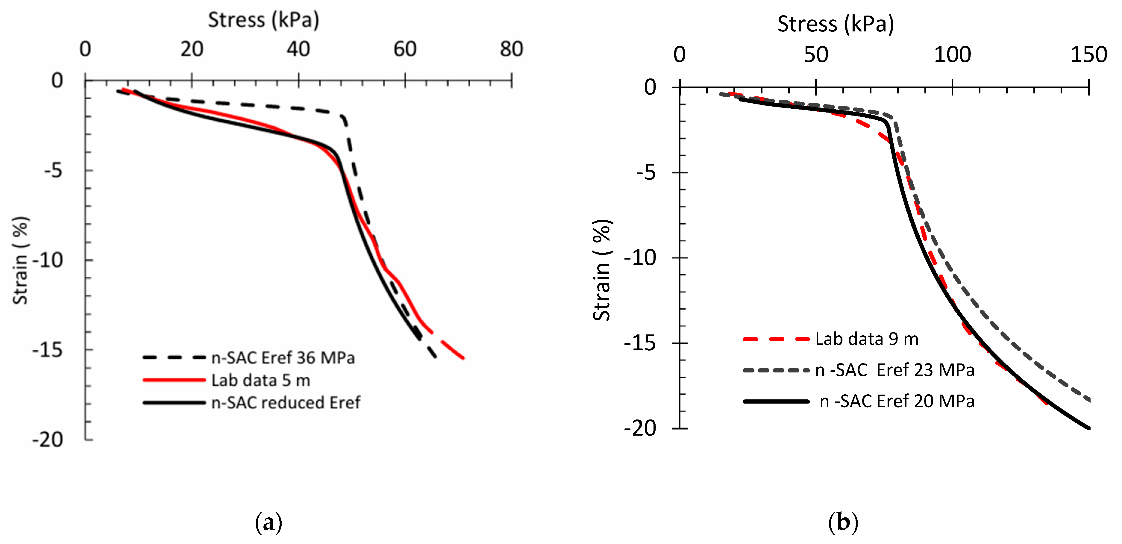
Figure 4 presents a comparison of CRS test simulations derived from n-SAC alongside laboratory measurements for depths of 5 m and 9 m within the soft clay layers. The calculated E^ref predicts an elevated stiffness, which subsequently diminishes. The E^ref value not only influences the soil stiffness in the OC state but also significantly affects the apparent preconsolidation pressure, thereby controlling the rate at which the soil is consolidated. In conclusion, the CRS tests and simulations utilizing the established soil parameters through the selected models effectively captured the stress–strain trajectory in a reasonably accurate manner.

Significant discrepancies were observed, particularly around the strain level of ε = 7% for the 5 m depth. In this region, both the SSC and Creep-SCLAY1S models begin to diverge from the measured stress–strain trajectory. This can be attributed to the limitations in capturing post-yield hardening behavior and potential destructuration effects, which become more pronounced at higher strain levels. For the 9 m depth, an underestimation of the yield stress was observed across all models, particularly in SSC, which may result from an inaccurate initial OCR or the inability of the model to fully simulate the time-dependent stiffness degradation due to creep.

These discrepancies highlight the need to go beyond a general conclusion and examine parameter sensitivities more thoroughly. While base parameters such as λ*, κ*, and μ* were calibrated, secondary parameters, such as the rate of structure loss (ω), rate of rotation (r_s), and the initial bonding ratio, play a crucial role in reproducing non-linear responses at large strains. Inadequate representation or calibration of these parameters can lead to mismatches in predicted versus observed behavior, especially near and beyond yield.

A more detailed sensitivity analysis was conducted post hoc to examine the influence of these advanced parameters. The results indicate that the Creep-SCLAY1S and n-SAC models are particularly sensitive to μ* and ω, which govern the magnitude and rate of creep-induced settlement and pore pressure buildup. Similarly, changes in the plastic hardening modulus and anisotropic rotational parameters significantly influence the slope of the stress–strain curve post-yield. These insights are elaborated in the supplemental section, where each model’s behavioral response is explored through parametric variation.

Thus, while the models captured the general trend of stress–strain behavior, especially in the normally consolidated range, the observed deviations at large strains underscore the importance of robust calibration and highlight the limits of simplified parameter sets. These observations enhance the technical contribution of the study and provide guidance for improving the practical use of advanced constitutive models in soft clay applications.

2.5. Finite Element Calculations

2.5.1. Finite Element Model

To conduct a numerical analysis utilizing PLAXIS 2D, an axis-symmetric model has been constructed, measuring 50 m in the x-axis direction and 14 m in the y-axis direction. The boundary conditions have been established in accordance with the standard fixities prescribed by PLAXIS. The hydraulic conditions have been set to incorporate two-sided drainage at both the top and bottom, while the left boundary has been sealed to maintain symmetry. The mesh generated can be seen in Figure 5, where the global coarseness has been selected as fine. Additionally, certain clusters, particularly those situated beneath the embankment, have been locally refined to ensure that the meshes are sufficiently accurate to yield acceptable numerical solutions.

2.5.2. Computation Process

The computation process involves determining initial in situ stresses based on K₀, followed by a construction phase lasting 25 days, during which the embankment is constructed. Subsequently, a consolidation phase is executed for durations of 21 years, 32 years, and 57 years.

Table 5. Applied steps during the calculation phases of PLAXIS.

Phase	Calculation Type	Stage Construction Time (Days)	Cumulative Time (Days)	Comments
Initial	K0-procedure	-	-	To create the in situ stress state
1	Consolidation	25	25	Construction of embankment
2	Consolidation	7665	7690	Consolidation until 21 years
3	Consolidation	4015	11,705	Consolidation until 32 years
4	Consolidation	9125	20,830	Consolidation until 57 years

presented below delineates the various calculation phases alongside their corresponding analysis procedures. The phreatic level has been positioned at 0.8 m beneath the ground level. To account for the impacts of hydraulic uplift resulting from the settlement of fill beneath the water table, the consolidation analysis has been conducted utilizing an updated mesh.

2.5.3. Finite Element Calculation Output

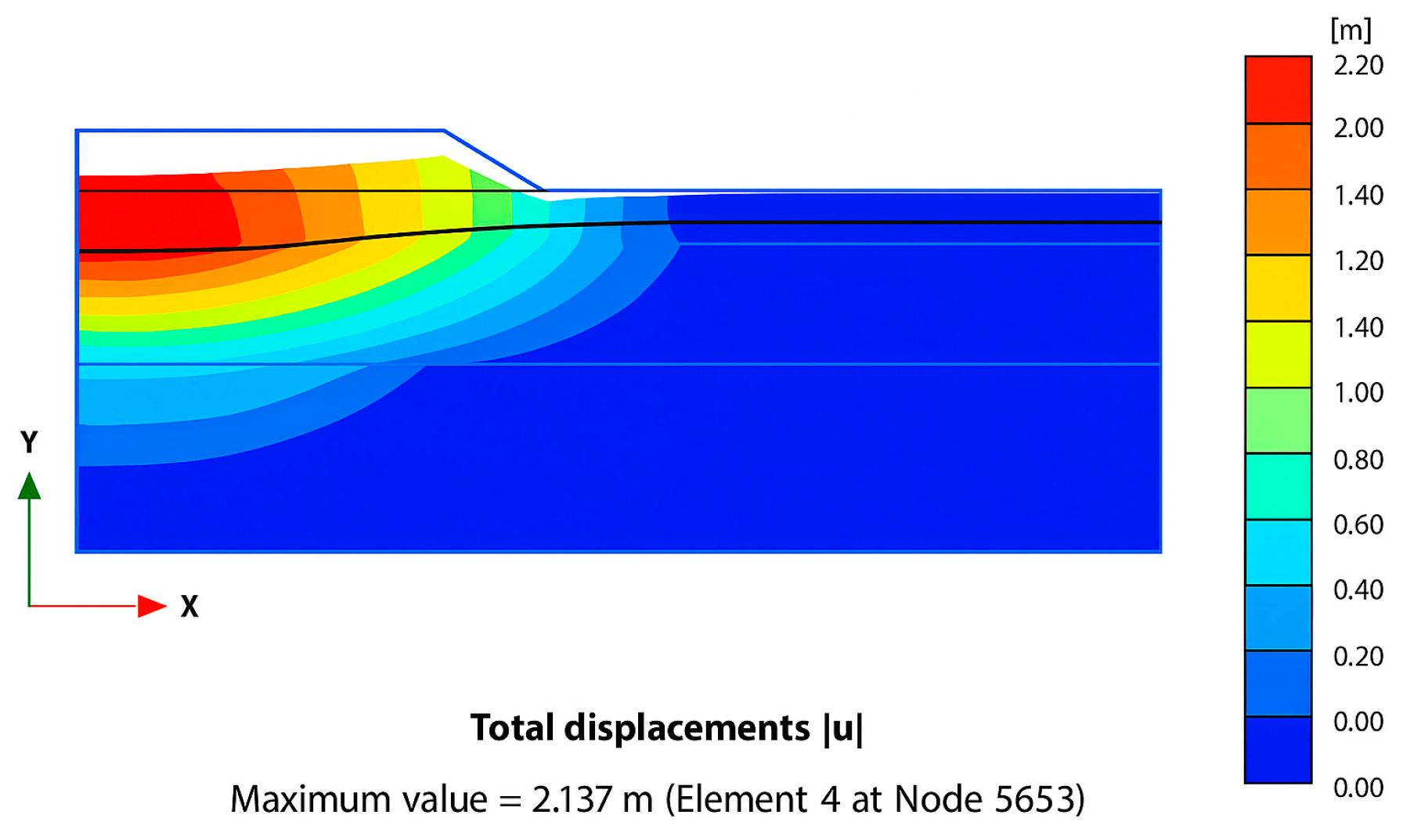
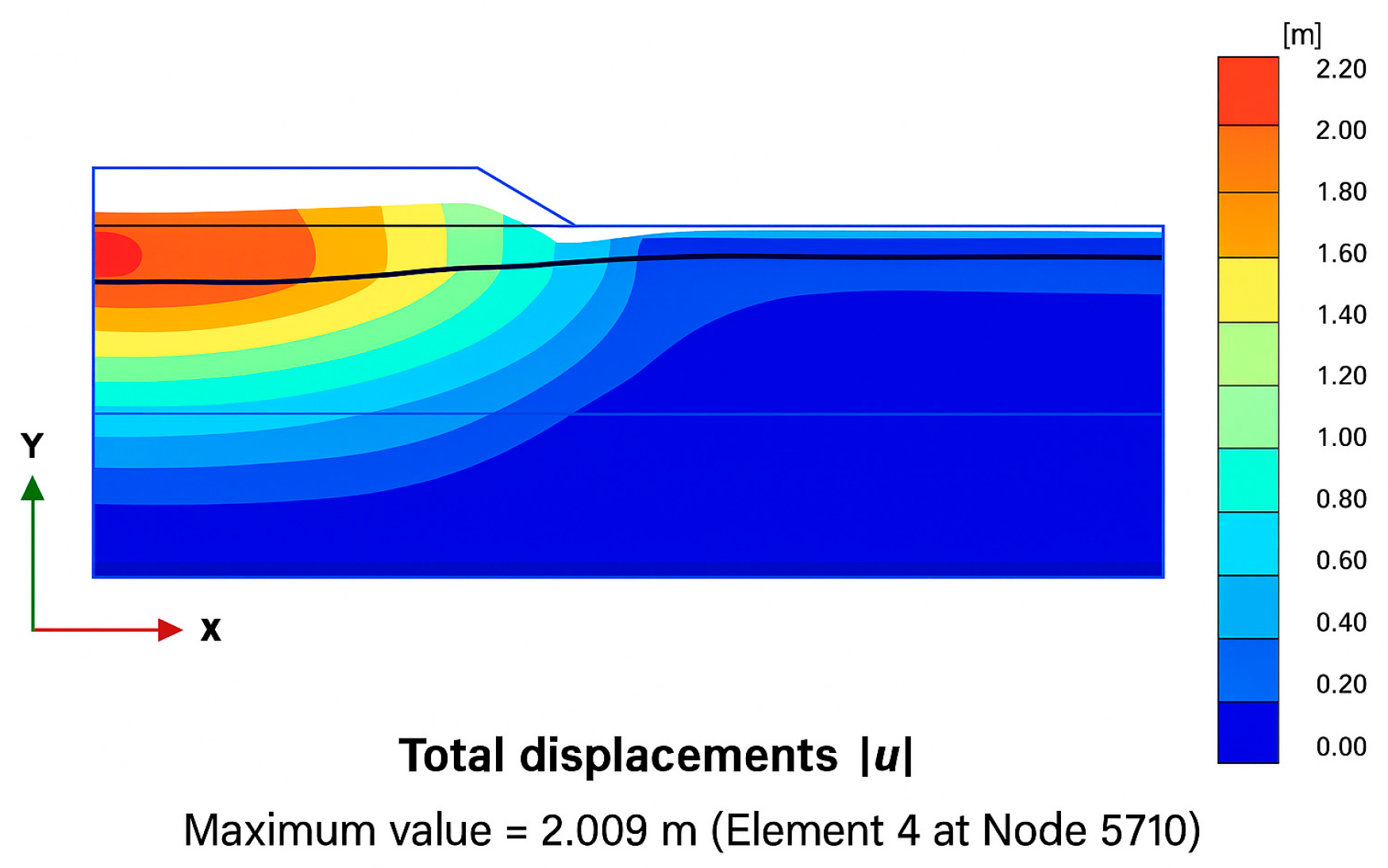
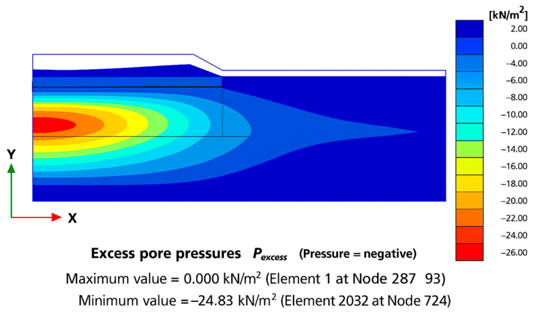
After doing the consolidation analysis for different consolidation phases, as in Table 5, from selected models, output figures have been obtained displaying the total displacement. The pore water pressure can be seen in Figure 6 and Figure 7, which depict the total vertical consolidation settlements of 2.13 m and 2.0 m, respectively, achieved with the n-SAC and SSC models after 57 years of embankment consolidation. Similarly, Figure 8 shows the maximum PWP obtained with the SSC model after 21 years of consolidation. The red area located at the top of the embankment signifies the greatest magnitude of displacement. The figure further indicates that significant displacements are concentrated beneath the center of the embankment. The various results derived from the calculations are elucidated in the subsequent section.

3. Results

The assessment encompasses the temporal measurements of settlement at various depths, the resultant excess pore water pressure over a span of years, and the vertical distribution of the settlement concerning depth.

3.1. Vertical Settlement

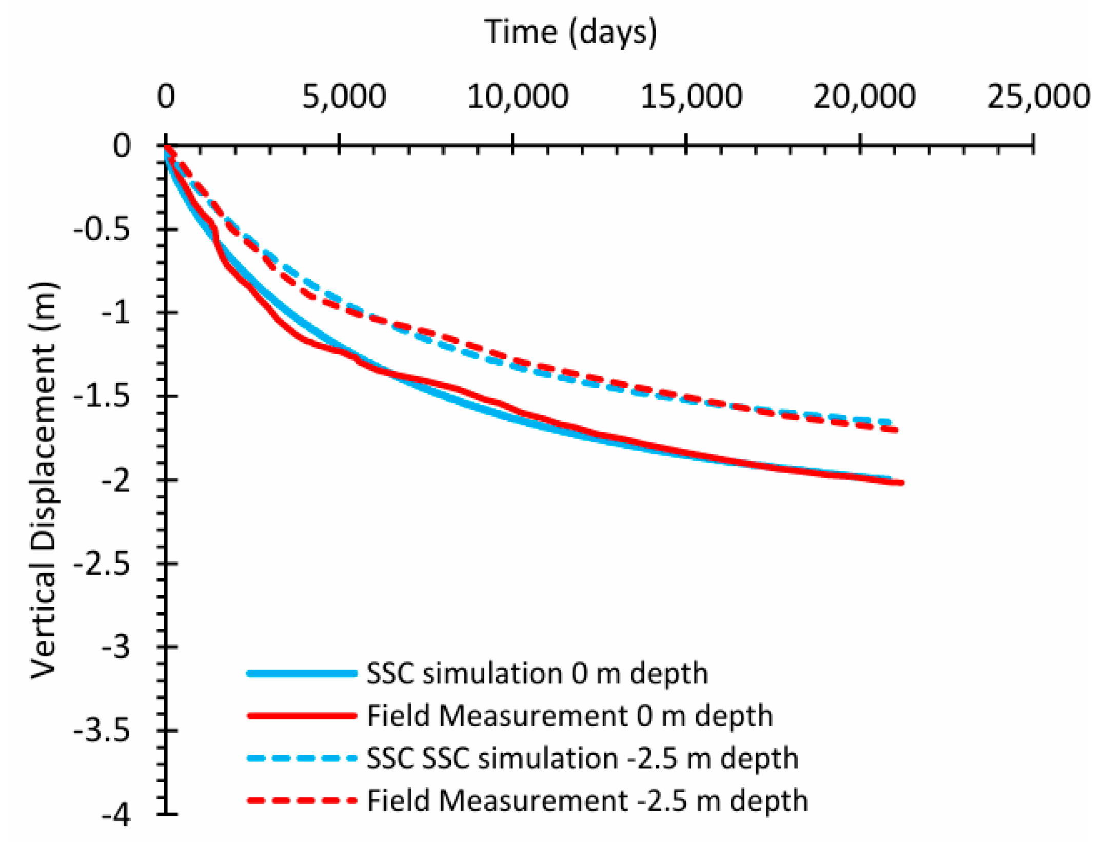
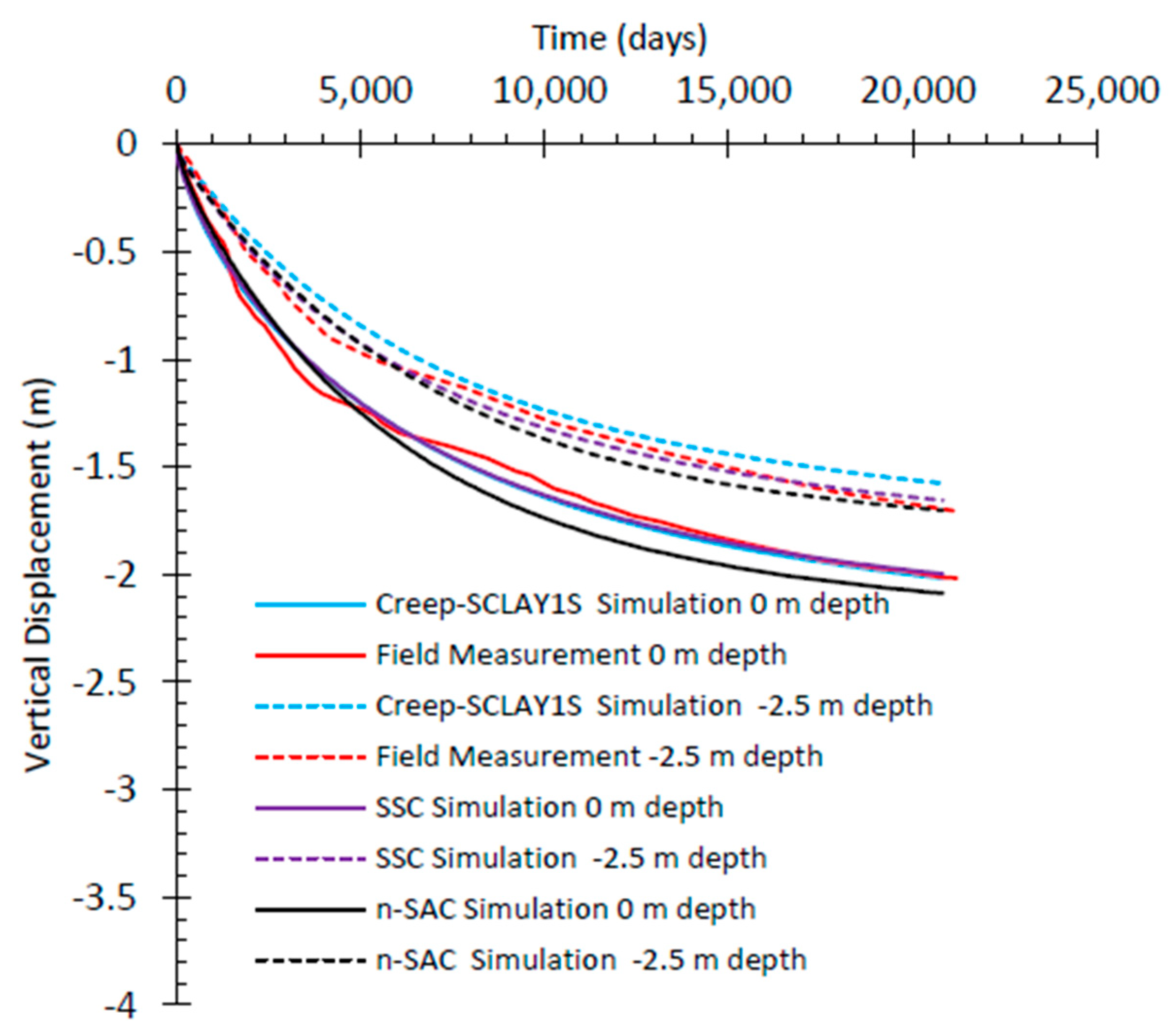
As elucidated in Section 2, temporal settlement measurements have been conducted over a period of 57 years following the construction of the embankment. The extent of the observed settlement at the center beneath the embankment across various depths, as derived from the SSC model, is depicted in Figure 9. The SSC model demonstrates a commendable proficiency in capturing settlement at the surface (0 m depth); however, at a depth of −2.5 m, it yields a comparatively lower prediction, as distinctly illustrated in Figure 9.

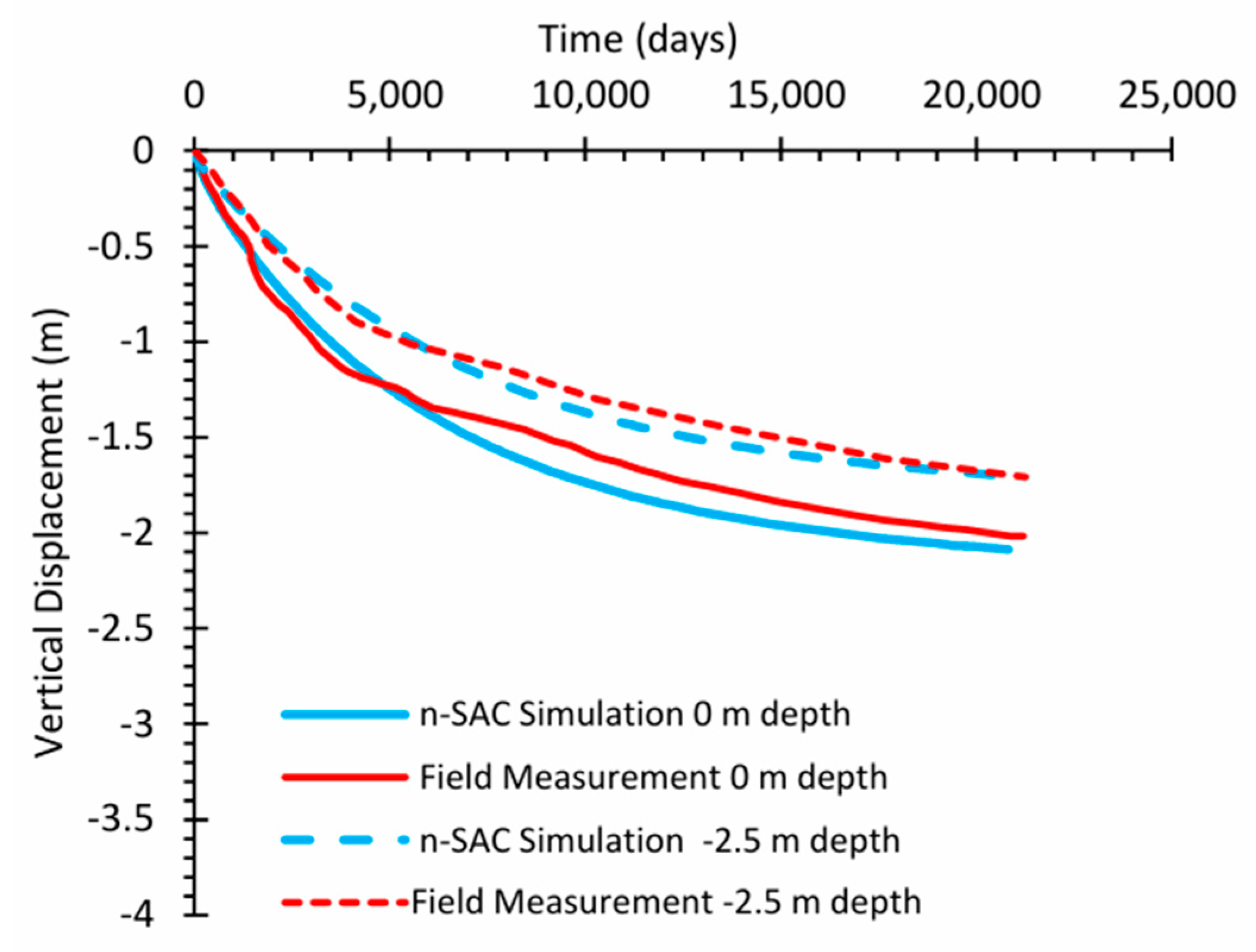
As illustrated in Figure 10, the n-SAC model is also adept at accurately capturing long-term settlement at a depth of −2.5 m, albeit it presents a slightly elevated value of approximately 2.11 m in contrast to the field measurement of 2.02 m; nonetheless, it is evident that n-SAC is proficient for long-term settlement assessments. This phenomenon may be attributable to the incorporation of novel features such as anisotropy and destructuration within the n-SAC model, which are prevalent in soft soil conditions.

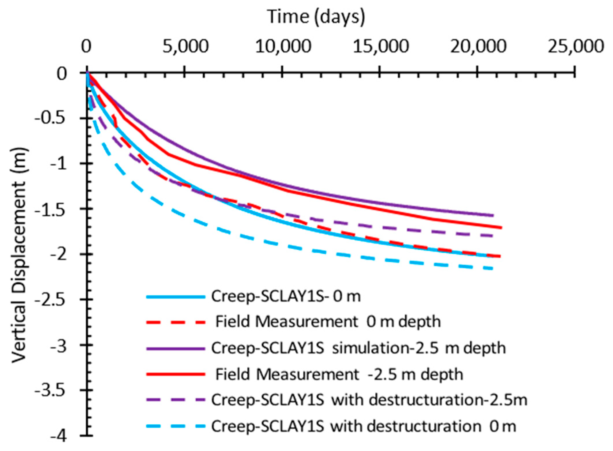
The Creep-SCLAY1S model has been executed in two distinct manners: one involving the setting of the destructuration parameter to zero, and the other incorporating destructuration. While using the parameters χ⁰, ξ, and ξ_d, which are related to destructuration in the Creep-SCLAY1S model, λ* is replaced with the intrinsic value, which is λ_i*. However, due to the lack of data for remolded samples, the slope of the intrinsic compression line, λ_i*, which is much lower than λ*, could not be estimated properly. As indicated in Figure 11, the Creep-SCLAY1S model was also capable of effectively capturing settlement without the inclusion of destructuration; however, when employing the destructuration parameter, it yields a value that is marginally higher than that of n-SAC, approximately 2.14 m compared to the 2.02 m field measurement, which may be ascribed to inaccuracies in the sensitivity measurements employed to compute the initial bounding value χ⁰.

Although n-SAC is conceptually more advanced, its performance lagged behind SSC due to the limited calibration data for complex parameters. SSC performed better due to its empirical tuning and simpler structure. We now emphasize that model complexity must be matched with high-quality data and robust calibration to realize its potential. This limitation and our contribution are clearly stated.

While the n-SAC model is theoretically more advanced due to its ability to simulate anisotropy, destructuration, and non-associated flow behavior, its performance in the simulation of long-term settlement in Figure 10 appears to be less aligned with the field observations than that of the simpler SSC model. This outcome, though initially counterintuitive, can be attributed to multiple factors.

First, the parameters used for the n-SAC model were largely adopted from literature sources and SGI reports, due to the limited availability of detailed experimental data, particularly regarding advanced bonding and structural degradation parameters. These include the rate of rotation (ω), time resistance number (r_s), and initial bonding ratio, which significantly affect creep and settlement responses but are difficult to determine without specialized laboratory testing.

Second, unlike the SSC model, which relies on fewer, well-understood parameters, n-SAC’s higher complexity demands a more rigorous calibration process. In the present study, a trial-based approach was used for parameter selection, which may have introduced calibration limitations. The better fit of SSC with the field data may thus reflect the advantage of empirical tuning over theoretical sophistication in the absence of robust, site-specific data for advanced models.

Recognizing this, a post hoc sensitivity analysis and optimization attempt were conducted for n-SAC. It revealed that small variations in structural and creep parameters could produce significant deviations in long-term settlement predictions. Therefore, the relatively weaker performance of n-SAC does not undermine the model’s conceptual strength but rather emphasizes the importance of well-designed experimental programs and advanced parameter calibration techniques, such as inverse modeling or numerical optimization, which were beyond the scope of the current dataset.

This observation supports the conclusion that model complexity must be matched with data quality and calibration effort to fully realize predictive accuracy in practical applications.

3.2. Settlement with Depth

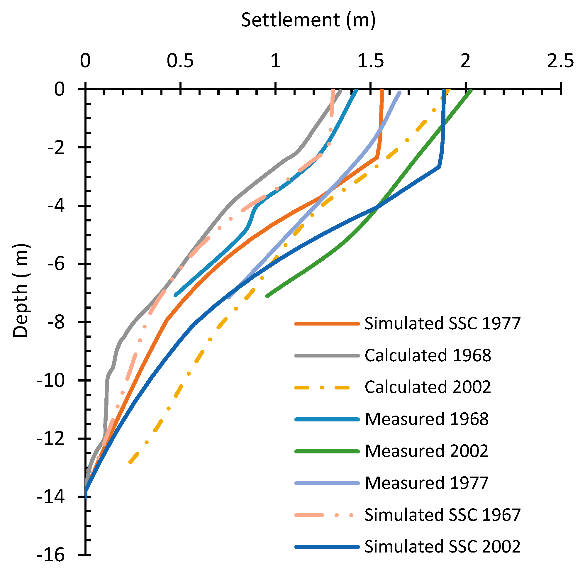
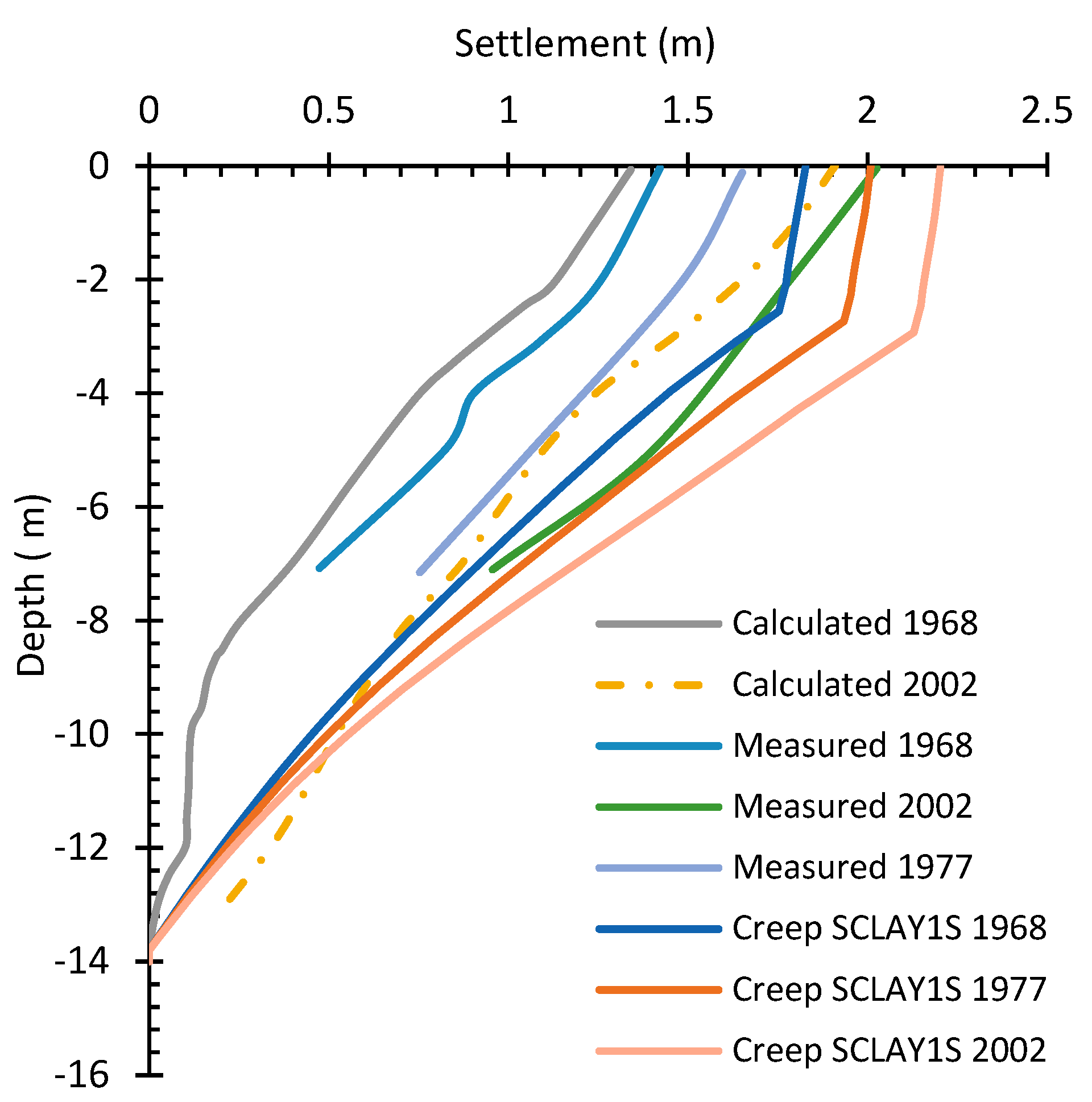
Figure 12, Figure 13 and Figure 14 delineate a comparative analysis of the simulated results from the SSC, Creep-SCLAY1S, and n-SAC models following 21, 32, and 57 years of consolidation, in conjunction with the measured and calculated vertical displacement profiles along the center of the embankment, respectively. There are two in situ measured values, one derived from installed markers and the other from variations in water content. All employed models demonstrate the capability to effectively capture the overall distributions of settlement across different layers. Nevertheless, the SSC model predicts lower values in comparison to the other two models, while the predictions from the Creep-SCLAY1S model are the highest, with the most significant discrepancies observed in the settlement predictions for the upper soil layers.

3.3. Pore Pressure

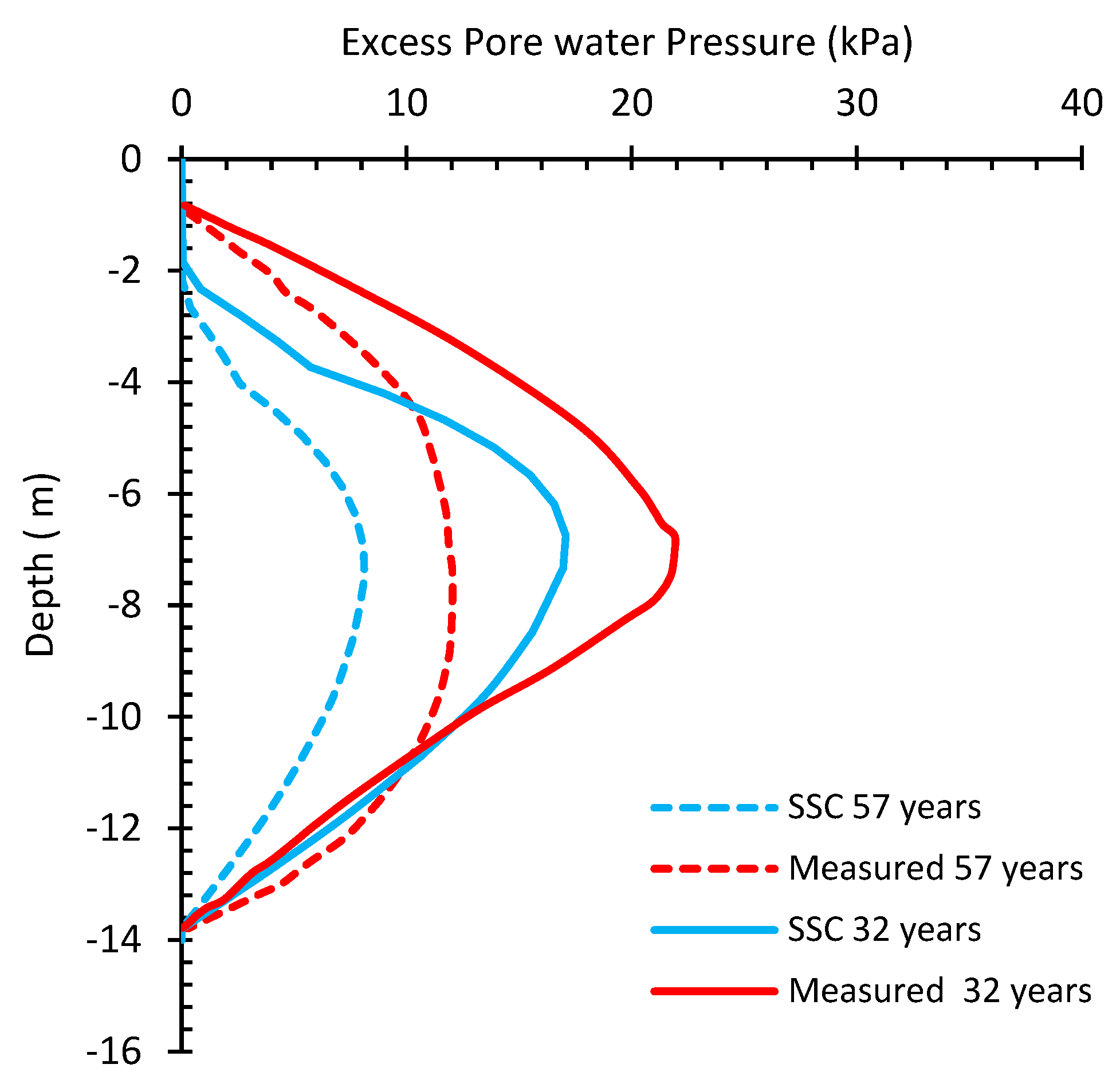
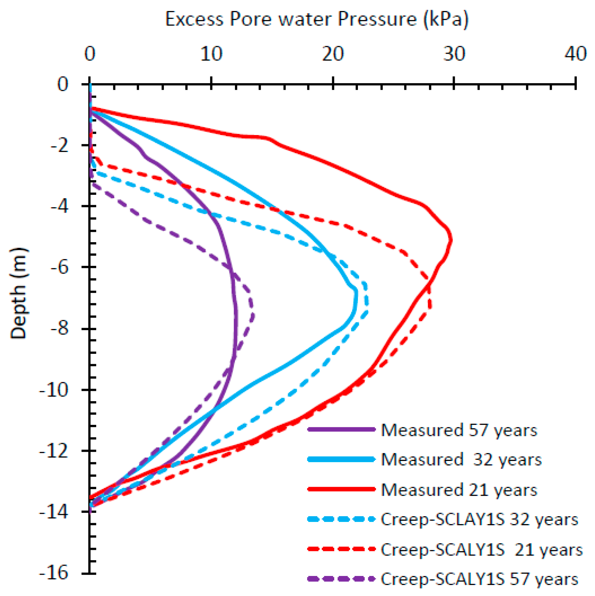
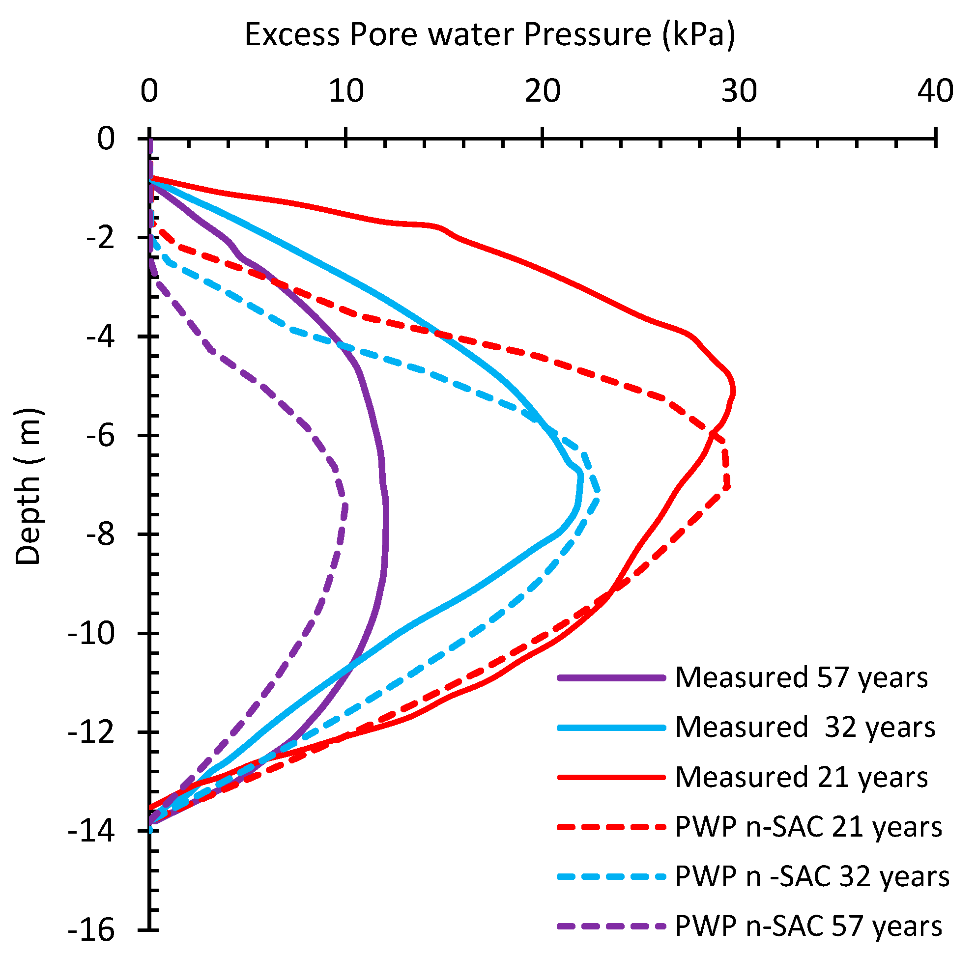
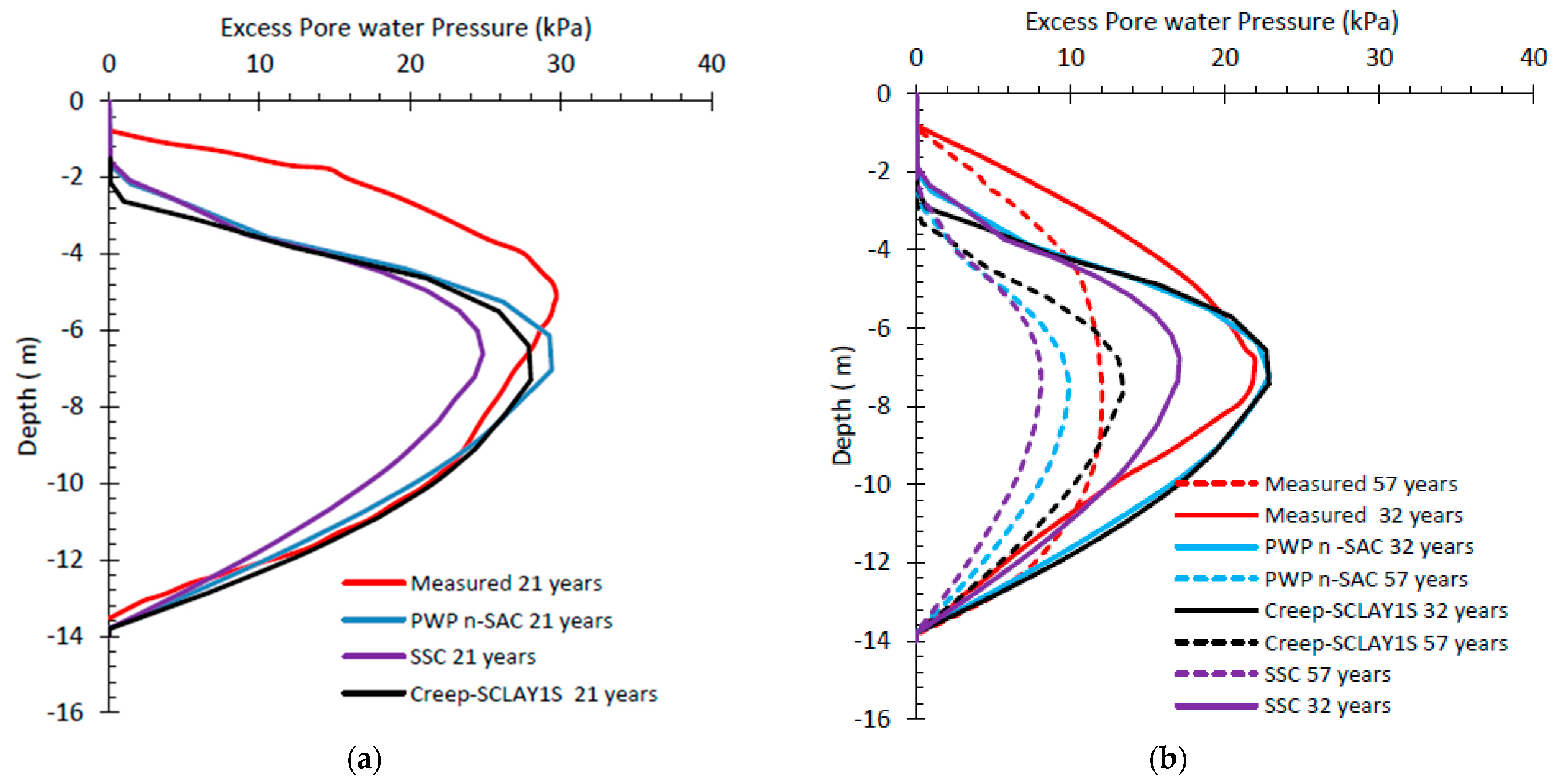
Figure 15, Figure 16 and Figure 17 illustrate the measured and computed distributions of excess pore pressure along the central axis of the embankment after 21, 32, and 57 years of consolidation. It has been noted that there may be some inaccuracies in the field measurements of excess pore pressure. Consequently, it is difficult to determine whether the models are making accurate or inaccurate predictions about the generated excess pore pressure.

The three models used showed the ability to predict the contour of excess pore pressure distribution, with the highest generated pore pressure found within the intermediate layers. Among the three models, the calculations from n-SAC and Creep-SCLAY1S are notably closer to the field measurements in comparison to those produced by SSC.

4. Discussion

As shown by Figure 9, Figure 10 and Figure 11 above, the time–settlement curves for all three models exhibit a strong resemblance, with the settlement recorded after 57 years measuring approximately 2 to 2.15 m, in contrast to the field result of 2.05 m. Figure 18 indicates that the settlement rates for Creep-SCLAY1S and n-SAC exceed that of SSC. This discrepancy may be attributed to the effects of anisotropy and destructuration [22,25,36].

A comparative analysis of Figure 12, Figure 13 and Figure 14 provides a comprehensive perspective on the vertical displacement profile along the center of the embankment following 21, 32, and 57 years of consolidation. Among the three models analyzed, SSC yields the lowest predictions, whereas Creep-SCLAY1S presents the highest estimates. Creep-SCLAY1S and n-SAC produce remarkably similar results, demonstrating increased settlement towards the upper regions of the clay layers, which may be influenced by anisotropic effects. Figure 15, Figure 16 and Figure 17 depict the distribution of excess pore pressure beneath the embankment after 21, 32, and 57 years. Furthermore, Figure 19 offers a comparison of the pore pressure responses from the models at various time intervals. The maximum pressure magnitude is observed in n-SAC, while predictions from the other models are relatively consistent; however, the distribution profiles distinctly indicate a maximum value at the center of the clay layers.

The models utilized are effective in capturing the long-term settlement of the embankment; however, some discrepancies remain between the final measured settlements and the predictions after 57 years, especially with Creep-SCLAY1S and n-SAC.

Based on the case study of the Lilla Mellösa test embankment, the SSC, n-SAC, and Creep-SCLAY1S models successfully capture the long-term settlement of the embankment, although notable discrepancies remain between the final measured settlements and predictions from Creep-SCLAY1S and n-SAC after 57 years. The n-SAC and Creep-SCLAY1S models incorporate additional attributes such as anisotropy and destructuration, distinguishing them from SSC, which are likely the principal factors contributing to the greater total settlements observed in the soil layers.

The n-SAC and Creep-SCLAY1S models exhibit commendable proficiency in accurately simulating the stress–strain behavior observed during CRS test simulations in comparison to the SSC model. Nevertheless, during field test simulations, these models forecast a greater degree of horizontal settlement than the SSC model, which may be attributed to the slope of the critical state line influencing the soil’s plasticity. The n-SAC and Creep-SCLAY1S models utilize the value of M derived from Jaky’s formula alongside a rotational yield surface, whereas the SSC model employs the value of M as per the modified Cam Clay theory. Consequently, these models hold significant value in scenarios where horizontal displacement is of paramount importance.

Finally, when considering various model characteristics such as the requisite number of input parameters and computational time, the SSC model emerges as a compelling option for predictions concerning soft soil. However, the n-SAC and Creep-SCLAY1S models may yield superior predictions compared to the isotropic SSC model, provided they are meticulously implemented with accurate parameters. As previously articulated, the identification of the various parameters relies heavily on empirical relationships. The input soil parameters are ascertained through a limited number of laboratory tests, and the impact of sample disturbances on the determination of parameters plays a significant role in the resulting calculations. Furthermore, the test site is considerably aged, thereby raising concerns regarding the reliability of the measuring instruments and methodologies employed, which may not yield precise results.

5. Conclusions

The n-SAC and Creep-SCLAY1S models have additional features like anisotropy [37] and destructuration [16] compared to the SSC model. These features are likely the primary factors contributing to the increased total settlements observed in soil layers, making them important for predicting long-term behavior. However, the n-SAC and Creep-SCLAY1S models necessitate the determination of several diverse parameters, the identification of which is not a straightforward endeavor. Due to insufficient data on remolded samples, the slope of the intrinsic compression line, λ_i*, is much lower than λ*, and could not be accurately estimated. It has also been noted that the efficacy of these models is highly sensitive to variations in this particular parameter.

Due to the lack of laboratory data for remolded (structureless) clay samples, the intrinsic compression slope λ_i*, which represents the compressibility of fully destructured soils and is typically much lower than the structured compression index λ*, could not be independently determined in this study. Acknowledging this limitation, the focus of the work shifts from resolving the intrinsic parameter gap to evaluating how different creep models respond to parameter assumptions in structured soft clays. Through a comparative simulation framework involving three advanced constitutive models—SSC, Creep-SCLAY1S, and n-SAC—under a common benchmark case, this study systematically demonstrates the sensitivity of model outputs to structural and creep-related parameters, even when complete laboratory data are unavailable. This research contributes to the geotechnical modeling field by highlighting the influence of parameter unavailability on model reliability, providing a structured framework for comparative model evaluation under realistic site conditions, and offering practical guidance for parameter prioritization and model selection in data-scarce environments. Further research involving targeted sampling of remolded specimens and advanced laboratory testing is recommended to improve the accuracy of intrinsic parameter estimation and refine model calibration practices.

In practice, it is difficult to identify equivalent soil parameters for all three models, with considerable uncertainty in determining the destructuration parameter ω and the intrinsic creep number r_si. Although these models can simulate settlement and pore pressure, using back-calculated parameters from field measurements introduces uncertainty. With careful use and strong support from accurate lab and field data, the n-SAC and Creep-SCLAY1S models may offer more reliable results than the simpler, isotropic SSC model.