Abstract
Geotechnical engineering relies heavily on predicting soil strength to ensure safe and efficient construction projects. This paper presents a study on the accurate prediction of soil strength properties, focusing on hydrated-lime activated rice husk ash (HARHA) treated soil. To achieve precise predictions, the researchers employed two grey-box machine learning models—classification and regression trees (CART) and genetic programming (GP). These models introduce innovative equations and trees that readers can readily apply to new databases. The models were trained and tested using a comprehensive laboratory database consisting of seven input parameters and three output variables. The results indicate that both the proposed CART trees and GP equations exhibited excellent predictive capabilities across all three output variables—California bearing ratio (CBR), unconfined compressive strength (UCS), and resistance value (Rvalue) (according to the in-situ cone penetrometer test). The GP proposed equations, in particular, demonstrated a superior performance in predicting the UCS and Rvalue parameters, while remaining comparable to CART in predicting the CBR. This research highlights the potential of integrating grey-box machine learning models with geotechnical engineering, providing valuable insights to enhance decision-making processes and safety measures in future infrastructural development projects.
1. Introduction
Soil stabilization techniques play an important role in geotechnical engineering to improve the engineering properties of weak or problematic soils [1]. Traditional methods, such as soil replacement or compaction, have limitations in terms of cost, implementation, and environmental impact [2,3]. As a sustainable and economical alternative, soil stabilization using supplementary materials/additives has attracted considerable attention. One of these approaches includes adding hydrated lime and rice husk ash to the soil [4].
Because of its unique properties, hydrated lime is a widely used additive in soil stabilization [4,5]. It is a fine, white powder obtained from the hydration of quicklime (calcium oxide) and consists mainly of calcium hydroxide [4,5]. When hydrated lime is added to soil, it undergoes chemical reactions with clay minerals, which lead to reduced soil compressibility, improved shear strength, and increased durability [4,5,6]. These reactions, known as cation exchange and pozzolanic reactions, lead to the formation of stable compounds that bind soil particles together [4,5,6].
Rice husk ash (RHA), a byproduct of the rice milling industry, is also promising as an additive in soil stabilization [7]. RHA is obtained by burning rice husks at high temperatures, which converts the organic matter into amorphous silica and other inorganic components [8]. When added to soil, RHA acts as a pozzolanic agent and reacts with calcium hydroxide from hydrated lime to form additional cementitious compounds [4,5]. The inclusion of RHA in the soil stabilization process further improves the strength, stiffness, and durability of the stabilized soil [9]. Utilizing rice husk ash in cement and concrete offers numerous advantages, including reduced heat of hydration, improved strength, decreased permeability at higher dosages, enhanced resistance to chloride and sulfate, cost savings through reduced cement usage, and environmental benefits by mitigating waste disposal and lowering carbon dioxide emissions [10,11,12,13,14,15,16,17]. Jafer et al. [18] focused on developing a sustainable ternary blended cementitious binder (TBCB) for soil stabilization. TBCB incorporates waste materials and improves the engineering properties of the stabilized soil. The results showed a reduced plasticity index and increased compressive strength. XRD and SEM analyses confirmed the formation of cementitious products, leading to a solid structure. TBCB offers a promising solution for soil stabilization with a reduced environmental impact [18].
The combination of hydrated lime and rice husk ash has synergistic effects in soil stabilization [19,20]. The pozzolanic reactions between these materials and the soil matrix contribute to the development of cementitious compounds, thereby increasing strength and reducing permeability [21]. In addition, the incorporation of rice husk ash contributes to the utilization of an agricultural waste product and increases sustainability in construction practices [22,23].
The success of soil stabilization using hydrated lime and rice husk ash depends on various factors such as the type and properties of the soil, dosage and ratio of supplementary materials/additives, curing conditions, and testing methods used [24,25]. Accurate predictive models that consider these parameters can help optimize the stabilization process and ensure the desired engineering performance of treated soils [25,26]. The accurate prediction of soil strength performance is crucial for geotechnical engineering. Artificial intelligence (AI) methods, including ANN, SVM, ANFIS, CNN, LSTM, decision trees, and GPR, have been applied in various geotechnical applications [27,28,29,30]. ANN is the most widely used AI technique, contributing to improved predictions and optimizations in geotechnical engineering [27]. These AI methods enhance understanding and decision-making in areas such as frozen soils [31,32,33], rock mechanics [34,35,36], slope stability [37,38,39], soil dynamics [40,41,42,43,44], tunnels [45,46,47], dams [48,49,50], and unsaturated soils [51,52,53]. Onyelowe et al. [25] used artificial neural network (ANN) algorithms to predict the strength parameters of expansive soil treated with hydrated-lime activated rice husk ash. The algorithms performed well, with the Levenberg−Marquardt Backpropagation (LMBP) algorithm showing the most accurate results. The predicted models had a strong correlation coefficient and a high performance index.
AI algorithms aimed at material characterization and design have faced doubt because people are worried about the opacity and reliability of their intricate models [54]. The primary obstacle is the absence of transparency and methods to extract knowledge from these models [54]. There are different categories of mathematical modeling techniques: white-box, black-box, and grey-box, each varying in their level of transparency [54,55]. White-box models are grounded in fundamental principles and can elucidate the underlying physical relationships within a system [54,55,56]. On the other hand, black-box models lack a clear structure, making it difficult to understand their inner workings [54,55,56]. Grey-box models fall in between, as they identify patterns in data and offer a mathematical structure for the model [54,55,56]. Artificial neural networks (ANN) are well-known examples of black-box models in engineering [57]. Although they are widely used, they lack comprehensive information about the relationships they establish. In contrast, genetic programming (GP) and classification and regression trees (CART) are newer grey-box modeling techniques that employ an evolutionary process to develop explicit prediction functions and trees, respectively, making it more transparent compared to black-box methods such as ANN. GP and CART models provide valuable insights into system performance as they offer mathematical and tree structures, respectively, that aid in understanding the underlying processes. They have shown promise in terms of accuracy and efficiency across various applications. Here are the benefits of AI-based grey-box models:
- -
- Transparency with Structure: Grey-box models, such as genetic programming (GP) and classification and regression trees (CART), strike a balance between white-box and black-box models. They offer transparency by identifying data patterns while providing a clear mathematical or tree-based structure, making it easier to understand the model’s operations [58].
- -
- Enhanced Insights: The structured nature of grey-box models allows for a deeper understanding of the underlying processes. Unlike black-box models such as artificial neural networks (ANN), GP and CART provide insights into system performance through their explicit prediction functions and tree structures.
- -
- Transparency in Evolution: Techniques such as genetic programming (GP) use an evolutionary process to develop prediction functions, making the model’s development and evolution more transparent. This transparency aids in tracking the model’s progress and understanding its decision making [59].
- -
- Accuracy and Efficiency: Grey-box models, including GP and CART, have demonstrated promise across various applications, offering a combination of accuracy and efficiency. Their transparency, coupled with the ability to capture complex relationships in data, makes them valuable tools for mathematical modeling in engineering and other fields.
Based on the literature review provided, this research is groundbreaking in its systematic application of two distinct grey-box artificial intelligence models: genetic programming (GP) and classification and regression tree (CART). These models are utilized for the first time to predict critical soil parameters—California bearing ratio (CBR), unconfined compressive strength (UCS), and resistance value (Rvalue) determined through in-situ cone penetrometer tests—for expansive soil treated with recycled and activated rice husk ash composites. The study further evaluates the significance of input parameters, performing a sensitivity analysis on 121 datasets, each consisting of seven inputs: hydrated-lime activated rice husk ash (HARHA), liquid limit (LL), plastic limit (PL), plasticity index (PI), optimum moisture content (wOMC), clay activity (AC), and maximum dry density (MDD). HARHA, a material produced by blending 5% hydrated lime with rice husk ash, acts as an activator, and it is created from the controlled combustion of rice husk waste. Different proportions of HARHA (ranging from 0.1% to 12% in increments of 0.1% of weight) were employed to treat clayey soil, with the resulting effects on soil properties meticulously examined and documented within the study.
2. Database Processing
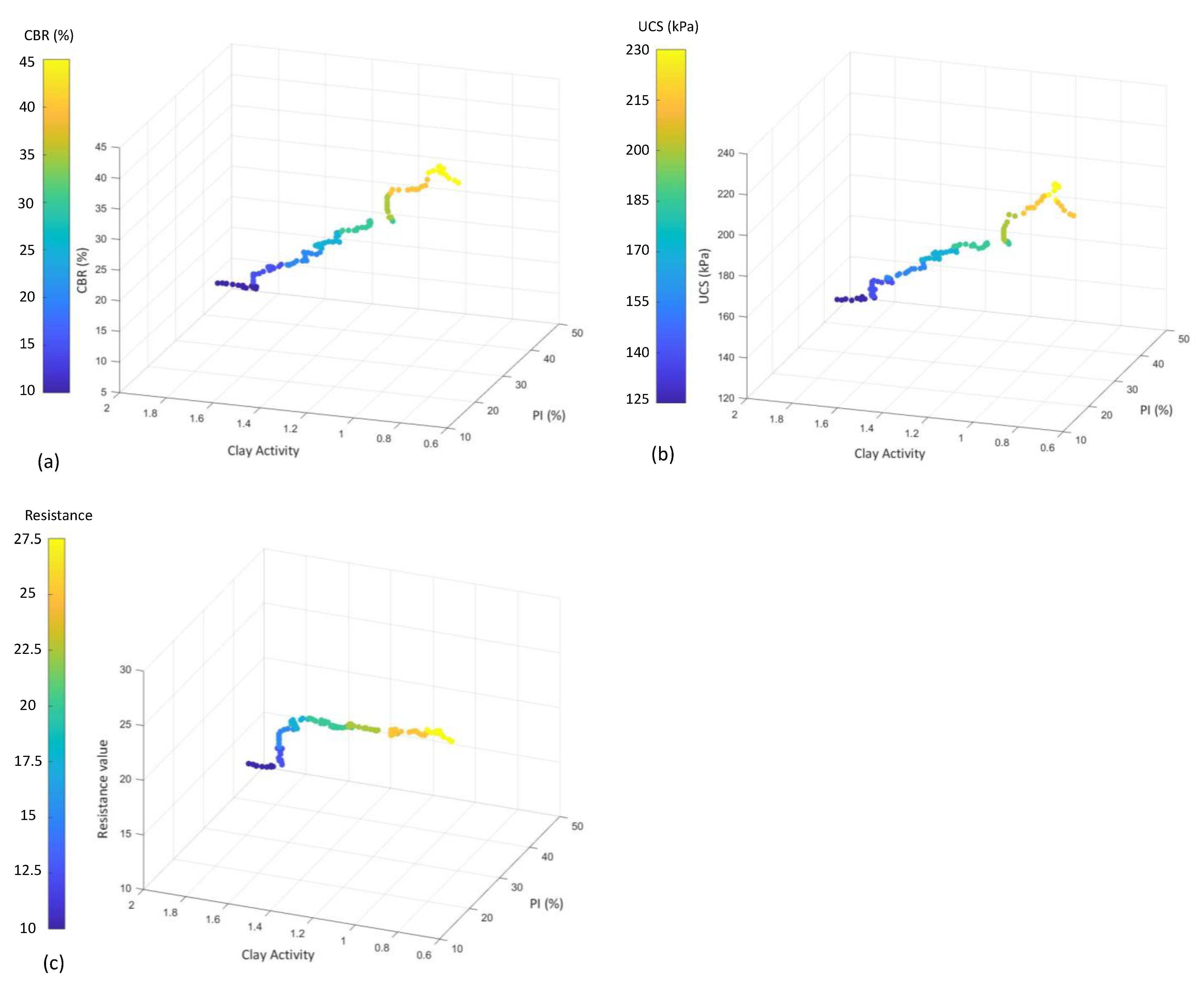
This study uses a 121-laboratory database, originally studied by Onyelowe et al. [25], who examined expansive clays by conducting tests on both untreated and treated soils to determine the datasets by observing the effects of stabilization on the predictor parameters. Onyelowe et al. [25] conducted a series of tests utilizing a laboratory to gather the data. The database is represented as three-dimensional diagrams in Figure 1. Experiments were conducted on expansive clay soil, both untreated and treated with hydrated-lime activated rice husk ash (HARHA). The HARHA, a binder developed by blending rice husk ash with hydrated lime, was tested at varying proportions on the clayey soil.
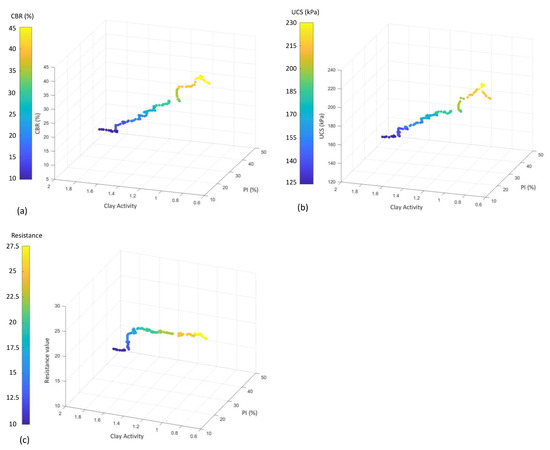
Figure 1.
Distribution of the database used based on (a) CBR, (b) UCS, and (c) resistance values.
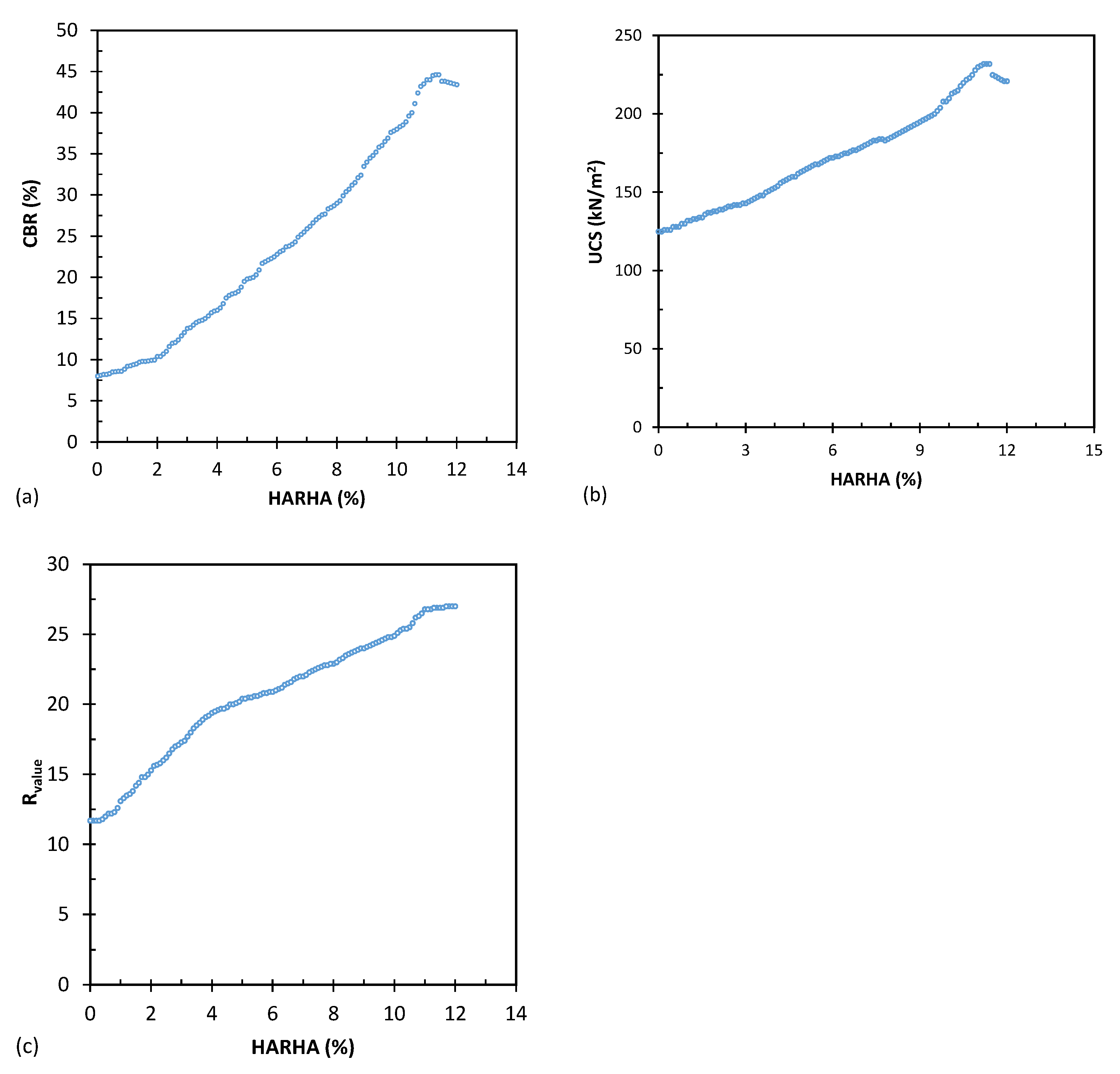
Figure 2 depicts the effect of adding HARHA on three parameters: CBR, UCS, and resistance values. The results indicate that all three parameters increased with the percentage of additive until they reached a peak. Afterward, they showed slight decreases. An approximate value of 11.5% could be considered the optimal amount of HARHA additive.
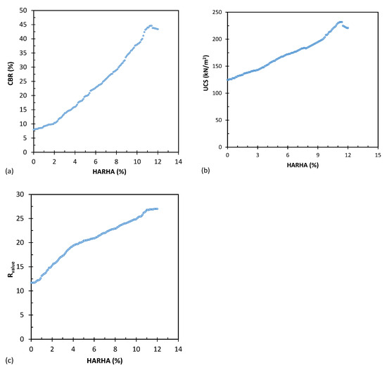
Figure 2.
Effect of HARHA on (a) CBR, (b) UCS, and (c) resistance values.
The existing database contained seven inputs, which were as follows: hydrated-lime activated rice husk ash (HARHA), liquid limit (LL), plastic limit (PL), plasticity index (PI), optimum moisture content (wOMC), clay activity (AC), and maximum dry density (MDD). The plasticity index parameter was derived by subtracting the liquid limit from the plastic limit, while the remaining parameters were independent and lacked a direct correlation.
This database is noteworthy for using one of the largest sources of laboratory-derived UCS, CBR, and Rvalue measurements documented in the literature, boasting a considerable number of entries, totaling seven.
Table 1 shows the statistical characteristics of the database utilized in this study, presenting the minimum, maximum, and mean values for both inputs and outputs. These descriptive statistics offer valuable insights into the distribution and properties of the data, providing crucial information for model selection and optimization in subsequent analyses.

Table 1.
Descriptive statistics for the collected database.
2.1. Outliers
Within the realm of database preparation, a pivotal concern revolves around the detection of outliers. Within a database context, an outlier denotes a data point that exhibits notable deviation from the majority of the data points [60,61]. The imperative lies in identifying and outrightly excluding these data points from the modeling process, as they have the potential to lead the model astray. Recognizing these particular data instances constitutes a pivotal stride in statistical analysis, commencing with the description of normative observations [62,63,64]. This entails an overarching evaluation of the graphed data’s configuration, with the identification of extraordinary observations that diverge significantly from the data’s central mass—termed outliers.
Two graphical techniques commonly used to identify outliers are scatter plots and box plots [54,65]. The latter utilizes the median, lower quartile, and upper quartile to display the data’s behavior in the middle and at the distribution’s ends. Furthermore, box plots employ fences to identify extreme values in the tails of the distribution. Points beyond an inner fence are considered mild outliers, while those beyond an outer fence are regarded as extreme outliers [54,66,67].
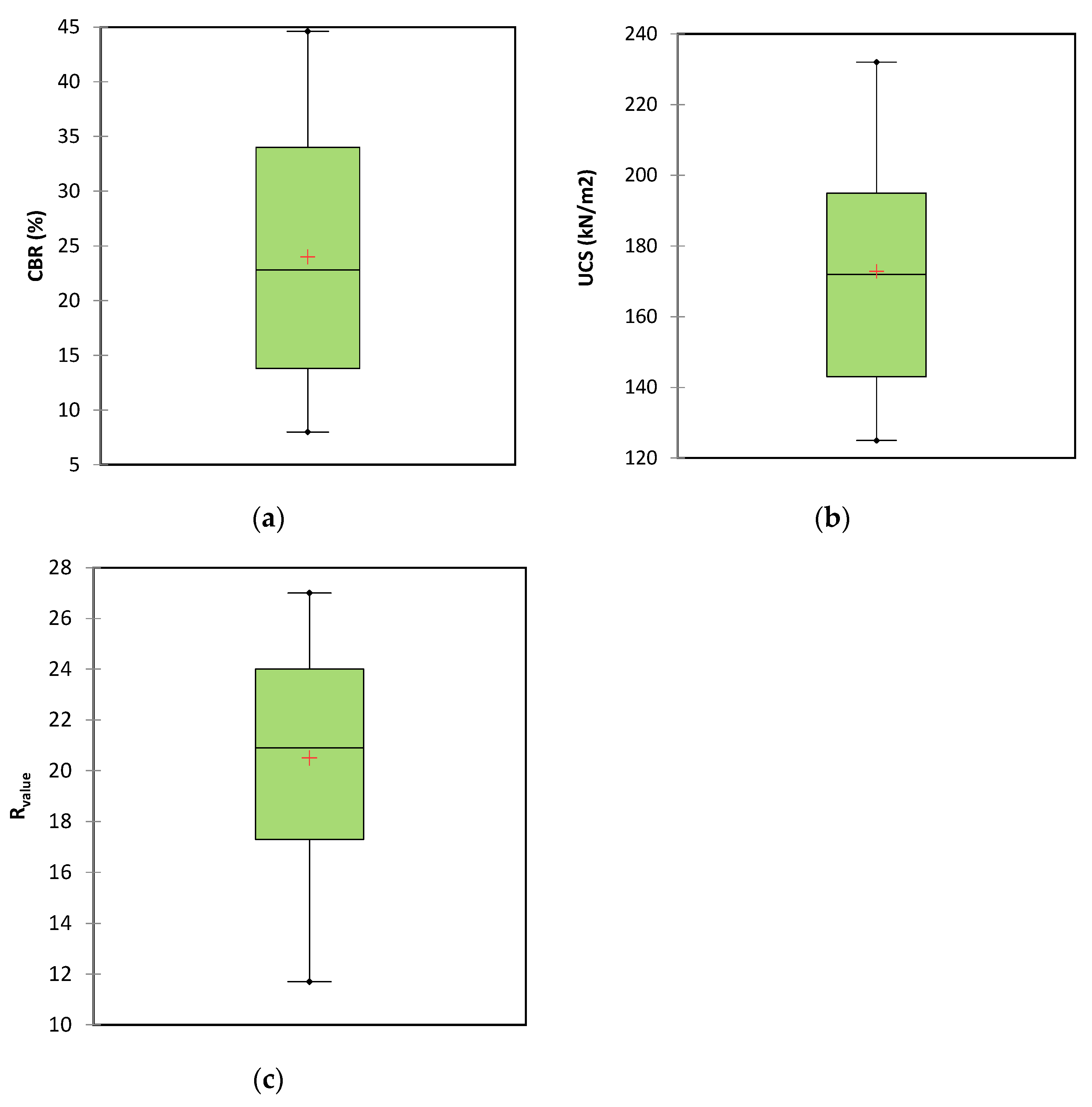
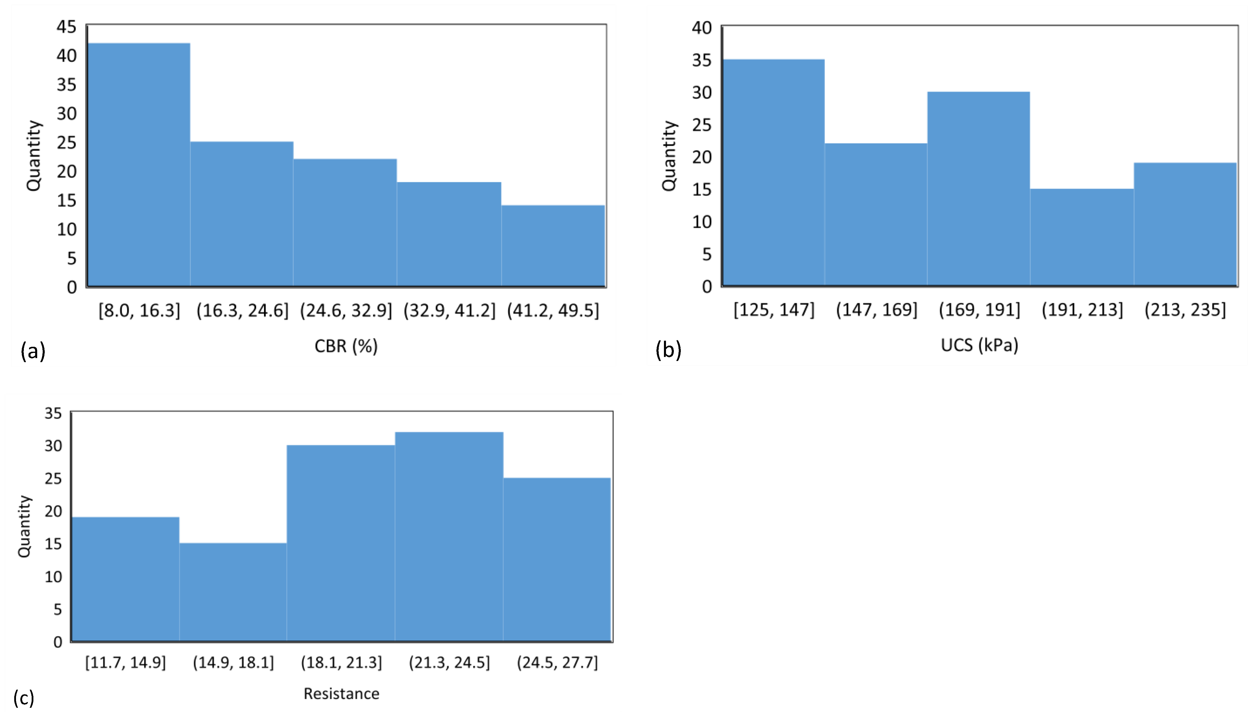
For this study, a dataset consisting of 121 observations was analyzed using a box plot to detect outliers. The process involved computing the median, lower quartile, upper quartile, and interquartile range, followed by calculating the lower and upper fences. Figure 3 indicates that the first quarter parameter of CBR, UCS, and Rvalue values were 14, 141, and 17, respectively, and values of 34, 194, and 24 for the third quarter, respectively. The results demonstrate favorable distribution across the parameter range, from the minimum to the maximum values, with appropriately sized boxes. Additionally, the average parameters within all three boxes fall towards the center of the box, a positive indicator of data dispersion. According to Figure 3, no points were found to exceed the extreme values defined by the computed fences. Furthermore, Figure 4 shows histograms for different outputs.
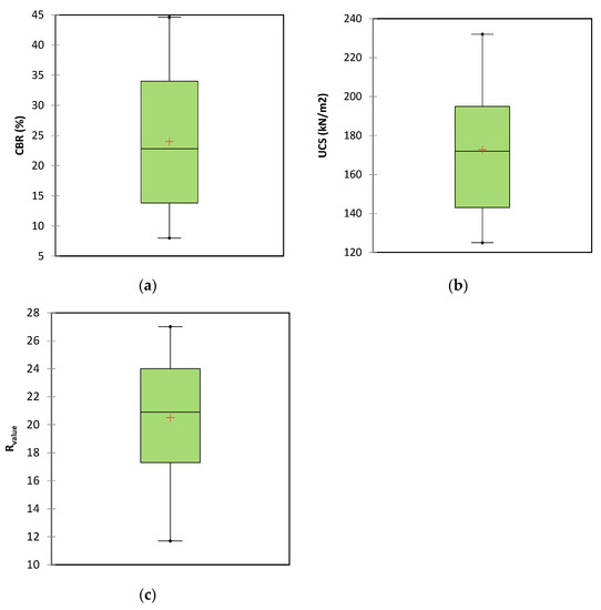
Figure 3.
Box plot of output to find outliers for (a) CBR, (b) UCS, and (c) Rvalue.
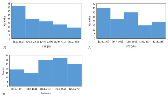
Figure 4.
Histogram plots showing the distribution of (a) CBR, (b) UCS, and (c) Rvalue.
2.2. Testing and Training Databases
The dataset employed in this study was divided into two distinct categories: the training database and the testing database. To achieve this, a random selection process was utilized, assigning 80% of the data to the training database and the remaining 20% to the testing database. The decision to allocate 80% of the data to the training database and the remaining 20% to the testing database is crucial in machine learning due to several reasons. The larger training set allows the model to learn patterns and generalize from the data, while the separate testing set provides an accurate evaluation of the model’s real-world predictive capabilities, avoiding overfitting and ensuring robustness. This division also permits validation, enabling fine-tuning and parameter optimization, resulting in a more realistic assessment of the model’s practical utility, which is essential for guiding decisions on real-world deployment.
Table 2 and Table 3 provide a comprehensive overview of the statistical characteristics, including the minimum, maximum, and average values, for the parameters in the training and testing databases, respectively. The results of the statistical analysis reveal that the two databases share similar characteristics, indicating that the data used for training the artificial intelligence model are representative of the data used for testing the model. This similarity in statistical properties between the training and testing databases is likely to enhance the accuracy and robustness of the developed model. The findings from this study underscore the importance of using representative and well-characterized data for the development of effective and reliable artificial intelligence models. In Table 2 and Table 3, (U95) is 95% Confidence Interval.
Table 2.
Descriptive statistics for the training database.
Table 3.
Descriptive statistics for the testing database.
2.3. Linear Normalizations
In a database context, each input or output variable is linked to specific units of measurement. To mitigate the impact of units and improve the efficiency of artificial intelligence training, a common approach involves data normalization. This process rescales the data to fit within a standardized range, often between zero and one. The normalization is achieved through the application of a linear transformation function, as described below:
The four terms in this equation are Xmax, Xmin, X, and Xnorm, which correspond to maximum, minimum, actual, and normalized values, respectively.
3. Data-Driven Modelling
3.1. Classification and Regression Tree (CART)
In the realm of data mining, decision tree (DT) stands out as a widely used technique known for its simplicity and interpretability [68]. Unlike complex black-box algorithms such as artificial neural networks (ANNs), DT provides a white-box model, making it easier to comprehend and computationally efficient [69]. Among the various types of DT methods, CART (classification and regression trees) has demonstrated a high accuracy and performance for predicting engineering problems [70,71].
A specific type of DT, known as regression tree (RT), employs recursive partitioning to divide the dataset into smaller regions with manageable interactions [70,71]. RT consists of root nodes, interior nodes, branches, and terminal nodes. It utilizes a binary-dividing procedure based on questions about independent variables to achieve optimal splits and construct a tree with high purity [70,71].
To select the best split in RT algorithms, the Gini index is often employed [72]. The partitioning process continues until a stop condition—determined by parameters such as the minimum number of observations, tree depth, or complexity—is met [73]. Pruning can be applied to enhance the tree’s generalization capacity and prevent overfitting [74,75].
An essential capability of CART is its ability to detect and eliminate outliers during the partitioning process [76]. Additionally, CART utilizes principal component analysis (PCA) to identify crucial parameters for modeling [77,78].
Figure 5 shows a typical decision tree, comprising multiple nodes and branches. As depicted in the figure, a combination of nodes and branches forms a leaf. Each node is bifurcated into left and right nodes, guided by specific rules assigned to each branch (for example, if Node A is less than or equal to ‘a’, then proceed to Node C). Ultimately, the final node within each leaf reveals the predicted output (exemplified by nodes D–G in Figure 5).
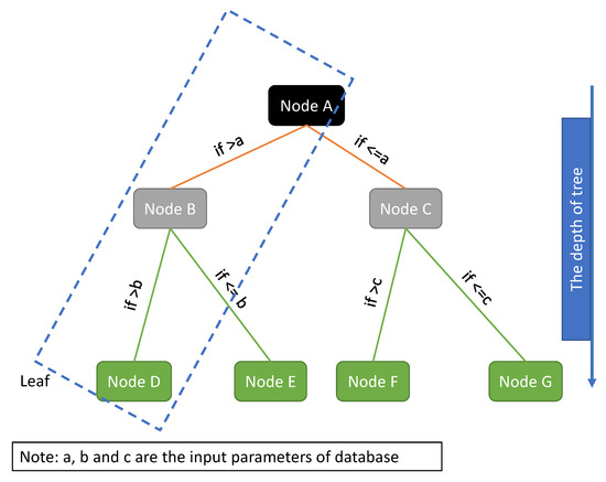
Figure 5.
A typical decision tree for CART.
3.2. Genetic Programming (GP)
Genetic programming (GP) is a remarkable field in artificial intelligence and machine learning, utilizing evolutionary algorithms to create computer programs [79]. Proposed by John Koza in the early 1990s [80], GP has become widely researched and applied across various domains, including image recognition, classification, and prediction. One of its key strengths lies in its flexibility, enabling it to address a diverse range of problems in fields such as engineering, finance, and biology [81]. Moreover, GP’s ability to automatically generate computer programs without human intervention saves valuable time and effort [82]. Additionally, it excels at optimizing complex functions that may be challenging for traditional methods, and its creative nature often leads to unexpected and innovative solutions, potentially uncovering new discoveries.
However, despite its advantages, GP does come with certain drawbacks. Its computational demands can be time consuming, especially when dealing with large search spaces. Furthermore, the generated programs can be challenging to understand and interpret, which can hinder result validation [54,83]. A GP’s performance may also be influenced by the choice of parameters, and it may not always achieve the optimal solution. Additionally, there is a risk of overfitting, as GP-generated programs can become overly specialized to the training data, potentially limiting their generalization to new and unseen data [54,83].
Genetic programming manipulates and optimizes a population of computer models (or programs) to find the best-fitting solution for a given problem. It involves creating an initial population of models, each comprising sets of user-defined functions and terminals. These functions may include mathematical operators (e.g., , , , and /), Boolean logic functions (e.g., AND, OR, and NOT), trigonometric functions (e.g., sin and cos), or other custom functions, while the terminals can consist of numerical constants, logical constants, or variables. These elements are randomly combined in a tree-like structure, forming a computer model that is evolved over generations to improve its performance in solving the problem at hand, as represented in typical GP tree structures. Figure 6 shows an example of a function of .
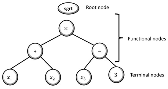
Figure 6.
Common illustration of the tree representation in genetic programming (GP) for the function .
4. Results
In the development of artificial intelligence (AI) systems, the evaluation of various models is of paramount importance. This assessment process relies heavily on statistical parameters, which are instrumental in gauging the performance of AI models. The essential parameters are outlined by Equations (2)–(7), encompassing the mean absolute error (MAE), mean squared error (MSE), root mean squared error (RMSE), mean squared logarithmic error (MSLE), root mean squared logarithmic error (RMSLE), and coefficient of determination (R2). Leveraging these metrics, both researchers and developers can aptly gauge and juxtapose the efficacy of distinct AI models [54].
where N, Xm, and Xp are the number of datasets, actual values, and predicted values, respectively. In addition, and are the averages of the actual and predicted values, respectively. To have the best model, R2 should be 1 and MAE, MSE, RMSE, MSLE, and RMSLE should equal 0.
4.1. Classification and Regression Tree (CART) Results
In this study, the development of the CART model was carried out using the MATLAB 2020 software package. The validity of a CART model hinges on selecting suitable distance ranges and maximum tree depth. Several strategies were tested through trial and error to determine the optimal values for these key parameters. Typically, setting a high value for the maximum tree depth may lead to an excessively complex model. Conversely, opting for a small value for the tree depth may result in the removal of certain input parameters, as the algorithm strives to minimize prediction errors. By iterating through trial and error, the most favorable CART model with well-tuned key parameters can be identified.
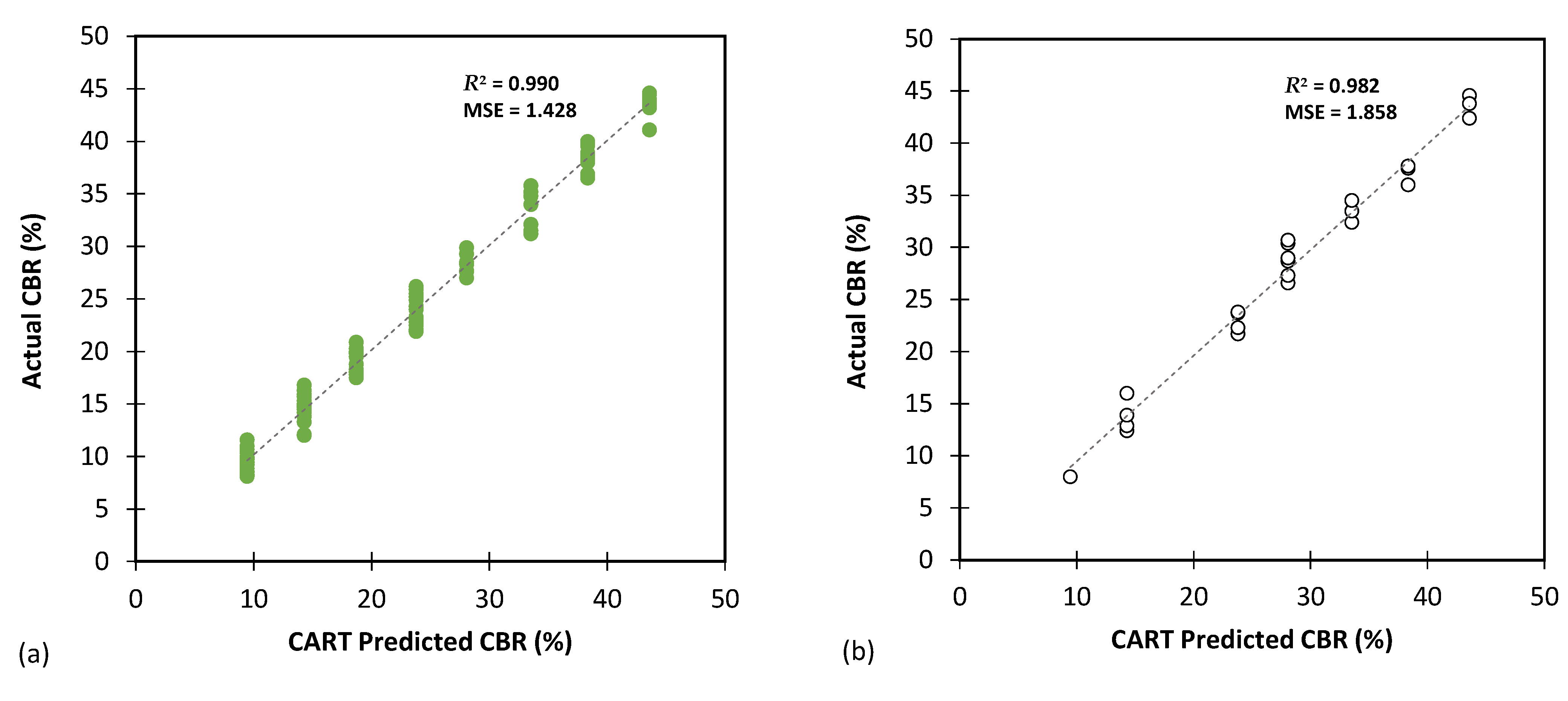
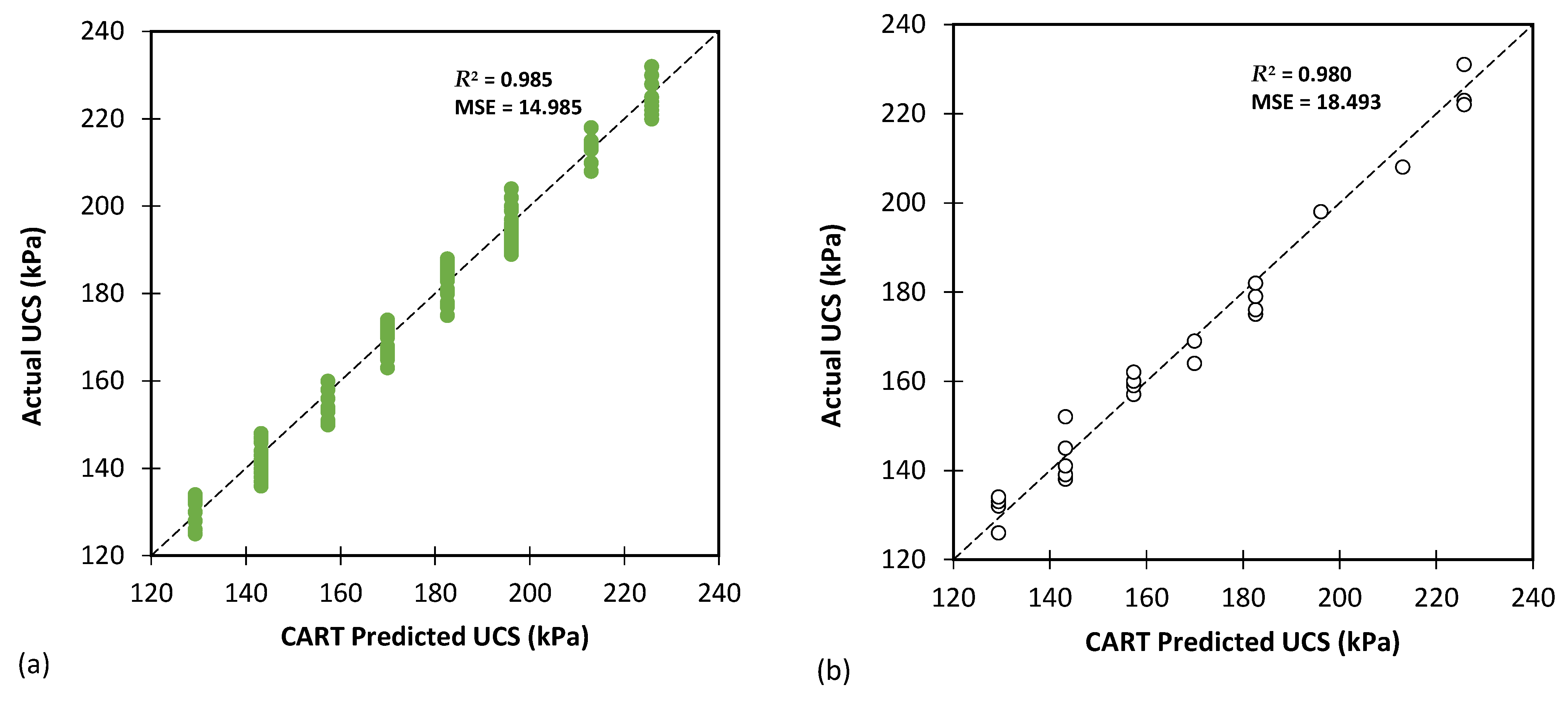
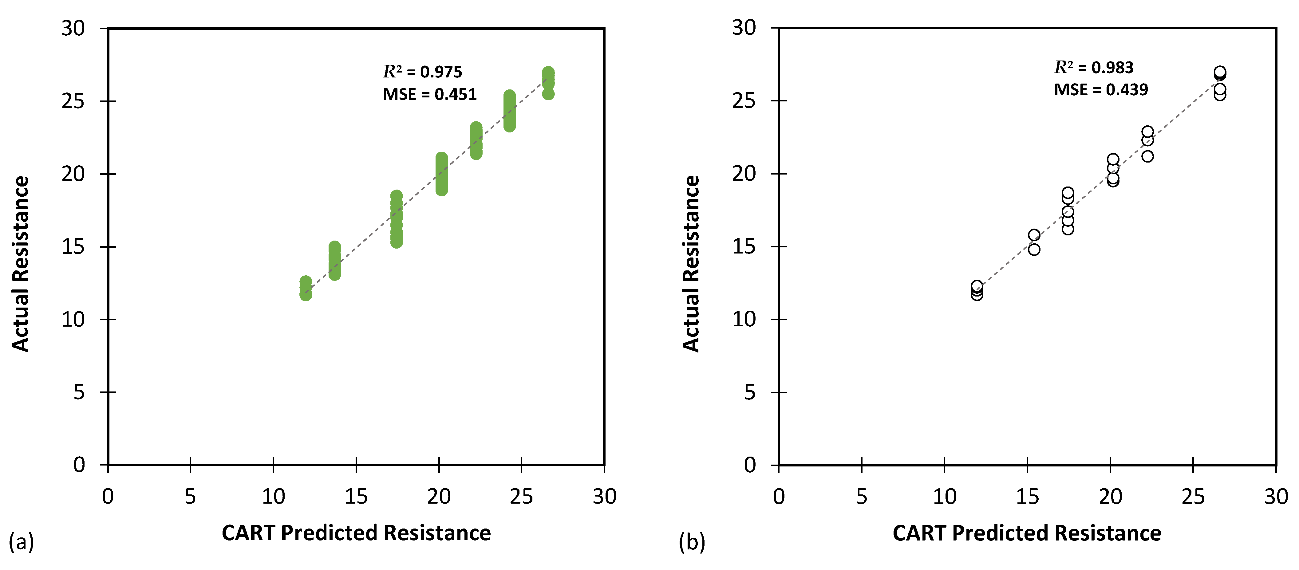
Figure 7, Figure 8 and Figure 9 present the performance of the optimal CART model, showcasing the predicted values versus the actual values obtained from experiments for CBR, UCS, and Rvalue testing, respectively. The results indicate that the CART method demonstrated satisfactory predictive capabilities in accurately determining the CBR, UCS, and Rvalue parameters.
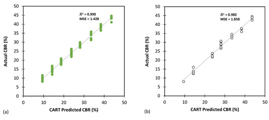
Figure 7.
The results of CART modelling for predicting CBR using (a) training and (b) testing databases.

Figure 8.
The results of CART modelling for predicting UCS using (a) training and (b) testing databases.
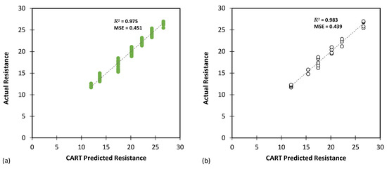
Figure 9.
The results of CART modelling for predicting Rvalue using (a) training and (b) testing databases.
Table 4, Table 5 and Table 6 present a detailed evaluation of the best CART model’s overall performance in predicting the CBR, UCS, and Rvalue parameters. These tables aim to provide comprehensive insights into the accuracy and generalization capabilities of the model on both the training and testing databases. Table 4 focuses on the CART model’s performance in predicting the CBR parameter. The metrics utilized for the evaluation include MAE, MSE, RMSE, MSLE, RMSLE, and R2. The model demonstrates excellent accuracy, with low MAE (0.976 for training and 1.141 for testing) and RMSE (1.195 for training and 1.363 for testing) values. The minimal MSLE and RMSLE values (approximately 0.004) indicate that the model’s predictions were closely aligned with the actual CBR values. Additionally, the high R2 values (0.990 for training and 0.982 for testing) suggest that the model captures a substantial portion of variance in the data, leading to reliable predictions of the CBR parameter.
Table 4.
Overall performance of the best CART model to predict the CBR for both the training and testing databases.
Table 5.
Overall performance of the best CART model to predict the UCS for both the training and testing databases.
Table 6.
Overall performance of the best CART model to predict the resistance value for both the training and testing databases.
Table 5 evaluates the CART model’s performance in predicting the UCS. The model performed admirably with reasonably low MAE (3.262 for training and 3.742 for testing) and RMSE (3.868 for training and 4.300 for testing) values, showcasing its accuracy in predicting the UCS. The MSLE and RMSLE values (both approximately 0.001) further reinforce the strong correlation between predicted and actual values. The high R2 values (0.985 for training and 0.980 for testing) indicate that the model captured a significant portion of variation in the data, resulting in reliable UCS predictions.
Table 6 highlights the CART model’s performance in predicting the Rvalue parameter. Once again, the model delivered impressive results, as indicated by the low MAE (0.539 for training and 0.548 for testing) and RMSE (0.672 for training and 0.663 for testing) values. The MSLE and RMSLE values (both approximately 0.001) reinforce the close correspondence between the predicted and actual values. Moreover, the high R2 values (0.975 for training and 0.983 for testing) demonstrate a strong correlation between the model’s predictions and the actual resistance values.
The consistency in the model’s performance between the training and testing databases across all three tables indicates its ability to generalize unseen data well. Generalization is a critical aspect of machine learning models as it ensures that the model can make accurate predictions on new data, not just the data it was trained on. The fact that the model maintains its accuracy on unseen data suggests that it successfully learned meaningful patterns and relationships from the training database without overfitting. Furthermore, the values of MSLE and RMSLE close to zero in all three tables indicate that the model’s predictions were robust and stable, even for cases where the actual values exhibited significant fluctuations. This property is particularly useful in engineering, where data may have wide variations, and the logarithmic metrics provide a more balanced evaluation of the model’s performance. Moreover, the low values of the MAE, MSE, and RMSE metrics across all three tables indicate that the CART model performed well in minimizing the discrepancy between predicted and actual values. This suggests that the model’s predictions were relatively close to the true values. Small differences between the predicted and actual values are crucial in engineering applications, where precise estimations are vital for design, construction, and safety considerations.
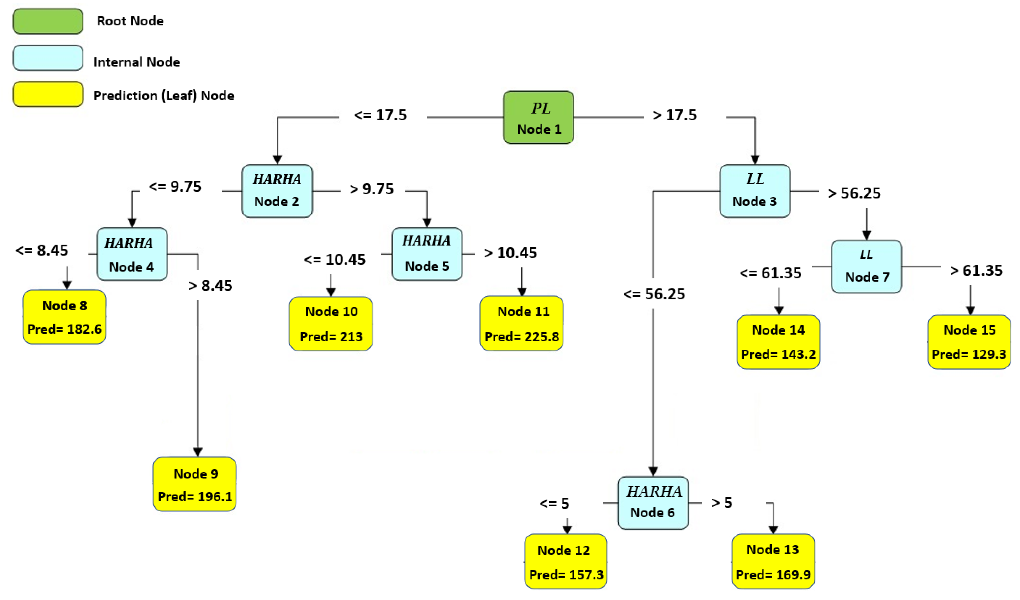
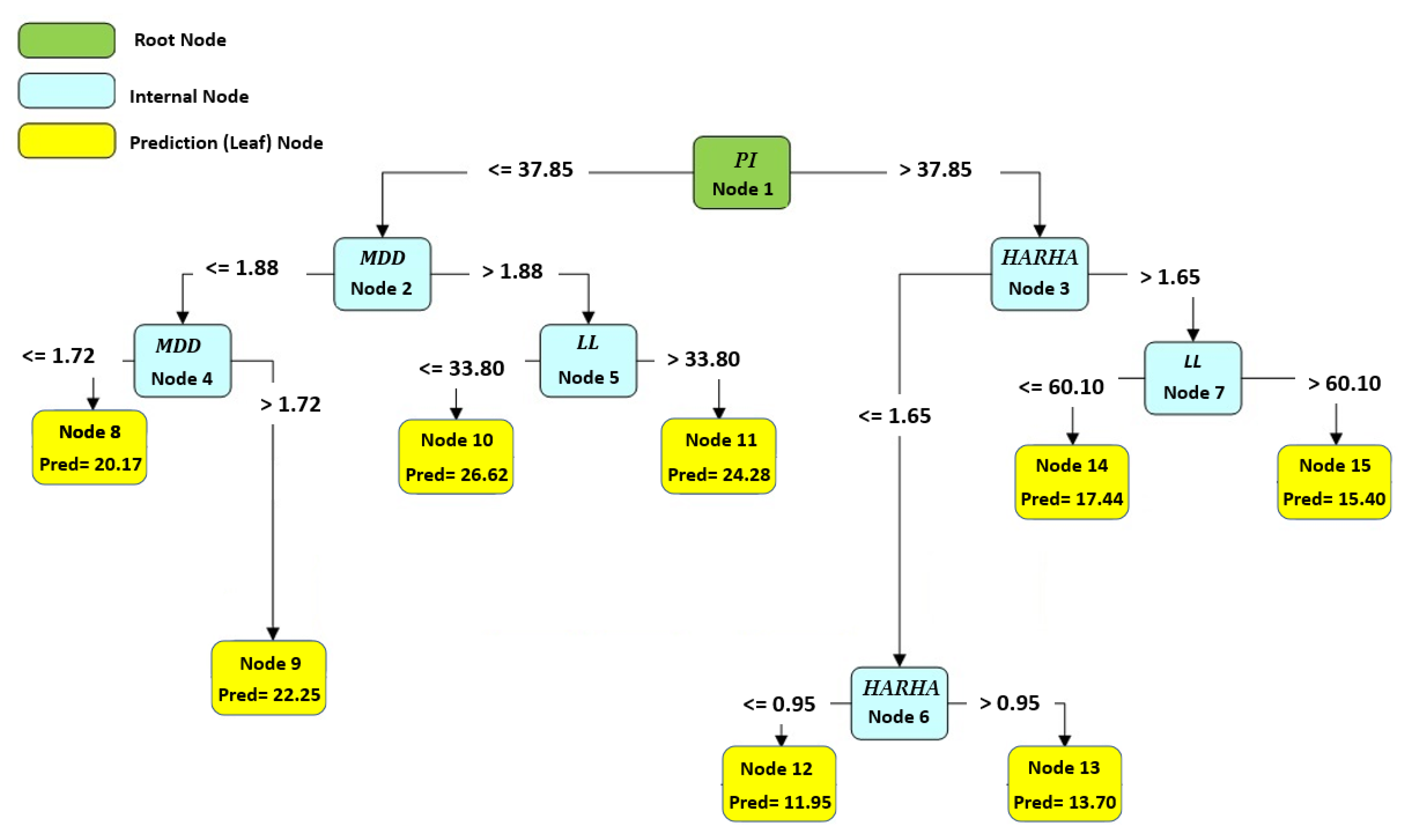
Figure 10, Figure 11 and Figure 12 illustrate the optimal and best CART models for predicting the CBR, UCS, and Rvalue, respectively. Each model consists of 15 nodes, with the LL, PL, and PI serving as the root nodes, respectively. The model determined the number of nodes, which is an outcome of the modeling process. The node count can vary based on the initial tree depth chosen. A higher initial tree depth can result in more nodes, leading to increased model complexity and longer processing times. In this context, an optimal model consisted of 15 nodes.
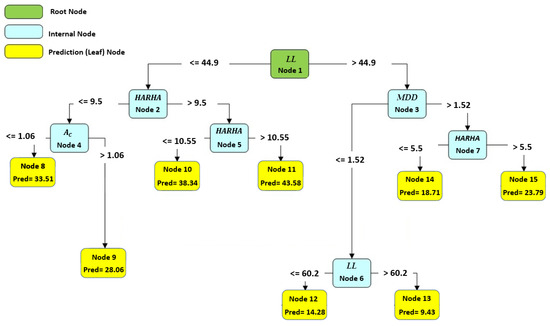
Figure 10.
The best developed CART model to predict the CBR.
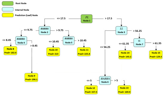
Figure 11.
The best developed CART model to predict the UCS.
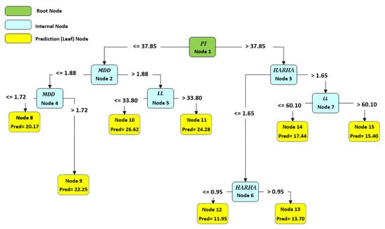
Figure 12.
The best developed CART model to predict the Rvalue.
To obtain the predicted number using any of these models, one must follow the branch rule from node 1 to the end of the tree. These CART models offer valuable tools for engineers and researchers to make accurate predictions based on specific input conditions, facilitating informed decision making in various engineering applications. Further analysis and examination of these models can provide deeper insights into their performance and effectiveness in real-world scenarios.
4.2. Genetic Programming (GP) Results
In this study, the second grey-box model under investigation was genetic programming (GP). To attain the highest performance, several iterations of this model were tested, and the most optimal configuration was identified. Table 7 presents a summary of the crucial parameters used in the GP model, encompassing various properties that were adjusted to achieve the best possible predictive performance for the target variable.
Table 7.
The properties of the optimum GP model for predicting the CBR, UCS, and Rvalue.
The parameters listed in Table 7 were derived from a series of deliberate attempts to refine the model, with the goal of finding the combination of values that produces the best balance of accuracy and performance. This iterative process involves making adjustments, experimenting with different settings, and analyzing the results to reach the most effective configuration. The table serves as a summary of these endeavors, showcasing the parameter values that have been identified as the most optimal based on the criteria of prediction accuracy and overall model quality.
Table 7 provides a detailed summary of the properties of the optimum GP model utilized to predict the CBR, UCS, and Rvalue parameters. Each parameter has its unique configuration in the GP model, which plays a crucial role in determining its predictive performance. The table presents key properties such as the population size, probabilities of GP operations (crossover, mutation, and reproduction), tree structure level, random constants, selection method, tour size, maximum initial and operation tree depth, range for initial values, count of node replacements during crossover, and brood size. By meticulously adjusting these properties for each parameter, the authors aimed to optimize the GP model’s accuracy in providing reliable CBR, UCS, and Rvalue predictions.
For each parameter, the GP model followed the HalfHalf method for generating individuals, leading to linear trees with a depth of 1. The selection method utilized was ‘rank selection’ with a tour size of 2, and various probabilities for GP operations were set, including 0.99 for crossover, 0.99 for mutation, and 0.2 for reproduction. The GP model incorporated two random constants, and it defined the maximum initial and operation tree depth based on values such as 7 for the CBR, 5 for the Rvalue, and 6 for the UCS. The range for initial values varied from 0 to 1, and during crossover, a count of 3 nodes was replaced. Furthermore, the brood size is set at 7 for the CBR, 5 for the Rvalue, and 6 for the UCS. The properties listed in Table 7 offer crucial insights into the GP model’s tailored configuration for predicting the CBR, UCS, and Rvalue.
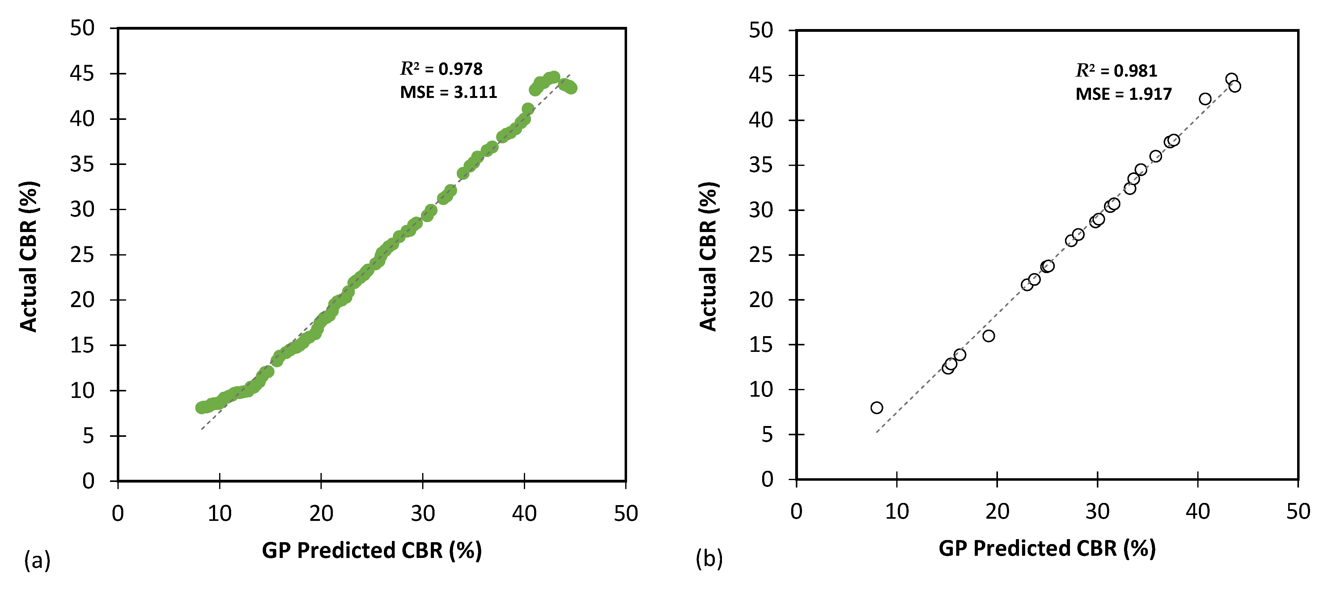
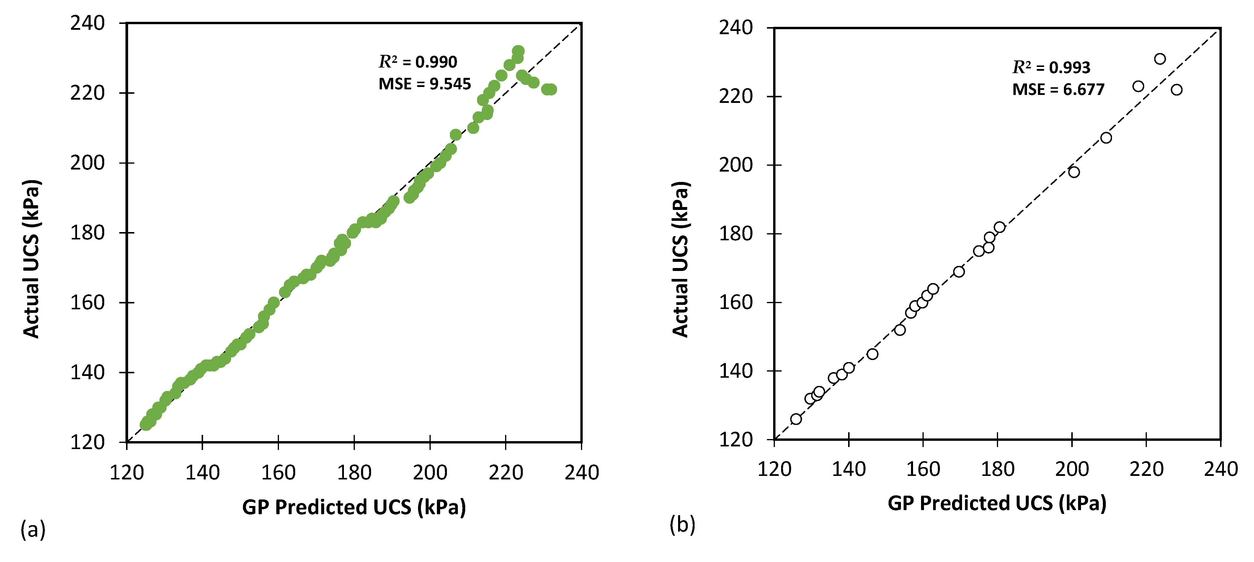
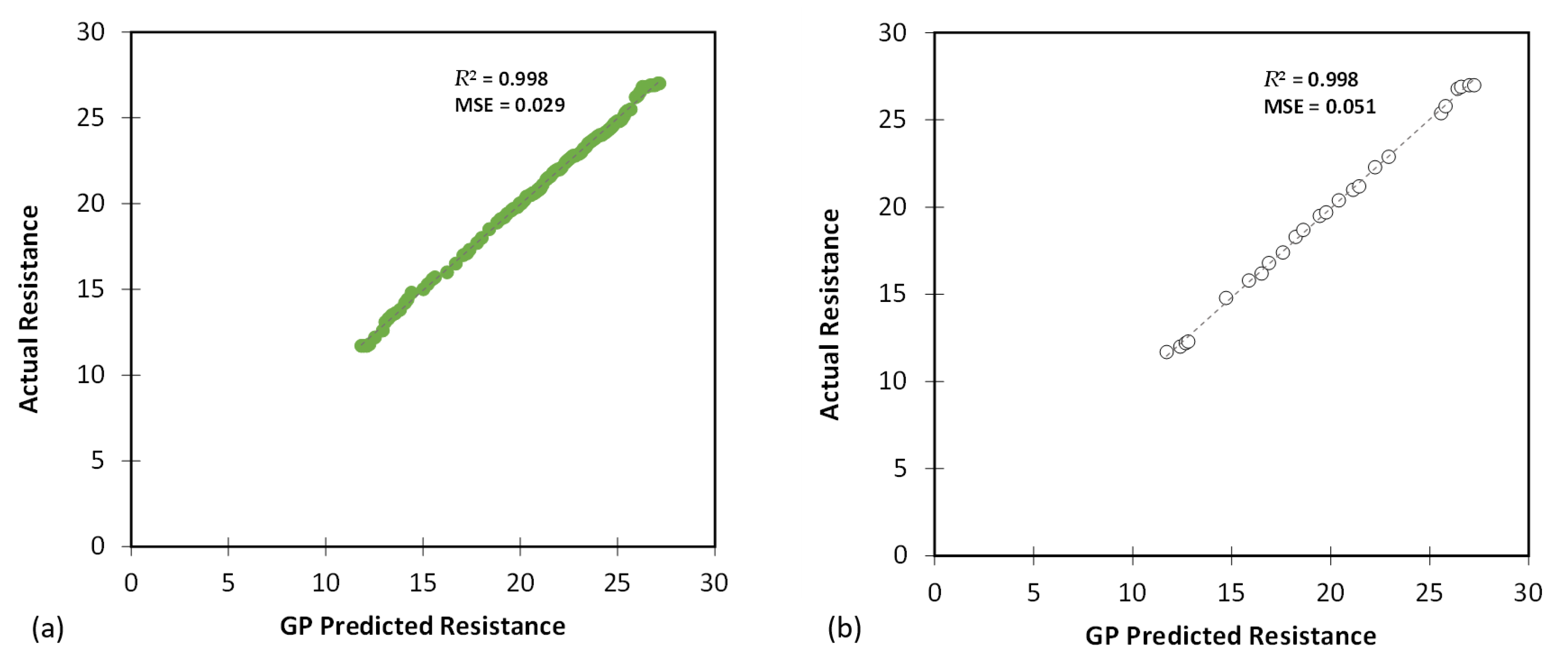
Figure 13, Figure 14 and Figure 15 show comparisons between the predicted CBR, UCS, and Rvalue generated by the GP model and the actual values based on results obtained from the testing and training databases. The GP model exhibited a highly satisfactory performance for predicting the CBR, UCS, and Rvalue parameters.

Figure 13.
The results of GP modelling for predicting the CBR for (a) training and (b) testing databases.
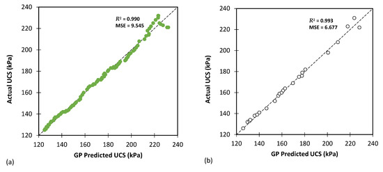
Figure 14.
The results of GP modelling for predicting the UCS for (a) training and (b) testing databases.

Figure 15.
The results of GP modelling for predicting the Rvalue for (a) training and (b) testing databases.
Table 8, Table 9 and Table 10 present the overall performance of the best GP model in predicting the CBR, UCS, and Rvalue parameters for both the training and testing databases, respectively. Each table consists of various metrics that evaluate the model’s predictive capability.
Table 8.
Overall performance of the best GP model to predict the CBR for both the training and testing datasets.
Table 9.
Overall performance of the best GP model to predict the UCS for both the training and testing datasets.
Table 10.
Overall performance of the best GP model to predict the Rvalue for both the training and testing datasets.
Table 8 focuses on predicting the CBR parameters and contains six evaluation metrics, namely MAE, MSE, RMSE, MSLE, RMSLE, and R2. These metrics provide an assessment of the model’s accuracy and goodness of fit. For the training database, MAE was 1.508, indicating an average absolute error of 1.508 between the predicted and actual CBR values. The MAE for the testing dataset was 1.096. Lower MAE and RMSE values are desirable as they indicate a better model performance. The high R2 values (0.978 for training and 0.981 for testing) suggest that the GP model explained a significant portion of the variance in the CBR data.
Table 9 focuses on predicting the UCS and shares the same evaluation metrics as Table 8. The GP model exhibited an impressive performance for predicting the UCS, with lower MAE, MSE, and RMSE values for both the training and testing datasets compared with the CBR predictions reported in Table 8. The R2 values were also higher (0.990 for training and 0.993 for testing), indicating a stronger fit to the UCS data.
Table 10 presents various evaluation metrics associated with the Rvalue predictions. The GP model’s performance for Rvalue predictions was outstanding, with very low MAE, MSE, and RMSE values for both the training and testing datasets. The R2 values were exceptionally high (0.998 for training and 0.998 for testing), demonstrating an excellent fit of the model to the Rvalue data.
Below is the recommended equation obtained from the GP model:
where X1, X2, X3, X4, X5, X6, and X7 are HARHA, LL, PL, PI, wopt, Ac, and MDD, respectively. In addition, the values of R1, R2 and R3 are constants and equal to 0.32, 0.92, and 0.09, respectively.
5. Discussion
5.1. Comparison of CART and GP Models
Table 11, Table 12 and Table 13 provide the results of the proposed CART and GP models in predicting the CBR, UCS, and Rvalue parameters for both the training and testing databases, respectively. The performance metrics evaluated for each model included the MAE, MSE, RMSE, MSLE, RMSLE, and R2.
Table 11.
Results of the proposed CART and GP models in predicting the CBR for both the training and testing databases.
Table 12.
Results of the proposed CART and GP models in predicting the UCS for both the training and testing databases.
Table 13.
Results of the proposed CART and GP models in predicting the Rvalue for both the training and testing databases.
For the CBR predictions (see Table 11), it can be observed that the GP model generally performed slightly worse than CART on the training database across all metrics. However, for the testing database, the performance of the two models was generally on par with each other. For the UCS predictions (see Table 12), the GP model performed better than CART on both the training and testing datasets — that is, the GP model consistently showed lower MAE, MSE, RMSE, MSLE, and RMSLE values compared to those obtained for the CART model. For the Rvalue predictions (see Table 13), the GP model significantly outperformed CART on both the training and testing datasets across all metrics. In this regard, the GP model achieved noticeably lower MAE, MSE, RMSE, MSLE, and RMSLE values compared to the CART model.
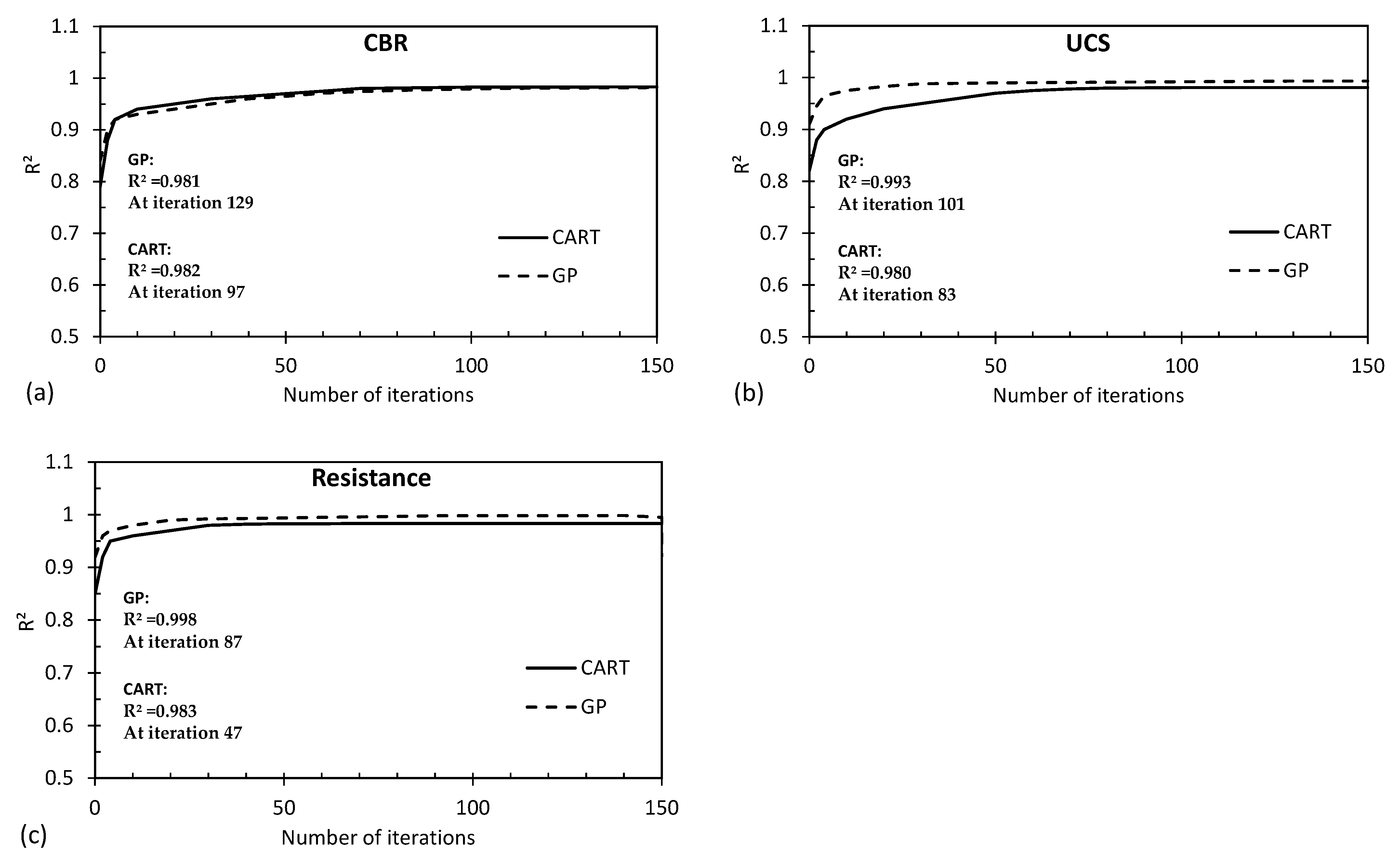
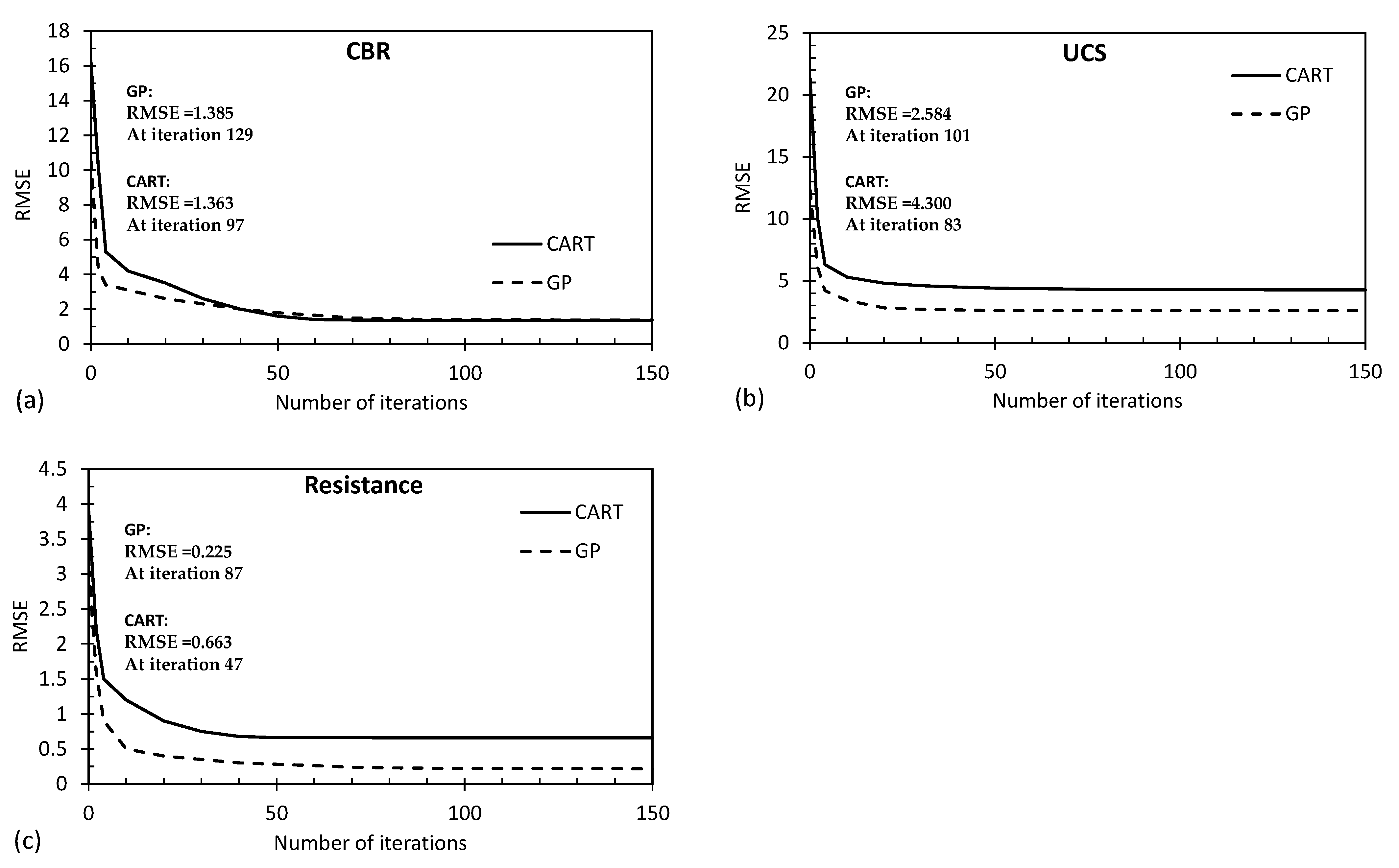
Figure 16 and Figure 17 present convergence curves associated with the output variables (predicted by the proposed CART and GP models) for the R2 and RMSE parameters, respectively. The findings of this study indicate that the GP model initially achieved superior accuracy across all graphs during the first iteration. However, it required a higher number of attempts (iterations) to eventually reach its maximum accuracy level, with the convergence occurring between the 80th and 120th iterations. On the other hand, the CART method exhibited a relatively lower accuracy in the first iteration. However, the CART method demonstrated a quicker ability to enhance its accuracy over successive iterations, enabling it to reach its maximum accuracy level sooner, typically between the 50th and 80th iterations. This suggests that while the GP model initially showed promise in accuracy, the CART method displayed a more efficient improvement trajectory, ultimately reaching its peak accuracy earlier in the iterative process. This insight highlights the dynamic trade-off between initial accuracy and convergence speed between these two modeling approaches.
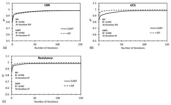
Figure 16.
Convergence curves for the R2 parameter associated with (a) CBR, (b) UCS, and (c) Rvalue predicted by the proposed CART and GP models.
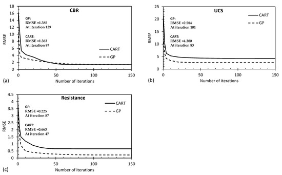
Figure 17.
Convergence curves for the RMSE parameter associated with (a) CBR, (b) UCS, and (c) Rvalue predicted by the proposed CART and GP models.
The difference in accuracy patterns between the GP and CART models can be attributed to the inherent nature of their respective algorithmic structures and optimization processes. The GP model’s initial ‘lucky’ solutions might explain its early higher accuracy, but the CART method’s efficient splitting criteria and incremental refinement process allowed it to quickly catch up and even in some cases surpass the GP model’s accuracy by reaching its peak earlier in the iterative process. The trade-off here is that the CART method’s accuracy improvement curve might have initially started slower, but accelerated as the iterations progressed, leading to faster convergence towards the optimal solution.
5.2. Sensetivity Analysis
In the realm of data-driven modeling, the assessment of input parameters’ significance plays a crucial role. This evaluation involves a systematic process: each individual input parameter is intentionally modified by both increasing and decreasing it by 100%, and then the resulting errors in the models are meticulously observed. This meticulous analysis serves as a tool to gauge the sensitivity of each model to particular parameters. When the error values are higher, it indicates that the model is more sensitive to those specific parameters, whereas lower error values suggest that the parameter being examined has a relatively lesser impact on the overall model performance. This methodology allows us to pinpoint which input parameters significantly influence the model’s outcomes and helps us fine-tune the model for better results.
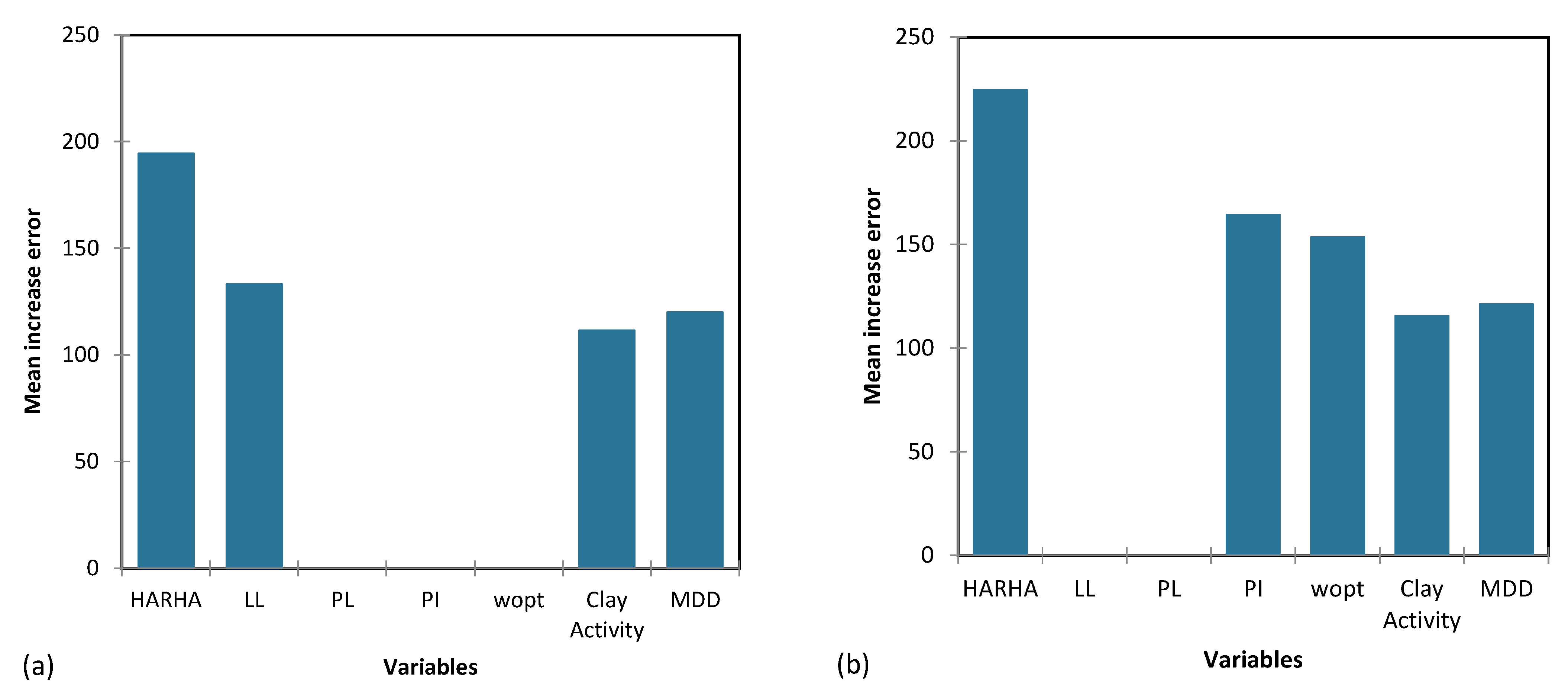
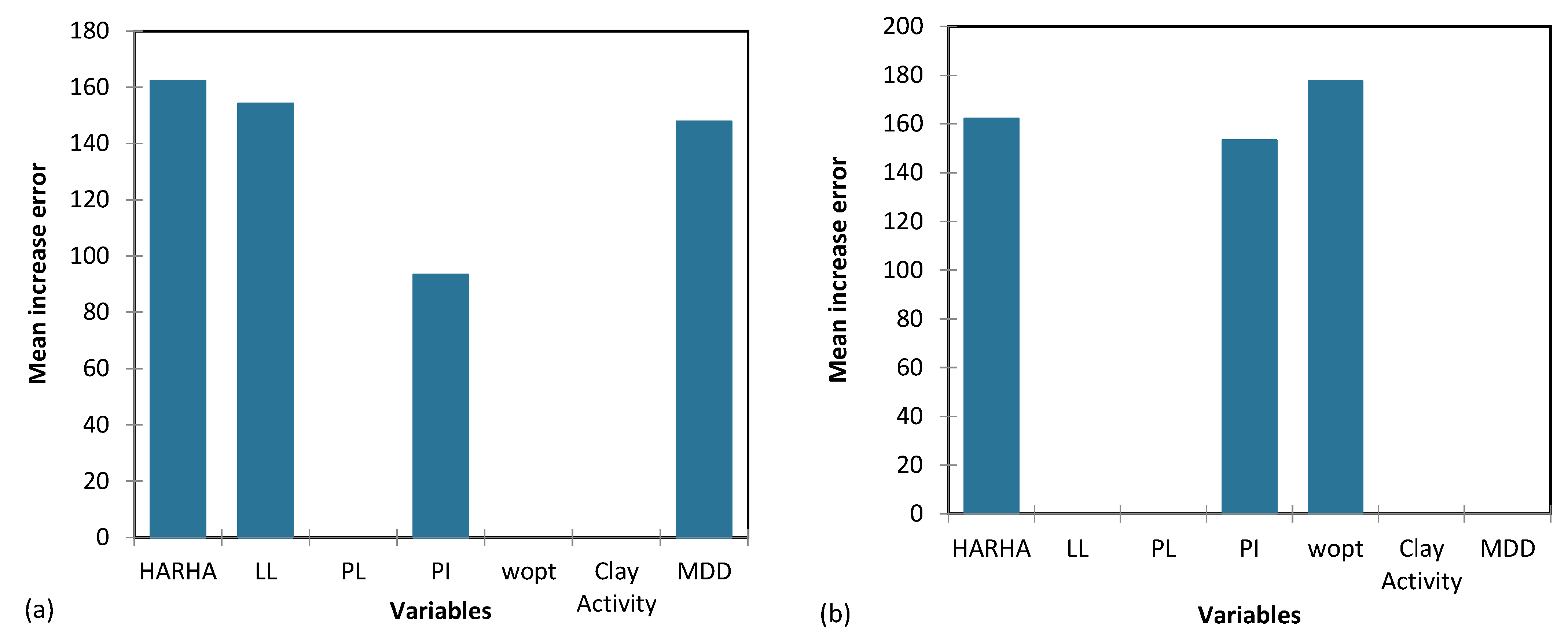
Figure 18, Figure 19 and Figure 20 provide a visual depiction of the importance of the input parameters across the proposed CART and GP models for predicting the CBR, UCS, and Rvalue. These figures offer valuable insights into how the models react to changes in various input parameters and aid in identifying critical factors influencing the predictive performance of the models.

Figure 18.
The importance of input parameters in predicting the CBR for the proposed (a) CART and (b) GP models.
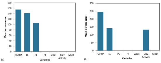
Figure 19.
The importance of input parameters in predicting the UCS for the proposed (a) CART and (b) GP models.
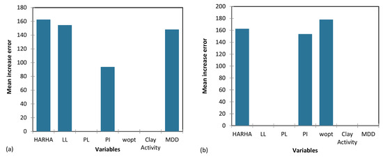
Figure 20.
The importance of input parameters in predicting the Rvalue for the proposed (a) CART and (b) GP models.
Table 14, Table 15 and Table 16 provide a ranking of the input parameters (in terms of their importance) for the proposed models used for predicting the CBR, UCS, and Rvalue, respectively. In this ranking, ‘Rank 1’ corresponds to the highest importance, representing the most critical parameter, while ‘Rank 7’ indicates the lowest importance.
Table 14.
Ranking results of variable importance for the proposed mathematical models to predict CBR.
Table 15.
Ranking results of variable importance for the proposed mathematical models to predict UCS.
Table 16.
Ranking results of variable importance for the proposed mathematical models to predict resistance values.
Based on the results from Table 14, the parameters HARHA, MDD and PI emerge as the most crucial factors for predicting the CBR. In contrast, the parameters PL and clay activity AC hold the least importance in this prediction. Similarly, the findings from Table 15 indicate that the parameters HARHA and LL play pivotal roles, exerting the most influence for UCS predictions. Lastly, as shown in Table 16, the parameters HARHA, LL, and wopt hold the highest levels of importance for predicting the Rvalue. Conversely, parameters PL and AC have the least influence on this prediction.
5.3. Limitations
The present work advances the field by specifically focusing on predicting the soil strength properties for hydrated-lime activated rice husk ash-treated soil. It introduces innovative and readily applicable equations and trees derived from grey-box machine learning models, namely CART and GP. The study’s findings on the superior predictive capabilities of GP equations, particularly for the UCS and Rvalue parameters, is a notable contribution. The integration of interpretable yet flexible machine learning models within geotechnical engineering, as practiced in the present study, highlights its potential to enhance decision-making processes and safety measures in future infrastructure development projects.
The study also identifies some limitations and challenges. One limitation is the reliance on a specific laboratory database, which most likely does not represent all possible scenarios encountered in the field; in other words, the generalization of the proposed models to different conditions and materials could be a concern. Additionally, while the GP approach showed promising results, it has its computational demands and may be challenging to interpret, which could pose limitations in real-world engineering applications. The risk of overfitting in GP-generated programs also needs to be addressed to ensure their generalization to unseen data.
6. Conclusions
This paper focused on developing predictive equations and trees using data-driven approaches for three crucial geotechnical properties of hydrated-lime activated rice husk ash-treated soil, namely the California bearing ratio (CBR), unconfined compressive strength (UCS), and resistance value (i.e., Rvalue from an in-situ cone penetrometer test). Two models, namely classification and regression trees (CART) and genetic programming (GP), were employed to predict these properties based on seven input parameters, consisting of hydrated-lime activated rice husk ash (HARHA) content, liquid limit (LL), plastic limit (PL), plasticity index (PI), optimum moisture content (wOMC), clay activity (AC), and maximum dry density (MDD).
The proposed CART and GP models both displayed commendable predictive aptitude for the CBR, UCS, and Rvalue parameters. The models were evaluated using various performance metrics, including MAE, MSE, RMSE, MSLE, RMSLE, and R2. The performance of the models was consistent across both the training and testing datasets, indicating their ability to generalize unseen data well.
Comparing the two models, CART generally outperformed GP in terms of predicting the UCS and Rvalue, particularly on the testing database. However, for the CBR predictions, CART demonstrated a slightly better performance on the training database, while GP performed slightly better on the testing database. Overall, both models proved effective in predicting the geotechnical properties under investigation. Additionally, the study assessed the importance of individual input parameters in the predictive models. This analysis provided valuable insights into the sensitivity of each model to specific parameters, helping identify critical factors influencing the models’ performance. The findings of this study contribute to the understanding of using data-driven approaches in predicting engineering properties of soils, which can have significant applications in geotechnical engineering and construction. The developed models offer valuable tools for engineers and researchers to make accurate predictions based on specific input conditions, facilitating informed decision making in various geoengineering applications.
Author Contributions
Conceptualization, A.B., K.K. and A.S.; methodology, A.B.; software, A.B. and F.D.; validation, A.B. and K.K.; formal analysis, A.B. and F.D.; investigation, A.B.; resources, A.B. and K.K.; data curation, A.B.; writing—original draft preparation, A.B. and K.K.; writing—review and editing, A.B., A.S. and F.D.; visualization, A.B. and F.D.; supervision, A.B. and A.S.; project administration, A.B. and K.K.; funding acquisition, A.B. All authors have read and agreed to the published version of the manuscript.
Funding
This research received no external funding.
Data Availability Statement
All data generated or analyzed during this study are included in this published article.
Conflicts of Interest
The authors declare no conflict of interest.
References
- Baghbani, A.; Daghistani, F.; Baghbani, H.; Kiany, K.; Bazaz, J.B. Artificial Intelligence-Based Prediction of Geotechnical Impacts of Polyethylene Bottles and Polypropylene on Clayey Soil; EasyChair: Manchester, UK, 2023. [Google Scholar]
- Huang, Y.; Wen, Z. Recent developments of soil improvement methods for seismic liquefaction mitigation. Nat. Hazards 2015, 76, 1927–1938. [Google Scholar] [CrossRef]
- Baghbani, A.; Nguyen, M.D.; Alnedawi, A.; Milne, N.; Baumgartl, T.; Abuel-Naga, H. Improving soil stability with alum sludge: An AI-enabled approach for accurate prediction of California Bearing Ratio. Appl. Sci. 2023, 13, 4934. [Google Scholar] [CrossRef]
- Onyelowe, K.C.; Jalal, F.E.; Onyia, M.E.; Onuoha, I.C.; Alaneme, G.U. Application of gene expression programming to evaluate strength characteristics of hydrated-lime-activated rice husk ash-treated expansive soil. Appl. Comput. Intell. Soft Comput. 2021, 2021, 6686347. [Google Scholar] [CrossRef]
- Dang, L.C.; Fatahi, B.; Khabbaz, H. Behaviour of expansive soils stabilized with hydrated lime and bagasse fibres. Procedia Eng. 2016, 143, 658–665. [Google Scholar] [CrossRef]
- Babu, N.; Poulose, E. Effect of lime on soil properties: A review. Int. Res. J. Eng. Technol. 2018, 5, 606–610. [Google Scholar]
- Chen, R.; Cai, G.; Dong, X.; Pu, S.; Dai, X.; Duan, W. Green utilization of modified biomass by-product rice husk ash: A novel eco-friendly binder for stabilizing waste clay as road material. J. Clean. Prod. 2022, 376, 134303. [Google Scholar] [CrossRef]
- Chandrasekhar, S.A.T.H.Y.; Satyanarayana, K.G.; Pramada, P.N.; Raghavan, P.; Gupta, T.N. Review processing, properties and applications of reactive silica from rice husk—An overview. J. Mater. Sci. 2003, 38, 3159–3168. [Google Scholar] [CrossRef]
- Kumar, A.; Gupta, D. Behavior of cement-stabilized fiber-reinforced pond ash, rice husk ash–soil mixtures. Geotext. Geomembr. 2016, 44, 466–474. [Google Scholar] [CrossRef]
- Hossain, S.S.; Roy, P.K.; Bae, C.J. Utilization of waste rice husk ash for sustainable geopolymer: A review. Constr. Build. Mater. 2021, 310, 125218. [Google Scholar] [CrossRef]
- Khan, R.; Jabbar, A.; Ahmad, I.; Khan, W.; Khan, A.N.; Mirza, J. Reduction in environmental problems using rice-husk ash in concrete. Constr. Build. Mater. 2012, 30, 360–365. [Google Scholar] [CrossRef]
- Meddah, M.S.; Praveenkumar, T.R.; Vijayalakshmi, M.M.; Manigandan, S.; Arunachalam, R. Mechanical and microstructural characterization of rice husk ash and Al2O3 nanoparticles modified cement concrete. Constr. Build. Mater. 2020, 255, 119358. [Google Scholar] [CrossRef]
- Zareei, S.A.; Ameri, F.; Dorostkar, F.; Ahmadi, M. Rice husk ash as a partial replacement of cement in high strength concrete containing micro silica: Evaluating durability and mechanical properties. Case Stud. Constr. Mater. 2017, 7, 73–81. [Google Scholar] [CrossRef]
- Patel, Y.J.; Shah, N. Enhancement of the properties of ground granulated blast furnace slag based self compacting geopolymer concrete by incorporating rice husk ash. Constr. Build. Mater. 2018, 171, 654–662. [Google Scholar] [CrossRef]
- Nalli, B.R.; Vysyaraju, P. March. Utilization of ceramic waste powder and rice husk ash as a partial replacement of cement in concrete. IOP Conf. Ser. Earth Environ. Sci. 2022, 982, 012003. [Google Scholar] [CrossRef]
- Jhatial, A.A.; Goh, W.I.; Mo, K.H.; Sohu, S.; Bhatti, I.A. Green and sustainable concrete–the potential utilization of rice husk ash and egg shells. Civ. Eng. J. 2019, 5, 74–81. [Google Scholar] [CrossRef]
- Baghbani, A.; Daghistani, F.; Kiany, K.; Shalchiyan, M.M. AI-Based Prediction of Strength and Tensile Properties of Expansive Soil Stabilized with Recycled Ash and Natural Fibers; EasyChair: Manchester, UK, 2023. [Google Scholar]
- Jafer, H.M.; Atherton, W.; Sadique, M.; Ruddock, F.; Loffill, E. Development of a new ternary blended cementitious binder produced from waste materials for use in soft soil stabilisation. J. Clean. Prod. 2018, 172, 516–528. [Google Scholar] [CrossRef]
- Sandhu, R.K.; Siddique, R. Influence of rice husk ash (RHA) on the properties of self-compacting concrete: A review. Constr. Build. Mater. 2017, 153, 751–764. [Google Scholar] [CrossRef]
- Diniz, H.A.; dos Anjos, M.A.; Rocha, A.K.; Ferreira, R.L. Effects of the use of agricultural ashes, metakaolin and hydrated-lime on the behavior of self-compacting concretes. Constr. Build. Mater. 2022, 319, 126087. [Google Scholar] [CrossRef]
- Sata, V.; Tangpagasit, J.; Jaturapitakkul, C.; Chindaprasirt, P. Effect of W/B ratios on pozzolanic reaction of biomass ashes in Portland cement matrix. Cem. Concr. Compos. 2012, 34, 94–100. [Google Scholar] [CrossRef]
- Liang, G.; Zhu, H.; Zhang, Z.; Wu, Q.; Du, J. Investigation of the waterproof property of alkali-activated metakaolin geopolymer added with rice husk ash. J. Clean. Prod. 2019, 230, 603–612. [Google Scholar] [CrossRef]
- Hasnain, M.H.; Javed, U.; Ali, A.; Zafar, M.S. Eco-friendly utilization of rice husk ash and bagasse ash blend as partial sand replacement in self-compacting concrete. Constr. Build. Mater. 2021, 273, 121753. [Google Scholar] [CrossRef]
- Afrin, H. A review on different types soil stabilization techniques. Int. J. Transp. Eng. Technol. 2017, 3, 19–24. [Google Scholar] [CrossRef]
- Onyelowe, K.C.; Iqbal, M.; Jalal, F.E.; Onyia, M.E.; Onuoha, I.C. Application of 3-algorithm ANN programming to predict the strength performance of hydrated-lime activated rice husk ash treated soil. Multiscale Multidiscip. Model. Exp. Des. 2021, 4, 259–274. [Google Scholar] [CrossRef]
- Nguyen, M.D.; Baghbani, A.; Alnedawi, A.; Ullah, S.; Kafle, B.; Thomas, M.; Moon, E.M.; Milne, N.A. Investigation on the suitability of aluminium-based water treatment sludge as a sustainable soil replacement for road construction. Transp. Eng. 2023, 12, 100175. [Google Scholar] [CrossRef]
- Jong, S.C.; Ong, D.E.L.; Oh, E. State-of-the-art review of geotechnical-driven artificial intelligence techniques in underground soil-structure interaction. Tunn. Undergr. Space Technol. 2021, 113, 103946. [Google Scholar] [CrossRef]
- Esmaeili-Falak, M.; Benemaran, R.S. Ensemble deep learning-based models to predict the resilient modulus of modified base materials subjected to wet-dry cycles. Geomech. Eng. 2023, 32, 583–600. [Google Scholar]
- Sarkhani Benemaran, R.; Esmaeili-Falak, M.; Javadi, A. Predicting resilient modulus of flexible pavement foundation using extreme gradient boosting based optimised models. Int. J. Pavement Eng. 2022, 12, 1–20. [Google Scholar] [CrossRef]
- Li, D.; Zhang, X.; Kang, Q.; Tavakkol, E. Estimation of unconfined compressive strength of marine clay modified with recycled tiles using hybridized extreme gradient boosting method. Constr. Build. Mater. 2023, 393, 131992. [Google Scholar] [CrossRef]
- Esmaeili-Falak, M.; Katebi, H.; Vadiati, M.; Adamowski, J. Predicting triaxial compressive strength and Young’s modulus of frozen sand using artificial intelligence methods. J. Cold Reg. Eng. 2019, 33, 04019007. [Google Scholar] [CrossRef]
- Liu, X.F.; Zhu, H.H.; Wu, B.; Li, J.; Liu, T.X.; Shi, B. Artificial intelligence-based fiber optic sensing for soil moisture measurement with different cover conditions. Measurement 2023, 206, 112312. [Google Scholar] [CrossRef]
- Nassr, A.; Esmaeili-Falak, M.; Katebi, H.; Javadi, A. A new approach to modeling the behavior of frozen soils. Eng. Geol. 2018, 246, 82–90. [Google Scholar] [CrossRef]
- Lawal, A.I.; Kwon, S. Application of artificial intelligence to rock mechanics: An overview. J. Rock Mech. Geotech. Eng. 2021, 13, 248–266. [Google Scholar] [CrossRef]
- Zhang, Q.; Song, J. The application of machine learning to rock mechanics. In Proceedings of the 7th ISRM Congress, Aachen, Germany, 16–20 September 1991. [Google Scholar]
- Tariq, Z.; Elkatatny, S.M.; Mahmoud, M.A.; Abdulraheem, A.; Abdelwahab, A.Z.; Woldeamanuel, M. Estimation of rock mechanical parameters using artificial intelligence tools. In Proceedings of the ARMA US Rock Mechanics/Geomechanics Symposium ARMA-2017, San Francisco, CA, USA, 25–28 June 2017. [Google Scholar]
- Mei, X.; Li, C.; Sheng, Q.; Cui, Z.; Zhou, J.; Dias, D. Development of a hybrid artificial intelligence model to predict the uniaxial compressive strength of a new aseismic layer made of rubber-sand concrete. Mech. Adv. Mater. Struct. 2023, 30, 2185–2202. [Google Scholar] [CrossRef]
- Khajehzadeh, M.; Taha, M.R.; Keawsawasvong, S.; Mirzaei, H.; Jebeli, M. An effective artificial intelligence approach for slope stability evaluation. IEEE Access 2022, 10, 5660–5671. [Google Scholar] [CrossRef]
- Costa, S.; Kodikara, J.; Barbour, S.L.; Fredlund, D.G. Theoretical analysis of desiccation crack spacing of a thin, long soil layer. Acta Geotech. 2018, 13, 39–49. [Google Scholar] [CrossRef]
- Chen, S.H.; Jakeman, A.J.; Norton, J.P. Artificial intelligence techniques: An introduction to their use for modelling environmental systems. Math. Comput. Simul. 2008, 78, 379–400. [Google Scholar] [CrossRef]
- Daghistani, F.; Baghbani, A.; Abuel Naga, H.; Faradonbeh, R.S. Internal Friction Angle of Cohesionless Binary Mixture Sand–Granular Rubber Using Experimental Study and Machine Learning. Geosciences 2023, 13, 197. [Google Scholar] [CrossRef]
- Baghbani, A.; Costa, S.; Lu, Y.; Soltani, A.; Abuel-Naga, H.; Samui, P. Effects of particle shape on shear modulus of sand using dynamic simple shear testing. Arab. J. Geosci. 2023, 16, 422. [Google Scholar] [CrossRef]
- Baghbani, A.; Costa, S.; Faradonbeh, R.S.; Soltani, A.; Baghbani, H. Modeling the effects of particle shape on damping ratio of dry sand by simple shear testing and artificial intelligence. Appl. Sci. 2023, 13, 4363. [Google Scholar] [CrossRef]
- Baghbani, A.; Abuel-Naga, H.; Shirani Faradonbeh, R.; Costa, S.; Almasoudi, R. Ultrasonic Characterization of Compacted Salty Kaolin–Sand Mixtures Under Nearly Zero Vertical Stress Using Experimental Study and Machine Learning. Geotech. Geol. Eng. 2023, 41, 2987–3012. [Google Scholar] [CrossRef]
- Zhang, X.; Wu, X.; Park, Y.; Zhang, T.; Huang, X.; Xiao, F.; Usmani, A. Perspectives of big experimental database and artificial intelligence in tunnel fire research. Tunn. Undergr. Space Technol. 2021, 108, 103691. [Google Scholar] [CrossRef]
- Ayawah, P.E.; Sebbeh-Newton, S.; Azure, J.W.; Kaba, A.G.; Anani, A.; Bansah, S.; Zabidi, H. A review and case study of Artificial intelligence and Machine learning methods used for ground condition prediction ahead of tunnel boring Machines. Tunn. Undergr. Space Technol. 2022, 125, 104497. [Google Scholar] [CrossRef]
- Lai, J.; Qiu, J.; Feng, Z.; Chen, J.; Fan, H. Prediction of soil deformation in tunnelling using artificial neural networks. Comput. Intell. Neurosci. 2016, 33. [Google Scholar] [CrossRef]
- Allawi, M.F.; Jaafar, O.; Mohamad Hamzah, F.; Abdullah, S.M.S.; El-Shafie, A. Review on applications of artificial intelligence methods for dam and reservoir-hydro-environment models. Environ. Sci. Pollut. Res. 2018, 25, 13446–13469. [Google Scholar] [CrossRef] [PubMed]
- Gomes, M.G.; da Silva, V.H.C.; Pinto, L.F.R.; Centoamore, P.; Digiesi, S.; Facchini, F.; Neto, G.C.D.O. Economic, environmental and social gains of the implementation of artificial intelligence at dam operations toward Industry 4.0 principles. Sustainability 2020, 12, 3604. [Google Scholar] [CrossRef]
- Assaad, R.; El-adaway, I.H. Evaluation and prediction of the hazard potential level of dam infrastructures using computational artificial intelligence algorithms. J. Manag. Eng. 2020, 36, 04020051. [Google Scholar] [CrossRef]
- Johari, A.; Habibagahi, G.; Ghahramani, A. Prediction of SWCC using artificial intelligent systems: A comparative study. Sci. Iran. 2021, 18, 1002–1008. [Google Scholar] [CrossRef]
- Zhang, J.Z.; Phoon, K.K.; Zhang, D.M.; Huang, H.W.; Tang, C. Novel approach to estimate vertical scale of fluctuation based on CPT data using convolutional neural networks. Eng. Geol. 2021, 294, 106342. [Google Scholar] [CrossRef]
- Cao, Z.; Wang, Y. Bayesian model comparison and selection of spatial correlation functions for soil parameters. Struct. Saf. 2014, 49, 10–17. [Google Scholar] [CrossRef]
- Li, K.Q.; Liu, Y.; Kang, Q. Estimating the thermal conductivity of soils using six machine learning algorithms. Int. Commun. Heat Mass Transf. 2022, 136, 106139. [Google Scholar] [CrossRef]
- Pintelas, E.; Livieris, I.E.; Pintelas, P. A grey-box ensemble model exploiting black-box accuracy and white-box intrinsic interpretability. Algorithms 2020, 13, 17. [Google Scholar] [CrossRef]
- Adilkhanova, I.; Ngarambe, J.; Yun, G.Y. Recent advances in black box and white-box models for urban heat island prediction: Implications of fusing the two methods. Renew. Sustain. Energy Rev. 2020, 165, 112520. [Google Scholar] [CrossRef]
- Rodvold, D.M.; McLeod, D.G.; Brandt, J.M.; Snow, P.B.; Murphy, G.P. Introduction to artificial neural networks for physicians: Taking the lid off the black box. Prostate 2001, 46, 39–44. [Google Scholar] [CrossRef]
- Zhang, Q.; Barri, K.; Jiao, P.; Salehi, H.; Alavi, A.H. Genetic programming in civil engineering: Advent, applications and future trends. Artif. Intell. Rev. 2021, 54, 1863–1885. [Google Scholar] [CrossRef]
- Giustolisi, O.; Doglioni, A.; Savic, D.A.; Webb, B.W. A multi-model approach to analysis of environmental phenomena. Environ. Model. Softw. 2007, 22, 674–682. [Google Scholar] [CrossRef]
- Grubbs, F.E. Procedures for detecting outlying observations in samples. Technometrics 1969, 11, 1–21. [Google Scholar] [CrossRef]
- Subramaniam, S.; Palpanas, T.; Papadopoulos, D.; Kalogeraki, V.; Gunopulos, D. Online outlier detection in sensor data using non-parametric models. In Proceedings of the 32nd International Conference on Very Large Data Bases, Seoul, Repulic of Korea, 12–15 September 2006; pp. 187–198. [Google Scholar]
- Yu, G.; Zou, C.; Wang, Z. Outlier detection in functional observations with applications to profile monitoring. Technometrics 2012, 54, 308–318. [Google Scholar] [CrossRef]
- Loureiro, D.; Amado, C.; Martins, A.; Vitorino, D.; Mamade, A.; Coelho, S.T. Water distribution systems flow monitoring and anomalous event detection: A practical approach. Urban Water J. 2016, 13, 242–252. [Google Scholar] [CrossRef]
- Shaukat, K.; Alam, T.M.; Luo, S.; Shabbir, S.; Hameed, I.A.; Li, J.; Abbas, S.K.; Javed, U. A review of time-series anomaly detection techniques: A step to future perspectives. In Advances in Information and Communication: Proceedings of the 2021 Future of Information and Communication Conference (FICC), Vancouver, BC, Canada, 29–30 April 2021; Springer International Publishing: New York, NY, USA, 2022; Volume 1, pp. 865–877. [Google Scholar]
- Marmolejo-Ramos, F.; Tian, T.S. The shifting boxplot. A boxplot based on essential summary statistics around the mean. Int. J. Psychol. Res. 2010, 3, 37–45. [Google Scholar]
- Dawson, R. How significant is a boxplot outlier? J. Stat. Educ. 2011, 19. [Google Scholar] [CrossRef]
- Walker, M.L.; Dovoedo, Y.H.; Chakraborti, S.; Hilton, C.W. An improved boxplot for univariate data. Am. Stat. 2018, 72, 348–353. [Google Scholar] [CrossRef]
- Telikani, A.; Tahmassebi, A.; Banzhaf, W.; Gandomi, A.H. Evolutionary machine learning: A survey. ACM Comput. Surv. (CSUR) 2021, 54, 1–35. [Google Scholar] [CrossRef]
- Alwarthan, S.A.; Aslam, N.; Khan, I.U. Predicting Student Academic Performance at Higher Education Using Data Mining: A Systematic Review. Appl. Comput. Intell. Soft Comput. 2022. [CrossRef]
- Salimi, A.; Faradonbeh, R.S.; Monjezi, M.; Moormann, C. TBM performance estimation using a classification and regression tree (CART) technique. Bull. Eng. Geol. Environ. 2018, 77, 429–440. [Google Scholar] [CrossRef]
- Ren, Q.; Ding, L.; Dai, X.; Jiang, Z.; De Schutter, G. Prediction of compressive strength of concrete with manufactured sand by ensemble classification and regression tree method. J. Mater. Civ. Eng. 2021, 33, 04021135. [Google Scholar] [CrossRef]
- Tangirala, S. Evaluating the impact of GINI index and information gain on classification using decision tree classifier algorithm. Int. J. Adv. Comput. Sci. Appl. 2020, 11, 612–619. [Google Scholar] [CrossRef]
- Kotsiantis, S.B. Decision trees: A recent overview. Artif. Intell. Rev. 2013, 39, 261–283. [Google Scholar] [CrossRef]
- Sun, J.; Hui, X.F. An application of decision tree and genetic algorithms for financial ratios’ dynamic selection and financial distress prediction. In Proceedings of the 2006 International Conference on Machine Learning and Cybernetics, Dalian, China, 13–16 August 2006; pp. 2413–2418. [Google Scholar]
- Wang, T.; Qin, Z.; Jin, Z.; Zhang, S. Handling over-fitting in test cost-sensitive decision tree learning by feature selection, smoothing and pruning. J. Syst. Softw. 2010, 83, 1137–1147. [Google Scholar] [CrossRef]
- Deconinck, E.; Hancock, T.; Coomans, D.; Massart, D.L.; Vander Heyden, Y. Classification of drugs in absorption classes using the classification and regression trees (CART) methodology. J. Pharm. Biomed. Anal. 2005, 39, 91–103. [Google Scholar] [CrossRef] [PubMed]
- Li, X.; Yeh, A.G.O. Urban simulation using principal components analysis and cellular automata for land-use planning. Photogramm. Eng. Remote Sens. 2002, 68, 341–352. [Google Scholar]
- Kheirkhah, A.; Azadeh, A.; Saberi, M.; Azaron, A.; Shakouri, H. Improved estimation of electricity demand function by using of artificial neural network, principal component analysis and data envelopment analysis. Comput. Ind. Eng. 2013, 64, 425–441. [Google Scholar] [CrossRef]
- Kinnear, K.E.; Angeline, P.J.; Spector, L. (Eds.) Advances in Genetic Programming; MIT Press: Cambridge, MA, USA, 1994; Volume 3. [Google Scholar]
- Koza, J.R. Genetic Programming: A Paradigm for Genetically Breeding Populations of Computer Programs to Solve Problems; Stanford University, Department of Computer Science: Stanford, CA, USA, 1994; Volume 34. [Google Scholar]
- Zhong, R.Y.; Newman, S.T.; Huang, G.Q.; Lan, S. Big Data for supply chain management in the service and manufacturing sectors: Challenges, opportunities, and future perspectives. Comput. Ind. Eng. 2016, 101, 572–591. [Google Scholar] [CrossRef]
- Squillero, G. Microgp—An evolutionary assembly program generator. Genet. Program. Evolvable Mach. 2005, 6, 247–263. [Google Scholar] [CrossRef]
- Nguyen, A.T.; Reiter, S.; Rigo, P. A review on simulation-based optimization methods applied to building performance analysis. Appl. Energy 2014, 113, 1043–1058. [Google Scholar] [CrossRef]


Disclaimer/Publisher’s Note: The statements, opinions and data contained in all publications are solely those of the individual author(s) and contributor(s) and not of MDPI and/or the editor(s). MDPI and/or the editor(s) disclaim responsibility for any injury to people or property resulting from any ideas, methods, instructions or products referred to in the content. |
© 2023 by the authors. Licensee MDPI, Basel, Switzerland. This article is an open access article distributed under the terms and conditions of the Creative Commons Attribution (CC BY) license (https://creativecommons.org/licenses/by/4.0/).