
Novel Methods for the Computation of Small-Strain Damping Ratios of Soils from Cyclic Torsional Shear and Free-Vibration Decay Testing


Abstract
:1. Introduction
2. The Proposed Method for Computing the Small-Strain Hysteretic Damping Ratio, λmin, of Soils from Cyclic Torsional Shear Testing
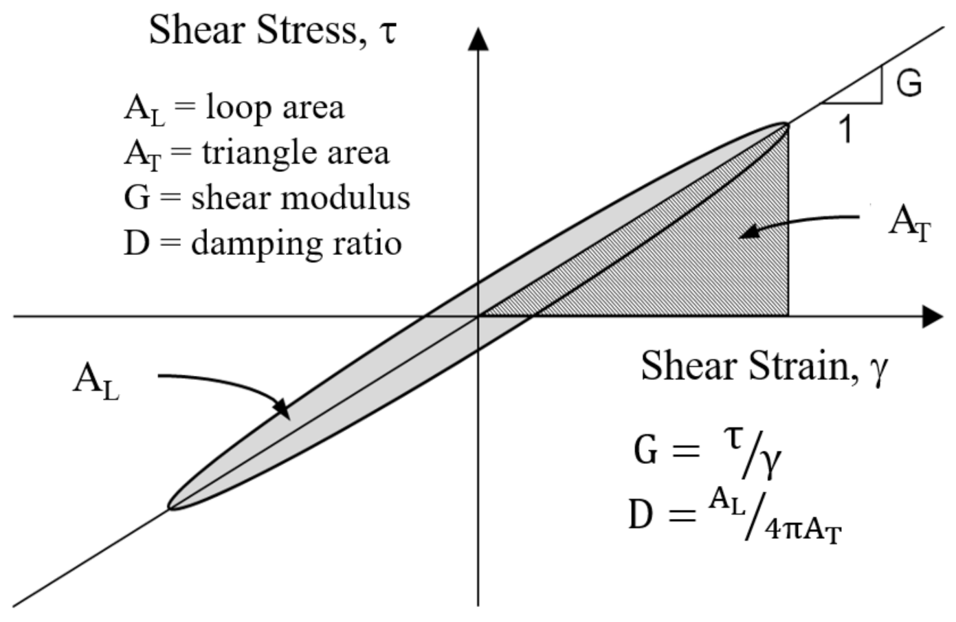
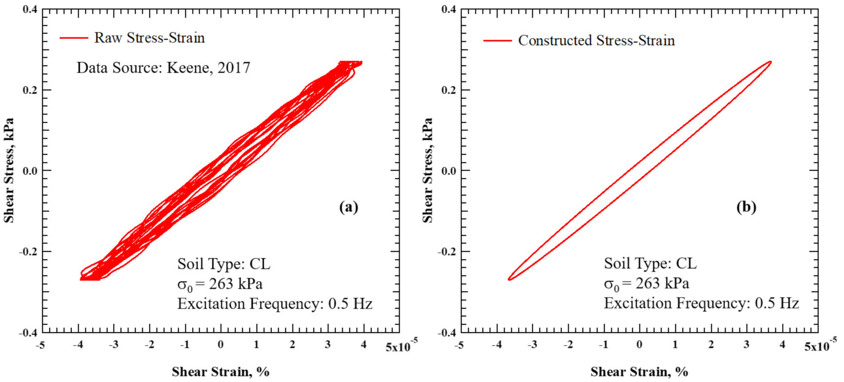
2.1. Conventional Method of λmin Computation from Cyclic Torsional Shear Testing
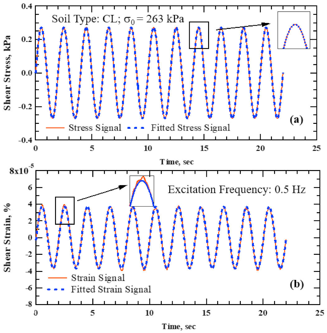
2.2. Proposed Method of λmin Calculated from Torsional Shear Testing
2.2.1. Step I: Phase-Based Method of λmin Computation from TS Testing
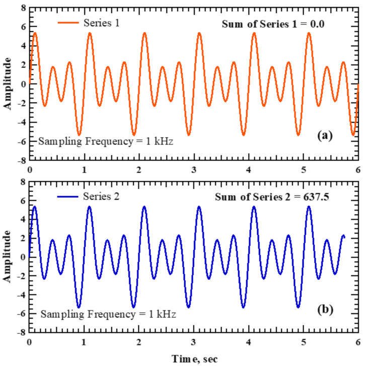
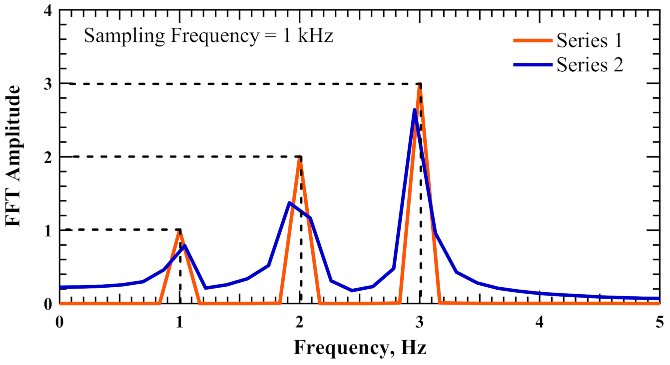
2.2.2. Step II: Fourier Transform Analysis of λmin from TS Testing
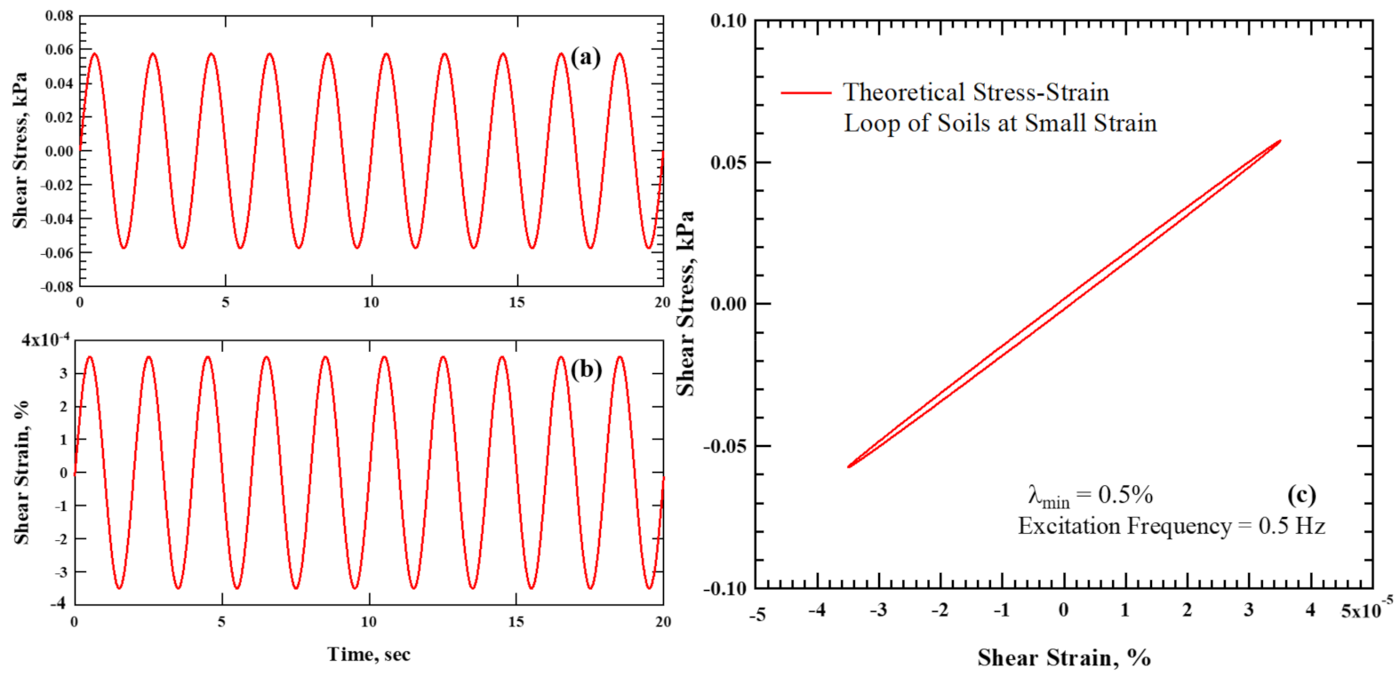
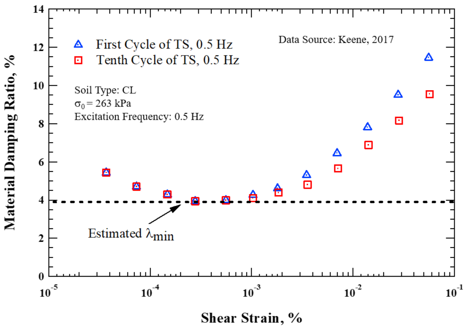
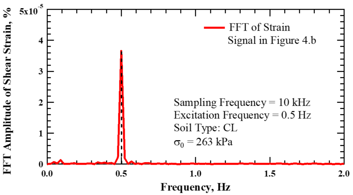
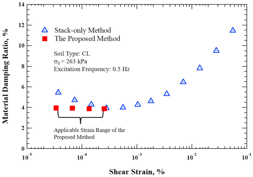
2.3. Application of the Proposed Method to Small-Strain Torsional Shear Testing
3. Computation of the Small-Strain Viscous Damping Ratio, Dmin, Based on the Hilbert Transform
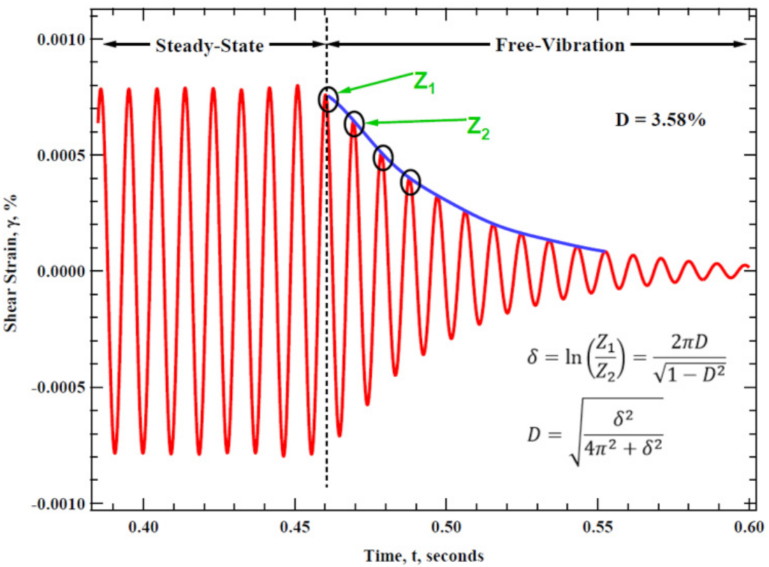
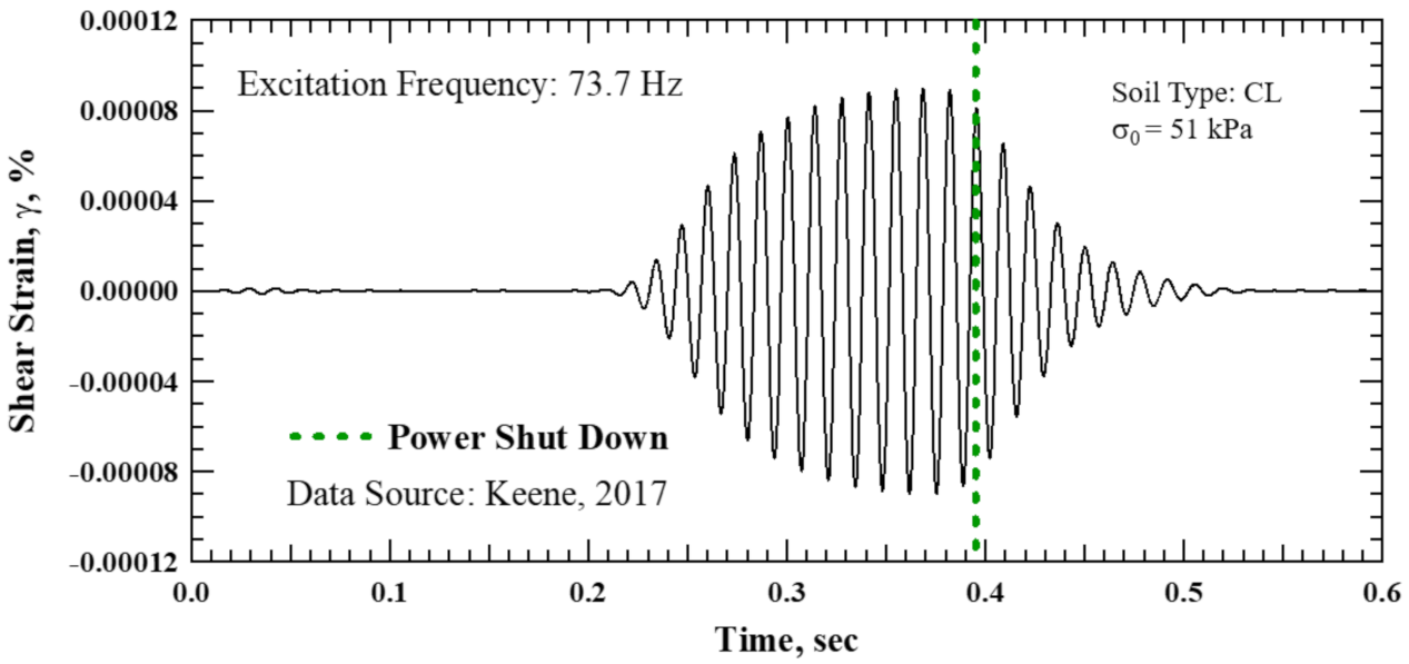
3.1. Conventional Method of Free-Vibration Decay
3.2. Proposed Method for Analyzing FVD
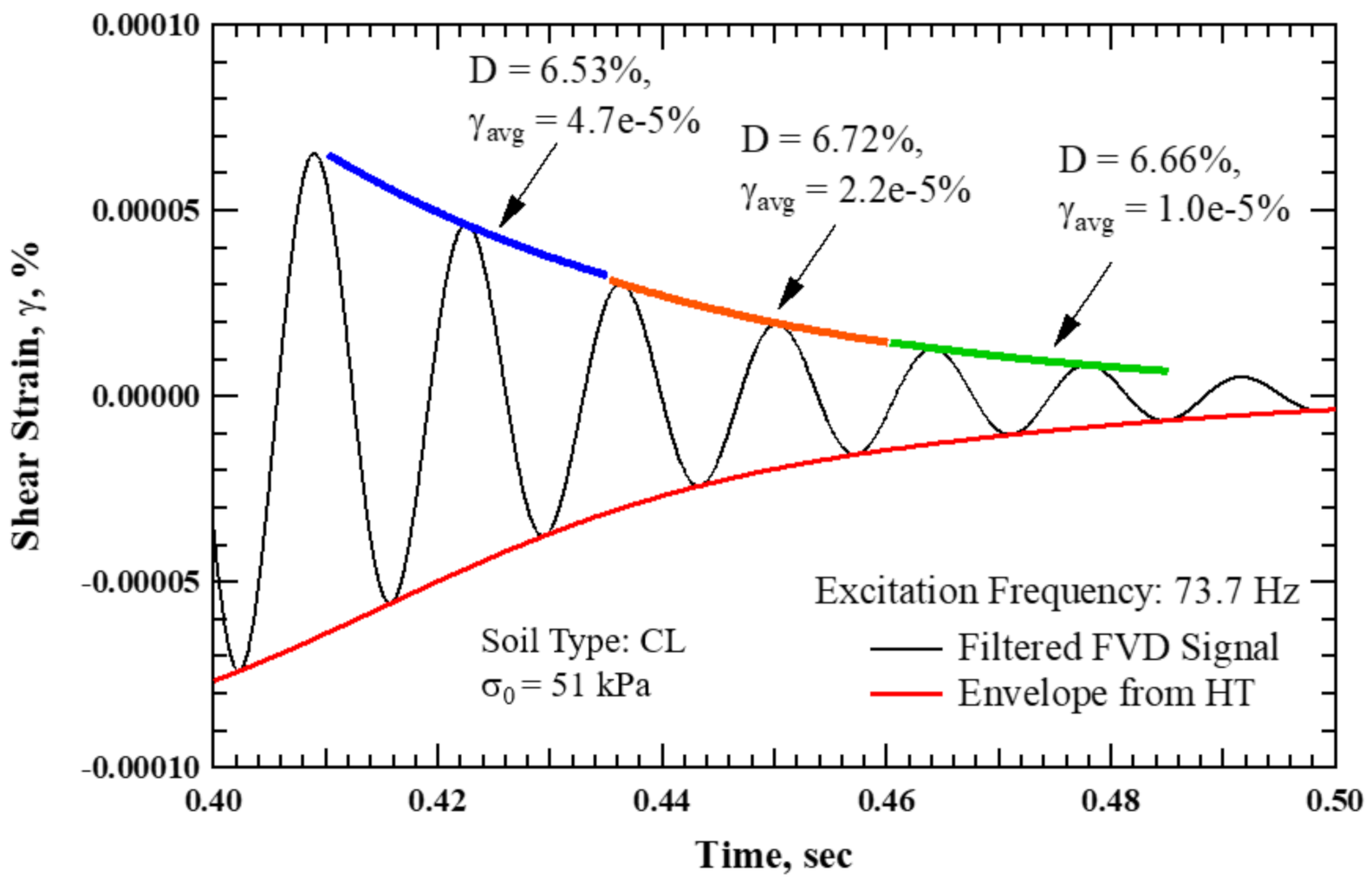
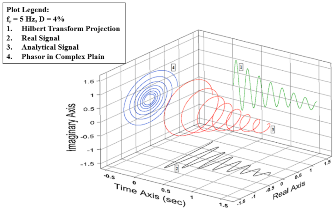
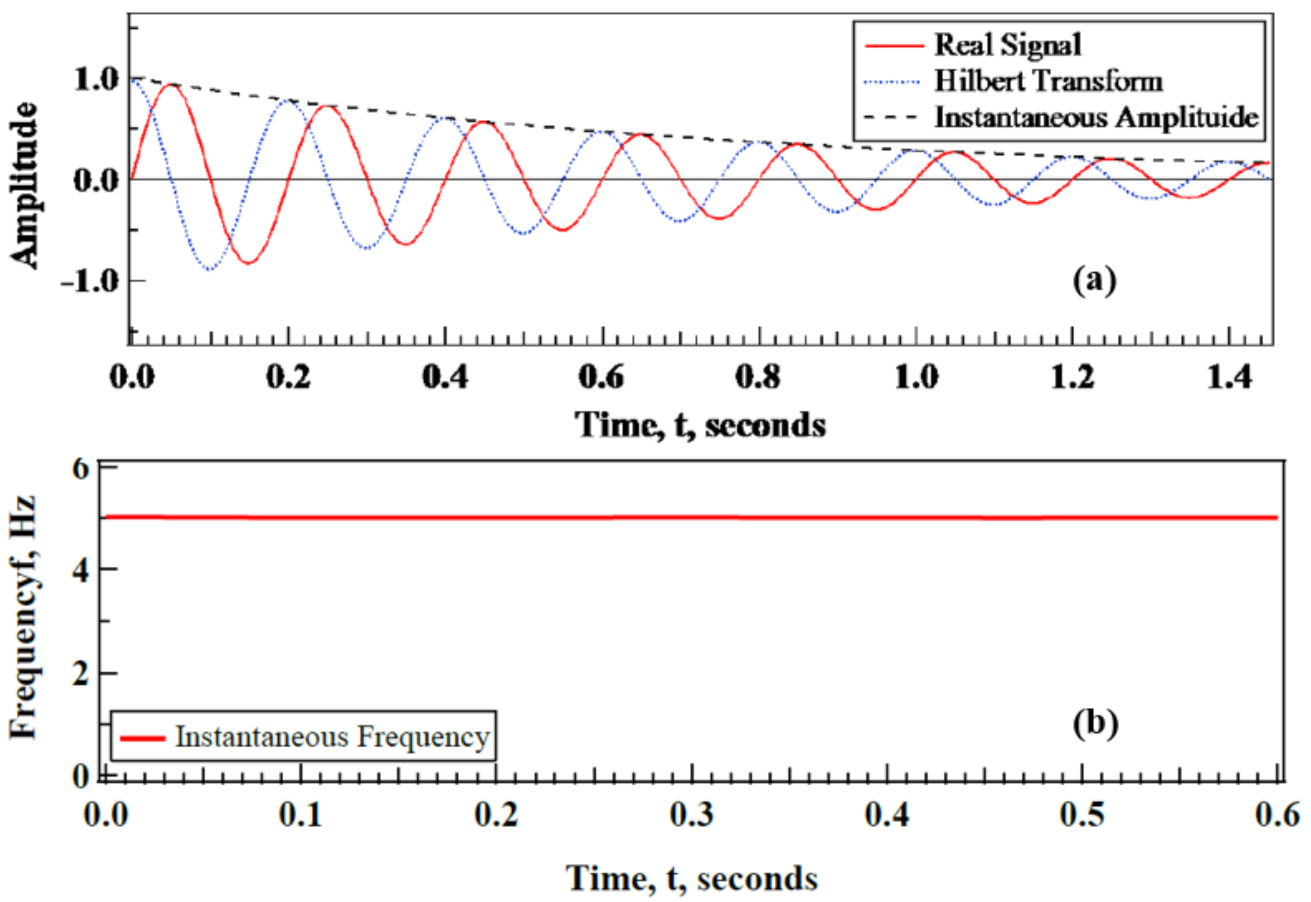
3.2.1. The Hilbert Transform
3.2.2. Conversion of the Instantaneous Amplitude of FVD to the Viscous Damping Ratio
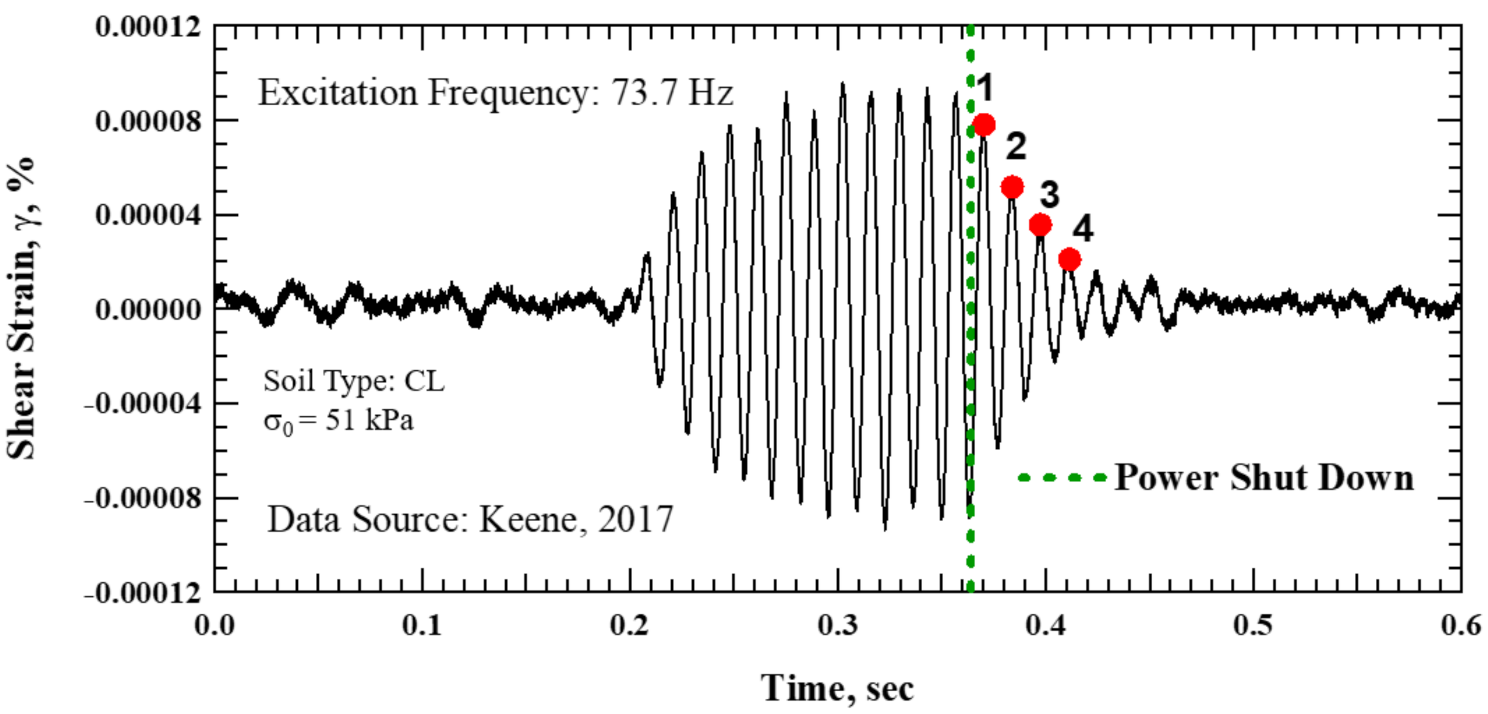
3.3. Application of the Proposed Method in the Analysis of Dmin
3.3.1. Step I: Butterworth Bandpass Filter
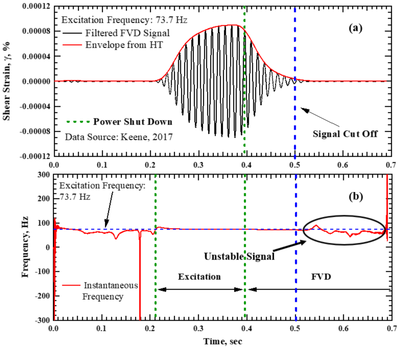
3.3.2. Step II: The Hilbert Transform and Signal Truncation
3.3.3. Step III: Data Fitting and Damping Calculation
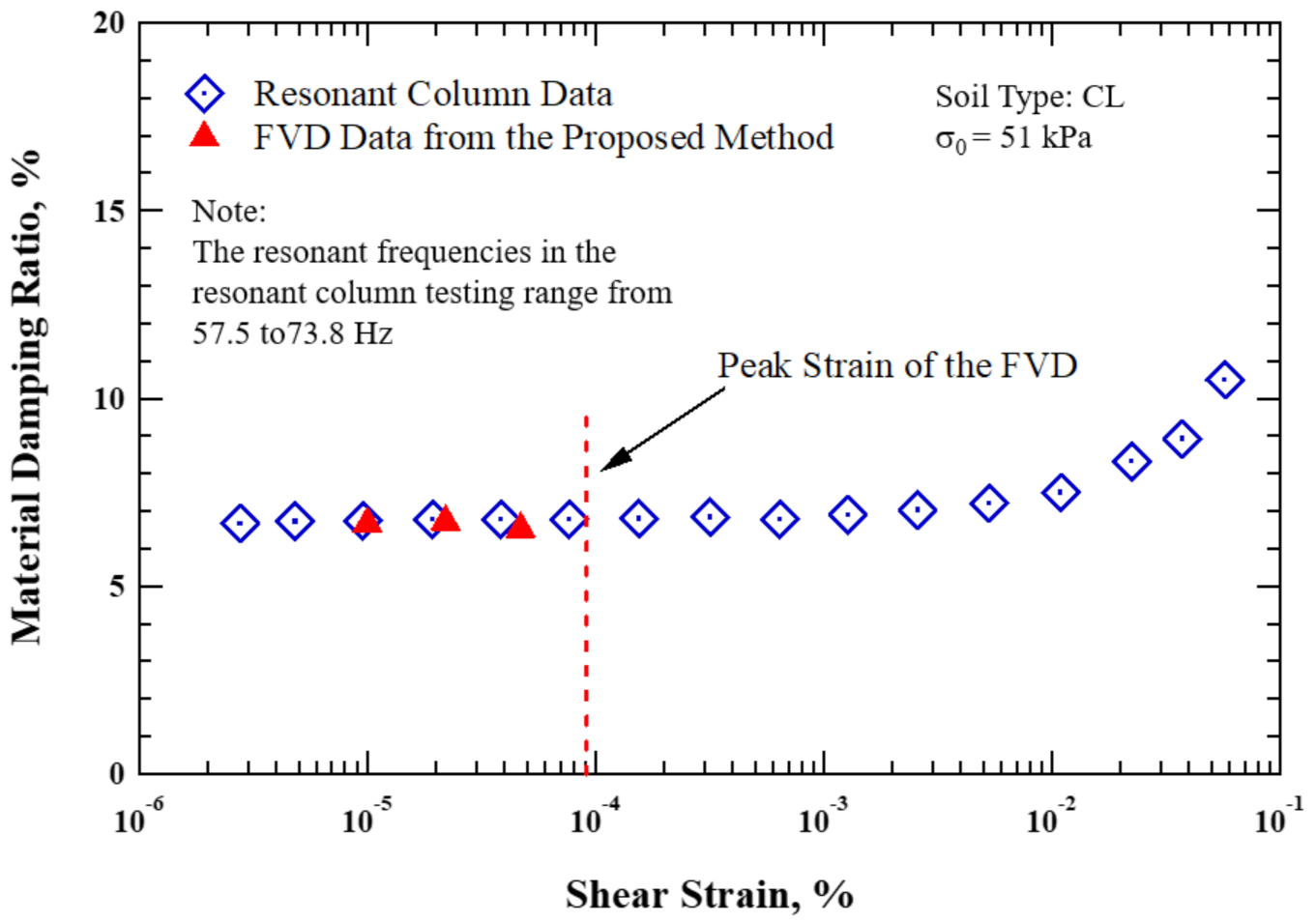
3.4. Validation of the Small-Strain Viscous Damping Ratio from the Proposed Method
4. Discussion
5. Conclusions
Author Contributions
Funding
Institutional Review Board Statement
Informed Consent Statement
Acknowledgments
Conflicts of Interest
References
- Kramer, S. Geotechnical Earthquake Engineering, 1st ed.; Prentice Hall: Hoboken, NJ, USA, 1996. [Google Scholar]
- Richart, F.E. Vibrations of Soils and Foundations; Prentice-Hall: Hoboken, NJ, USA, 1971; Volume 8. [Google Scholar]
- Menq, F. Dynamic Properties of Sandy and Gravelly Soils. Ph.D. Thesis, The University of Texas at Austin, Austin, TX, USA, 2003. [Google Scholar]
- Dobry, R.; Ladd, R.S.; Yokel, F.Y.; Chung, R.; Powell, D.J. Prediction of Pore Water Pressure Buildup and Liquefaction of Sands during Earthquakes by the Cyclic Strain Method; Report No. PB8311617; U.S. Department of Commerce: Washington, DC, USA, 1982.
- Ni, S.H. Dynamic Properties of Sand under True Triaxial Stress States from Resonant Column/Torsional Shear Tests. Ph.D. Thesis, The University of Texas at Austin, Austin, TX, USA, 1987. [Google Scholar]
- Hwang, S. Dynamic Properties of Natural Soils. Ph.D. Thesis, The University of Texas at Austin, Austin, TX, USA, 1998. [Google Scholar]
- Keene, A. Next-Generation Equipment and Procedures for Combined Resonant Column and Torsional Shear Testing. Ph.D. Thesis, The University of Texas at Austin, Austin, TX, USA, 2017. [Google Scholar]
- Wang, Y.; Stokoe, K.H. Development of Constitutive Models for Linear and Nonlinear Shear Modulus and Material Damping Relationships of Uncemented Soils. J. Geotech. Geoenvironmental Eng. 2021, in press. [Google Scholar]
- Darendeli, M. Development of A New Family of Normalized Modulus Reduction and Material Damping Curves. Ph.D. Thesis, The University of Texas at Austin, Austin, TX, USA, 2001. [Google Scholar]
- Payan, M.; Senetakis, K.; Khoshghalb, A.; Khalili, N. Influence of Particle Shape on Small-Strain Damping Ratio of Dry Sands. Geotechnique 2016, 66, 610–616. [Google Scholar] [CrossRef] [Green Version]
- Senetakis, K.; Anastasiadis, A.; Pitilakis, K. A Comparison of Material Damping Measurements in Resonant Column Using the Steady-State and Free-Vibration Decay Methods. Soil Dyn. Earthq. Eng. 2015, 74, 10–13. [Google Scholar] [CrossRef]
- Yu, S.; Shan, Y. Experimental Comparison and Study on Small-Strain Damping of Remolded Saturated Soft Clay. Geotech. Geol. Eng. 2017, 35, 2479–2483. [Google Scholar] [CrossRef]
- Tao, Y.; Rathje, E. Insights into Modeling Small-Strain Site Response Derived from Downhole Array Data. J. Geotech. Geoenvironmental Eng. 2019, 145, 04019023. [Google Scholar] [CrossRef]
- Konstadinou, M.; Georgiannou, V.N. Cyclic Behaviour of Loose Anisotropically Consolidated Ottawa Sand Under Undrained Torsional Loading. Geotechnique 2013, 63, 1144–1158. [Google Scholar] [CrossRef]
- Rix, G.J.; Meng, J. A Non-Resonance Method for Measuring Dynamic Soil Properties. Geotech. Test. J. 2005, 28, 1–8. [Google Scholar]
- Bracewell, R. The Fourier Transform and Its Applications, 3rd ed.; McGraw-Hill Higher Education: New York City, NY, USA, 1978. [Google Scholar]
- Song, B.; Tsinaris, A.; Anastasiadis, A.; Pitilakis, K.; Chen, W. Small-Strain Stiffness and Damping of Lanzhou Loess. Soil Dyn. Earthq. Eng. 2017, 95, 96–105. [Google Scholar] [CrossRef]
- Senetakis, K.; Payan, M. Small Strain Damping Ratio of Sands and Silty Sands Subjected to Flexural and Torsional Resonant Column Excitation. Soil Dyn. Earthq. Eng. 2018, 114, 448–459. [Google Scholar] [CrossRef]
- Feldman, M. Hilbert Transform Applications in Mechanical Vibration; John Wiley & Sons, Ltd.: Hoboken, NJ, USA, 2011; Volume 1. [Google Scholar]
- Facciorusso, J. An Archive of Data from Resonant Column and Cyclic Torsional Shear Tests Performed on Italian Clays. Earthq. Spectra 2021, 37, 545–562. [Google Scholar] [CrossRef]
- Kokusho, T. Cyclic Triaxial Test of Dynamic Soil Properties for Wide Strain Range. Soils Found. 1980, 3, 305–312. [Google Scholar] [CrossRef]
- Diaz-Rodriguez, J.A.; Lopez-Molina, J.A. Strain Thresholds in Soil Dynamics. In Proceedings of the 14th World Conference on Earthquake Engineering, Beijing, China, 12–17 October 2008. [Google Scholar]


| ID. | Shear Strain, % | λmin, % | |
|---|---|---|---|
| Stack | Phase-Based | ||
| 1 | 3.38 × 10⁻⁵ | 5.44 | 4.09 |
| 2 | 6.70 × 10⁻⁵ | 4.70 | 3.65 |
| 3 | 1.35 × 10⁻⁴ | 4.29 | 3.62 |
| 4 | 2.55 × 10⁻⁴ | 3.93 | 3.63 |
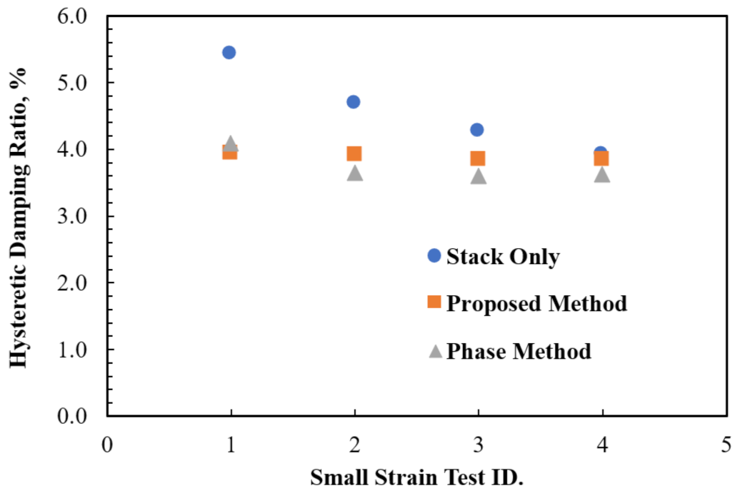
| ID. | Shear Strain, % | λmin, % | ||
|---|---|---|---|---|
| Stack | Phase Method | Proposed Method | ||
| 1 | 3.38 × 10⁻⁵ | 5.44 | 4.09 | 3.95 |
| 2 | 6.70 × 10⁻⁵ | 4.70 | 3.65 | 3.93 |
| 3 | 1.35 × 10⁻⁴ | 4.29 | 3.62 | 3.87 |
| 4 | 2.55 × 10⁻⁴ | 3.93 | 3.63 | 3.87 |
| Mean | 4.59 | 3.75 | 3.91 | |
| Standard Deviation | 0.65 | 0.23 | 0.04 | |
| Peaks | δ | Dmin, % |
|---|---|---|
| Z1/Z2 | 0.41 | 6.57 |
| Z2/Z3 | 0.37 | 5.89 |
| Z3/Z4 | 0.53 | 8.41 |
Publisher’s Note: MDPI stays neutral with regard to jurisdictional claims in published maps and institutional affiliations. |
© 2021 by the authors. Licensee MDPI, Basel, Switzerland. This article is an open access article distributed under the terms and conditions of the Creative Commons Attribution (CC BY) license (https://creativecommons.org/licenses/by/4.0/).
Share and Cite
Xu, Z.; Tao, Y.; Hernandez, L. Novel Methods for the Computation of Small-Strain Damping Ratios of Soils from Cyclic Torsional Shear and Free-Vibration Decay Testing. Geotechnics 2021, 1, 330-346. https://doi.org/10.3390/geotechnics1020016
Xu Z, Tao Y, Hernandez L. Novel Methods for the Computation of Small-Strain Damping Ratios of Soils from Cyclic Torsional Shear and Free-Vibration Decay Testing. Geotechnics. 2021; 1(2):330-346. https://doi.org/10.3390/geotechnics1020016
Chicago/Turabian StyleXu, Zhongze, Yumeng Tao, and Lizeth Hernandez. 2021. "Novel Methods for the Computation of Small-Strain Damping Ratios of Soils from Cyclic Torsional Shear and Free-Vibration Decay Testing" Geotechnics 1, no. 2: 330-346. https://doi.org/10.3390/geotechnics1020016
APA StyleXu, Z., Tao, Y., & Hernandez, L. (2021). Novel Methods for the Computation of Small-Strain Damping Ratios of Soils from Cyclic Torsional Shear and Free-Vibration Decay Testing. Geotechnics, 1(2), 330-346. https://doi.org/10.3390/geotechnics1020016