Asymmetric Seasonal Warming and Land Cover Change in a Tropical Coastal City: Multi-Temporal Evidence from Chattogram, Bangladesh

Abstract

Rapid urbanization is reshaping land surface conditions and local thermal environments in fast-growing coastal cities. This study examines how Land Use Land Cover (LULC) transformation influenced seasonal land surface temperature (LST) dynamics in Chattogram City Corporation (CCC), Bangladesh, over 2004–2024. Multi-temporal Landsat imagery was analyzed using a Random Forest classifier, and spectral indices (NDVI, NDBI, NDBaI, MNDWI) were derived to characterize surface biophysical conditions. Built-up land expanded by 27.71 km², largely replacing agricultural and vegetated areas. Summer mean LST rose from 36.08 °C to 36.50 °C, while winter LST rose from 25.25 °C to 26.97 °C. Only the winter warming trend is statistically significant; the summer change falls within the ±1–2 °C retrieval uncertainty of Landsat-derived LST. The summer–winter thermal gap consequently narrowed from 10.83 °C to 9.53 °C, indicating that urbanization-driven warming in this tropical coastal city is disproportionately concentrated in the cool dry season. Partial correlation and multiple regression analyses confirm that built-up intensity (NDBI) is the dominant driver of surface warming, while vegetation (NDVI) exerts a consistent cooling influence. Water bodies showed contrasting seasonal trends, with winter extent declining alongside a slight summer increase. These findings highlight the critical role of vegetation and water bodies in moderating urban heat and provide data-driven insights for climate-responsive planning in rapidly urbanizing coastal cities.

1. Introduction

Rapid urbanization has become a defining environmental process of the twenty-first century, reshaping land surface conditions and influencing local climatic systems worldwide. As of 2024, about 56% of the world’s population lives in urban areas, and this proportion is projected to reach 68% by 2050 [1]. The continued expansion of cities transforms natural landscapes by replacing vegetated and permeable surfaces with impervious built structures, thereby altering urban microclimates and ecological functioning. This process is particularly pronounced in South and Southeast Asia, where urban growth frequently outpaces infrastructural and environmental capacity. The conversion of natural and agricultural land to impervious surfaces modifies surface energy balance, hydrological dynamics, and local thermal regulation [2,3].

The relationship between LULC change and LST has consequently become a central concern in urban climate research. Surfaces composed of concrete, asphalt, and metal suppress evapotranspiration, increase sensible heat flux, and enhance thermal storage, producing the elevated temperatures characteristic of the urban heat island (UHI) effect, in which built environments are warmer than surrounding rural areas [4,5]. Elevated LST has been linked to greater energy demand, degraded air quality, reduced thermal comfort, and heightened heat-related health risks, effects that are most acute in rapidly developing cities where planning struggles to keep pace with growth [6,7]. Multi-temporal satellite observation, and the Landsat archive in particular, enable systematic assessment of land-cover transitions and their thermal consequences through spectral indices such as NDVI, NDBI, NDBaI, and MNDWI, which capture vegetation cover, built-up intensity, soil exposure, and surface moisture [8,9].

Studies across rapidly expanding Asian cities consistently report positive NDBI–LST and negative NDVI–LST relationships [10]. These confirm that impervious expansion intensifies surface warming, while vegetation moderates it [11,12,13]. Despite this consistency, the prevailing analytical approaches share several limitations. Many rely on single-date or single-season imagery, which conflates seasonal variability with long-term change [9,14]. Most quantify LST–index relationships through simple bivariate correlation, without controlling for the topographic, hydrological, and demographic factors that jointly influence surface temperature. Warming is also often treated as though it were uniform across seasons. As a result, the seasonal structure of urban warming has received limited attention, particularly in tropical coastal settings where maritime and monsoonal influences complicate the thermal response.

While these studies establish a clear regional precedent for LULC-driven warming, Chattogram’s setting differs from that of the commonly studied inland cities in ways that shape its thermal behavior. Inland South Asian megacities such as Dhaka and Delhi experience largely continental thermal regimes, in which summer heat accumulates with limited maritime moderation [15]. Chattogram, by contrast, occupies an unusual ecological transition zone where the Bay of Bengal coastal plain meets the foothills of the Chittagong Hill Tracts within a single urban boundary, bringing marine, riverine, agricultural, and forested-hill ecosystems into close juxtaposition and supporting exceptional biological diversity [16]. This convergence gives the city the character of a tropical coastal–hill ecosystem, shaped by the Bay of Bengal sea breeze, persistent humidity, and the South Asian monsoon [17]. Its pattern of urban growth is correspondingly distinctive: development is confined between the eastern hills and the western coastline, producing dense, linear, topographically channeled expansion rather than the radial growth typical of inland megacities. These ecological, climatic, and morphological characteristics generate land–atmosphere interactions not represented in inland or temperate–subtropical cities, and they motivate region-specific analysis of LULC–LST dynamics in Chattogram.

As Bangladesh’s principal seaport and second-largest commercial center, Chattogram handles more than 80% of the country’s international trade and contributes approximately 12% of the national GDP [18]. Rapid industrialization and population growth, with the district population reaching about 9.17 million at an annual growth rate of 2.06% [19], have accelerated land conversion within and around the city, reducing the vegetation and water bodies that historically moderated its thermal environment. Urban thermal dynamics unfold across diurnal, seasonal, and interannual-to-decadal scales. Most South Asian studies have relied on single-date imagery or annual averages, limiting their ability to distinguish seasonal variability from long-term urban warming. A multi-temporal framework that explicitly separates these temporal scales provides a more robust basis for attributing observed thermal change to its underlying drivers.

Despite Chattogram’s (formerly known as Chittagong) economic significance and rapidly changing landscape, detailed assessments linking long-term land-cover change to seasonal LST dynamics remain scarce; existing Bangladeshi studies have generally examined urban expansion or LST trends in isolation [14]. Three gaps in particular persist. First, the seasonal structure of urban warming, whether warming is uniform across seasons or concentrated in particular ones, has rarely been tested in tropical coastal cities, despite the strong seasonal control that climate exerts on surface temperature (ST). Second, the combined explanatory power of multiple spectral indices (NDVI, NDBI, NDBaI, MNDWI) for seasonal LST, evaluated while controlling for confounding factors such as elevation, distance to water, and population density, has not been assessed in Chattogram. Third, the specific land-cover transition pathways that drive thermal intensification have not been quantified over multi-decadal periods.

This study addresses these gaps through a multi-season, multi-decadal analysis of CCC spanning 2004–2024. It integrates Random Forest LULC classification, spectral index analysis, and a controlled statistical framework, combining bivariate correlation, partial correlation, and multiple regression, to isolate the independent thermal contribution of each surface index, and applies trend testing to evaluate the significance of observed change. The specific objectives are as follows:

• Measure seasonal and interannual changes in LULC within CCC from 2004 to 2024.
• Analyze the spatial and temporal characteristics of LST during both the summer and winter seasons.
• Evaluate statistical relationships between LST and key geospatial indicators, including NDVI, NDBI, NDBaI, and MNDWI.
• Examine how different LULC categories correspond to variations in surface temperature distribution.
• Determine the primary land-cover transition pathways responsible for the observed thermal changes.

2. Materials and Methods

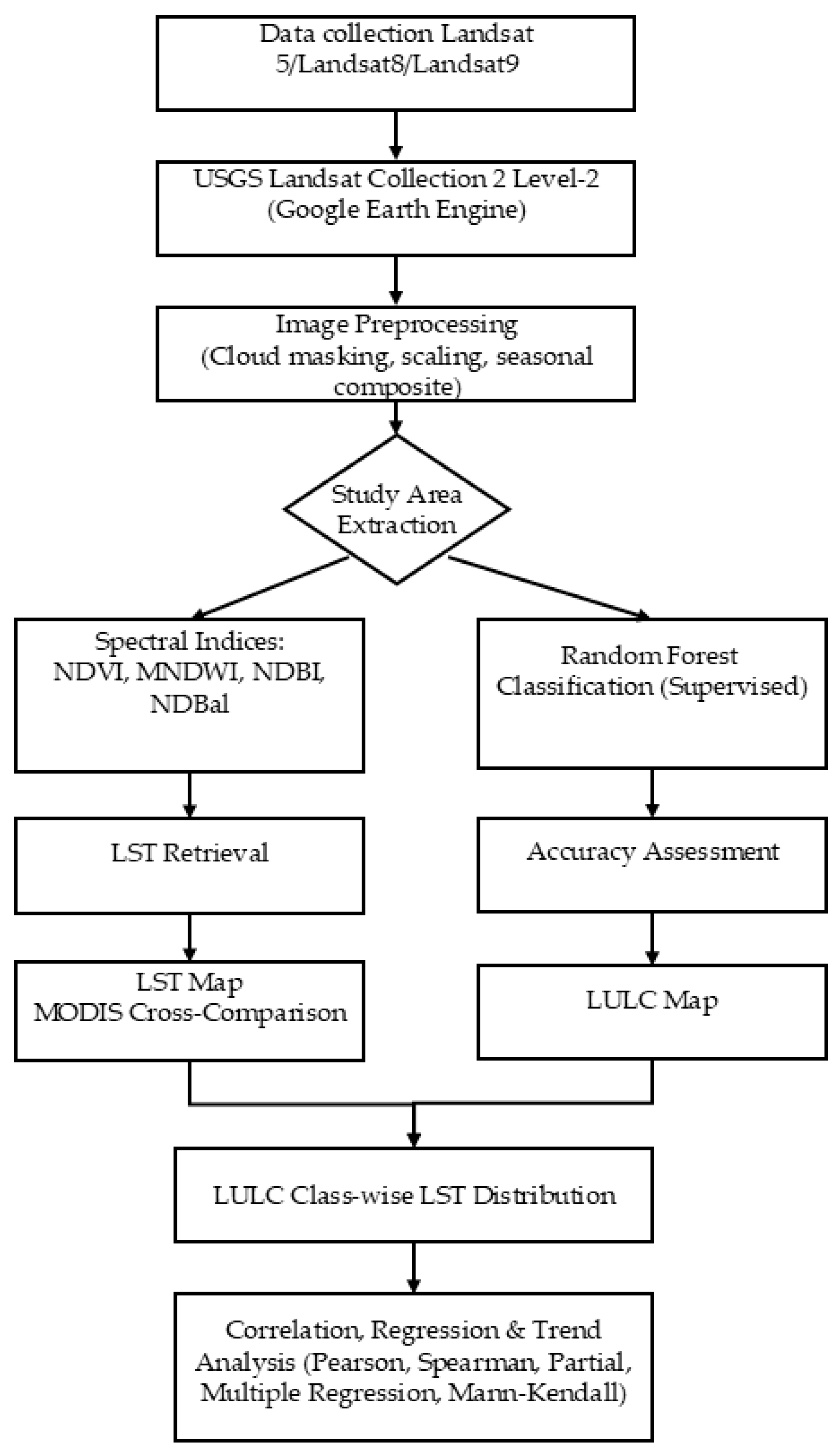
The methodological framework integrates multi-temporal Landsat imagery, LULC classification, spectral index analysis, LST characterization, and statistical modeling to investigate seasonal LULC–LST relationships in CCC. Image acquisition, cloud masking, seasonal compositing, spectral index computation, Random Forest classification, and LST extraction were all performed within the Google Earth Engine (GEE) cloud computing platform (Google LLC, Mountain View, CA, USA), while the subsequent correlation, regression, and trend analyses were carried out in ArcGIS Pro 10.4.1. Following Figure 1, Landsat imagery was first accessed as analysis-ready Collection 2 Level-2 products and subjected to cloud masking, scaling, and seasonal compositing.

The study area was then extracted, after which the analysis proceeded along two parallel streams: the first computed the spectral indices (NDVI, MNDWI, NDBI, NDBaI) and extracted LST to generate seasonal LST maps, while the second performed RF classification followed by accuracy assessment to produce LULC maps. The two outputs were combined to derive the LULC class-wise LST distribution, and correlation, regression, and trend analyses were then applied to quantify the relationships between LST and the surface indices.

2.1. Study Area

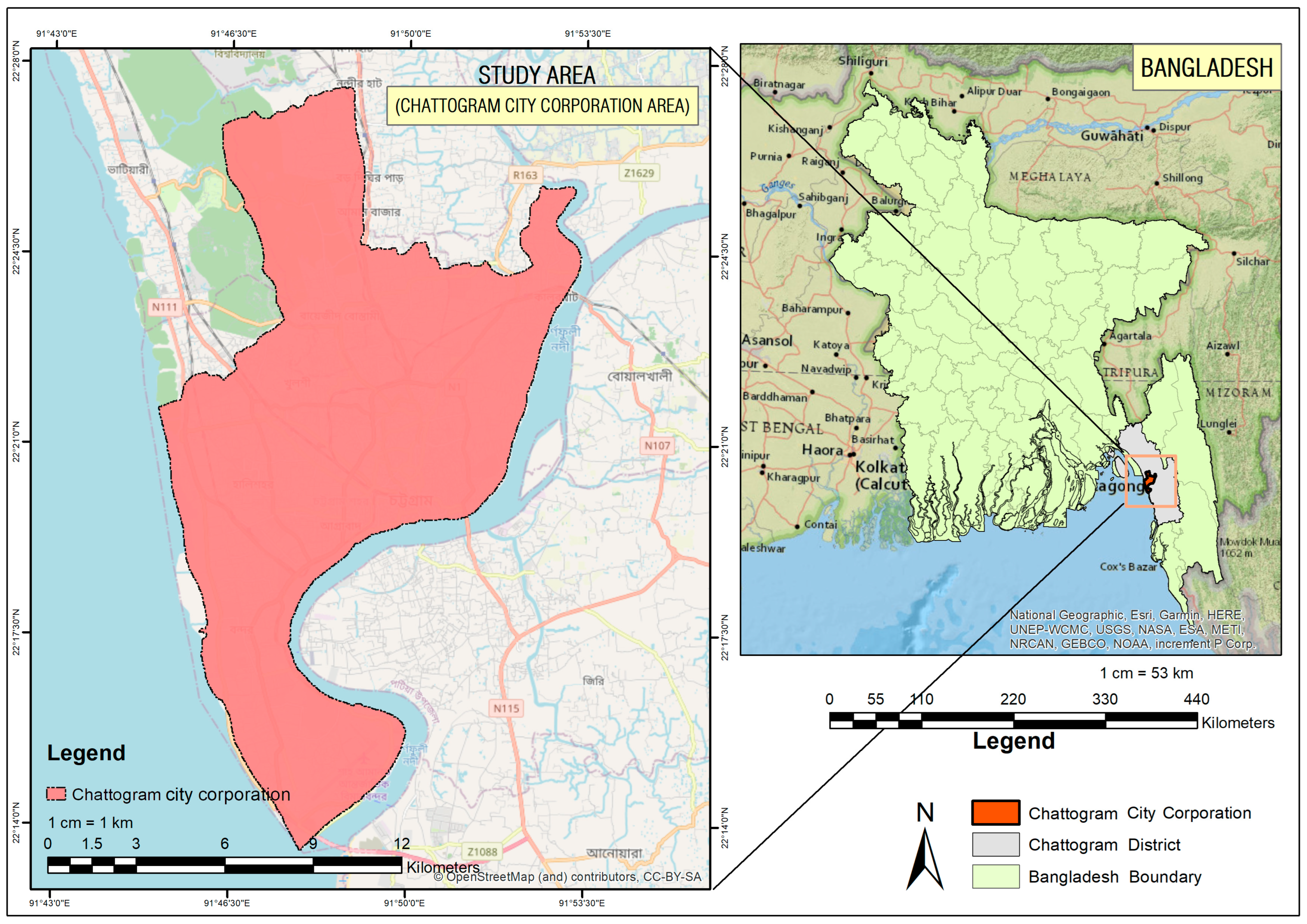
CCC is located in the southeastern coastal region of Bangladesh, between 21°54′–22°59′ N and 91°17′–92°13′ E (Figure 2). As the country’s principal seaport and second-largest metropolitan area, it plays a central role in international trade, industrial production, and economic development. The surrounding district covers approximately 5282.92 km², bordered by hilly terrain to the east, Cox’s Bazar to the south, Tripura (India) to the north, and the Noakhali district and the Bay of Bengal to the west [20]. Within this broader district, the administrative boundary of CCC, which defines the study area, encompasses approximately 169.67 km². The topography is heterogeneous, comprising flat coastal plains in the west, undulating terrain in the center, and forested hills in the east, with hills accounting for roughly 35% of the district area and vacant land about 12% [20].

These varied landscapes produce complex land surface–atmosphere interactions that shape local microclimatic conditions. The region has a tropical monsoon climate (Köppen: Am), characterized by a short dry season and pronounced summer monsoon rainfall, within the broader Bangladeshi seasonal cycle of summer (pre-monsoon), monsoon, post-monsoon, and winter [14]. Two climatically contrasting seasons were selected to capture the extremes of thermal behavior, corresponding to the periods of maximum and minimum surface thermal stress and least affected by the persistent cloud cover that makes consistent multi-year compositing infeasible during the monsoon and post-monsoon periods.

During summer (March–June), average temperatures range from 22 to 32 °C under high solar radiation, elevated evaporative demand, and declining pre-monsoon soil moisture. This period typically records the highest ST and represents peak urban heat stress. During winter (November–February), average temperatures range from 22 to 26 °C under reduced atmospheric moisture, stable anticyclonic conditions, and minimal precipitation [21].

Annual precipitation ranges from approximately 2400–3000 mm, of which nearly 80% falls during the May–September monsoon [19], strongly influencing surface moisture, vegetation growth, and thermal response across land cover types. The district population has reached approximately 9,169,465, growing at 2.06% annually [19], driven by migration linked to port operations, manufacturing, and services. To accommodate this growth, the city has expanded horizontally toward the north, east, and south, progressively converting natural and agricultural land into built-up surfaces. The analysis spans a twenty-year period (2004–2024), with an intermediate observation in 2014, chosen to capture the early, middle, and recent phases of CCC’s accelerated urbanization at approximately even decadal intervals, while ensuring the availability of cloud-free imagery in a persistently humid coastal environment.

2.2. Data and Preprocessing

Land surface conditions were characterized using Landsat Collection 2 Level-2 products (U.S. Geological Survey EROS Center, Sioux Falls, SD, USA), accessed and processed within GEE (Table S1). Imagery was drawn from Landsat 5 TM for 2004, Landsat 8 OLI/TIRS for 2014, and Landsat 9 OLI-2/TIRS-2 for 2024, all at 30 m spatial resolution and covering the study area within WRS-2 path 136, rows 44–45. Collection 2 Level-2 products are delivered as terrain and atmospherically corrected surface reflectance together with an ST band, so that radiometric calibration and atmospheric correction are already applied by the USGS [22,23]. This ensures consistent, reproducible inputs across the three sensors and removes the need for user-applied correction. For each year and season, a single representative image was produced by pixel-wise mean compositing of all qualifying cloud-free scenes within the seasonal window (summer: March–June; winter: November–February). Cloud and cloud-shadow pixels were first masked using the Level-2 quality-assessment bands, and only scenes with less than 5% cloud cover over the study area were retained. Each seasonal composite drew on multiple scenes rather than a single acquisition, which reduces the influence of transient atmospheric conditions and short-term meteorological variability. All composites were clipped to the CCC administrative boundary prior to analysis, and the resulting composites are summarized in

Table 1. Characteristics of the Landsat seasonal composites used for LULC classification, spectral index calculation, and LST extraction.

Year	Season	Satellite/Sensor	Collection	Seasonal Window	Composite Method	WRS Path/Row	Spatial Resolution
2004	Summer	Landsat 5 TM	Collection 2 Level-2	Mar–Jun	Pixel-wise mean	136/044–045	30 m
2004	Winter	Landsat 5 TM	Collection 2 Level-2	Nov–Feb	Pixel-wise mean	136/044–045	30 m
2014	Summer	Landsat 8 OLI/TIRS	Collection 2 Level-2	Mar–Jun	Pixel-wise mean	136/044–045	30 m
2014	Winter	Landsat 8 OLI/TIRS	Collection 2 Level-2	Nov–Feb	Pixel-wise mean	136/044–045	30 m
2024	Summer	Landsat 9 OLI-2/TIRS-2	Collection 2 Level-2	Mar–Jun	Pixel-wise mean	136/044–045	30 m
2024	Winter	Landsat 9 OLI-2/TIRS-2	Collection 2 Level-2	Nov–Feb	Pixel-wise mean	136/044–045	30 m

.

2.3. LULC Classification

Five LULC classes were defined according to their distinct spectral characteristics and their relevance to surface thermal behavior: Built-up (BU), Vegetation (VG), Agricultural land (AL), Bare land (BL), and Water body (WB) [24]. These classes represent the principal surface types governing LST variability in the coastal urban environment. Training samples were selected by visual interpretation of false-color composites (NIR–Red–Green), supported by high-resolution Google Earth imagery, with separate training sets prepared for summer and winter to accommodate seasonal differences in vegetation phenology and crop cycles.

Classification was performed using the RF algorithm, implemented in Google Earth Engine through the ee.Classifier.smileRandomForest function [25,26]. RF is a non-parametric ensemble classifier that builds many decision trees from bootstrap samples of the training data and assigns each pixel by majority vote. It was chosen in preference to parametric classifiers such as the Maximum Likelihood Classifier because it makes no assumption of multivariate normality—an assumption frequently violated across the spectrally mixed surfaces of tropical cities—and because it consistently outperforms such classifiers in heterogeneous urban landscapes. The classifier used all available spectral bands as inputs, with the number of trees set to 500 and the number of variables sampled at each split set to the square root of the number of inputs, following standard practice.

Classification accuracy was assessed using confusion matrices based on 203–300 independent, stratified validation points per image, with reference labels assigned through visual interpretation of high-resolution imagery. Overall accuracy ranged from 87.00% to 94.58% and the Kappa coefficient from 83.24% to 92.45%, indicating substantial to near-perfect agreement and exceeding the 85% threshold commonly regarded as reliable for LULC mapping. The associated 95% confidence intervals (

Table 2. Overall accuracy, Kappa coefficient, and 95% confidence intervals for the six LULC classification outputs.

LULC Map (Year–Season)	Validation Points (n)	Correct Samples	OA (%)	Kappa (%)	95% CI Lower (%)	95% CI Upper (%)
Summer 2004	229	211	92.14	89.44	88.65	95.63
Summer 2014	235	211	89.79	86.46	85.92	93.66
Summer 2024	252	224	88.89	85.57	85.01	92.77
Winter 2004	214	188	87.85	83.81	83.47	92.23
Winter 2014	203	192	94.58	92.45	91.47	97.70
Winter 2024	300	261	87.00	83.24	83.19	90.81

) confirm that accuracy remained within statistically acceptable limits across all six classifications.

2.4. Spectral Indices

Four spectral indices were computed in GEE at 30 m resolution for each seasonal composite to represent the biophysical properties governing surface thermal behavior: the NDVI for vegetation density and vigor [27]; the NDBI for impervious-surface intensity [28]; the NDBaI for exposed and bare soil [29]; and the MNDWI for surface water [30]. These indices were applied using their original formulations, with band assignments following the standard Landsat 5, 8, and 9 mappings. NDVI values range from −1 to +1, with negative values indicating water, values near zero indicating built-up or bare surfaces, and higher positive values indicating progressively denser vegetation [31]. To support the class-wise LST analysis, the NDVI ranges corresponding to each LULC type were adopted from [32] and are listed in

Table 3. NDVI value ranges indicating different LULC types used for LST distribution [32].

Sl. No.	Class	NDVI Range
1	Water	−0.28 to −0.015
2	Built-up	−0.014 to +0.13
3	Barren Land	+0.14 to +0.18
4	Agriculture land	+0.19 to +0.27
5	Vegetation	+0.27 to +0.36
6	Dense vegetation	+0.36 to +0.74

.

2.5. Land Surface Temperatures

LST was obtained directly from the Landsat Collection 2 Level-2 ST band, which provides per-pixel LST derived by the USGS single-channel algorithm using ASTER GED emissivity and atmospheric-profile inputs [22,23,33]. The ST band was rescaled to degrees Celsius and composited for each season using the same pixel-wise mean procedure applied to the reflectance data. Relying on the operational Level-2 ST product yields a physically consistent and fully reproducible LST estimate across the three sensors and avoids the additional uncertainty that a manual, emissivity-dependent retrieval would introduce. The spatial reliability of the resulting LST is examined independently in Section 2.6 through cross-comparison with the MODIS MOD11A2 product.

2.6. MODIS LST Cross-Comparison Method

To assess the spatial consistency of the Landsat-derived LST, an independent cross-comparison was performed using MODIS MOD11A2 Version 6.1 eight-day daytime LST product (Terra platform, LST_Day_1km band, quality-screened with the accompanying QC_Day band) [34] (Table S1). Because MODIS has a coarser spatial resolution (1 km) than Landsat (30 m), the Landsat LST was aggregated to the MODIS grid before comparison, and bias, mean absolute error (MAE), root mean square error (RMSE), Pearson’s correlation coefficient (r), and the coefficient of determination (R²) were computed from the matched valid pixels of each seasonal composite.

This comparison evaluates the agreement in spatial temperature patterns between two independent satellite products rather than the absolute accuracy of either. MODIS LST is itself a remotely sensed product with its own retrieval uncertainties and cannot substitute for in situ ST measurements; the comparison is, therefore, best understood as an assessment of spatial consistency rather than validation against ground truth. Continuous meteorological observations spanning the full 2004–2024 period were unavailable, and direct ground-based validation was consequently not possible. The results of this comparison are reported in Section 3.4.

2.7. Uncertainty Quantification

Both the LULC classification and the LST estimates carry inherent uncertainties that may influence the significance of the observed trends. Classification accuracy was quantified with 95% confidence intervals derived from the binomial approximation (Table 2), based on 203–300 validation points per image. Class-wise results indicate that built-up, vegetation, and agricultural land were classified with high reliability, whereas the lower accuracy occasionally observed for bare land and water reflects spectral confusion among exposed soil, impervious surfaces, shallow water, and moist agricultural fields. The small within-year differences in classified built-up areas between summer and winter (Section 3.1) similarly reflect this classification uncertainty, rather than any genuine seasonal change in the extent of built structures.

For LST, the principal uncertainties arise from the operational retrieval itself, including sensor calibration, the atmospheric and emissivity inputs used by the USGS single-channel algorithm, residual cloud and aerosol effects, and mixed-pixel conditions at 30 m resolution. Because LST also varies with acquisition time and antecedent weather, and because each seasonal value is derived from a composite of scenes acquired within a defined window rather than from continuous observation, the reported temperatures represent characteristic seasonal surface conditions rather than climatological means. In the absence of continuous ground measurements, the expected uncertainty of the Landsat ST product is on the order of ±1.0–2.0 °C, consistent with widely reported ranges for single-channel thermal retrievals [33,35]. Differences of this magnitude were therefore interpreted with caution, while consistent spatial patterns and long-term trends were treated as more robust. This explicit treatment of uncertainty follows recent recommendations for transparent error reporting in urban land-surface assessment [36].

2.8. Statistical Analysis

Relationships between the surface indices and LST were examined using bivariate correlation, partial correlation, and multiple regression, all performed in ArcGIS Pro. A fixed sampling framework of 1125 points was applied; after removal of No-Data and edge-affected cells, 1082 valid points were retained, yielding 6491 observations across the six year–season cases. Points were allocated by stratified random sampling in proportion to the average class area, subject to a minimum threshold ensuring adequate representation of smaller classes, giving built-up (350), agriculture (300), vegetation (275), bare land (125), and water bodies (75). Using identical locations across all years and seasons ensured that the observed relationships reflected genuine spatial and temporal variation rather than differences in sampling. LST served as the dependent variable, with NDVI, NDBI, NDBaI, and MNDWI as explanatory variables. Elevation, distance to water, and population density were included as spatial controls, and year and season as temporal controls, because these factors could otherwise confound the apparent relationship between an individual index and LST; their inclusion allows for the independent contribution of each index to be isolated. Pearson’s correlation coefficient quantified linear associations and Spearman’s rank coefficient captured monotonic relationships without assuming linearity or normality. Partial correlations were then computed to isolate the association of each index with LST after controlling for the remaining covariates, and a multiple linear regression model quantified the joint and independent contributions of all predictors, with performance evaluated through the coefficient of determination (R²) and 95% confidence intervals for each coefficient. Significance was assessed at p < 0.01.

To evaluate the significance of temporal change, the Mann–Kendall trend test and Sen’s slope estimator [37] were applied to the seasonal LST and LULC-area sequences. Because only three observation years were available, the Mann–Kendall results were interpreted with caution and supplemented by two-sample mean-difference tests between 2004 and 2024, with 95% confidence intervals computed for all reported changes in mean LST (°C) and LULC area (% and km²). The resulting trends were interpreted in the context of the ±1–2 °C LST uncertainty discussed in Section 2.7.

3. Results

3.1. Seasonal Variability of LULC Distribution (2004–2024)

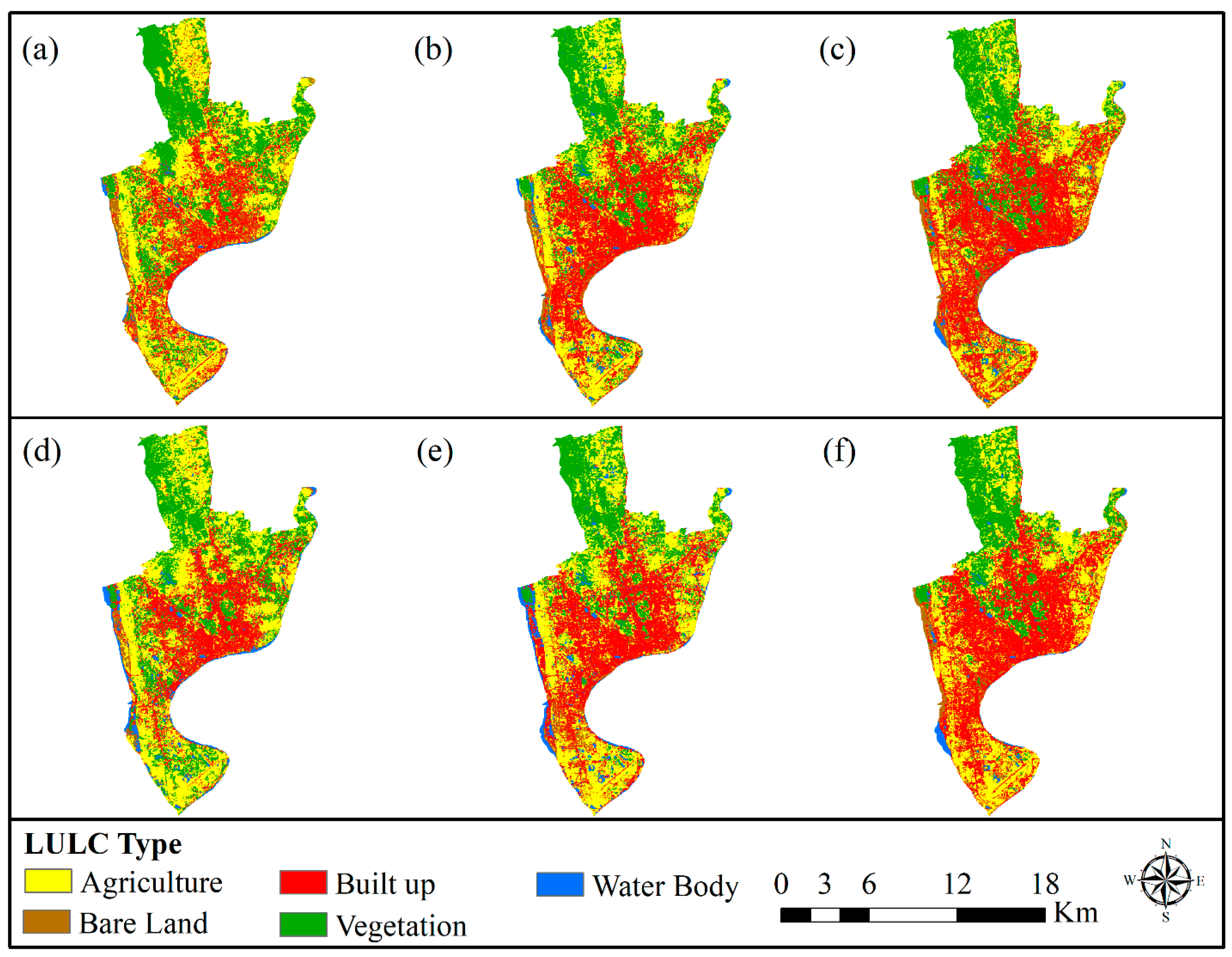
The classification results reveal substantial landscape transformation within the CCC over the twenty-year period. Figure 3 shows the spatial distribution of LULC classes for both seasons, and the corresponding class areas are summarized in

Table 4. Classified LULC statistics of CCC summer (S) and winter (W) (areas in % of mapped CCC area, 169.67 km²).

Class	2004		2014		2024		Δ S (%/km2)	Δ W (%/km2)
	S	W	S	W	S	W	S	W
Agriculture	38.42	39.48	32.06	36.03	24.21	30.02	−14.21/−24.11	−9.46/−16.05
Bare Land	7.55	5.30	5.53	5.32	10.84	5.39	+3.29/+5.58	+0.09/+0.15
Built-up	23.08	23.50	33.40	33.13	39.41	40.58	+16.33/+27.71	+17.08/+28.98
Vegetation	29.94	28.40	26.41	21.04	23.83	22.54	−6.11/−10.37	−5.86/−9.94
Water	1.01	3.32	2.60	4.48	1.71	1.47	+0.70/+1.19	−1.85/−3.14
Total	100	100	100	100	100	100

Note: The within-year differences in built-up areas between summer and winter reflect pixel-based classification uncertainty rather than genuine seasonal change in built-up extent; the summer-derived value is used as the reference estimate for long-term change.

.

In 2004, agricultural land was the dominant land-cover type, followed by vegetation, whereas built-up land occupied a considerably smaller proportion of the study area (Table 4). Although modest seasonal differences were observed among individual classes, the overall land-cover structure was similar in summer and winter, providing a consistent baseline for evaluating long-term landscape transformation.

The classified areas of several land-cover types differ modestly between the summer and winter images of a given year, and these differences require interpretation before the long-term trends are examined. For water bodies, agricultural land, and bare land, much of the seasonal variation genuinely reflects the region’s monsoon hydrology: post-monsoon winter imagery captures elevated river levels, residual floodplain water, and moist agricultural fields, whereas pre-monsoon summer imagery records lower river discharge and drier surfaces. For the built-up class, however, the small within-year differences (Table 4) are not physical; they arise from the spectral behavior of the surface rather than from any change in the urban fabric. In the drier winter months, sparse vegetation and exposed soil become spectrally more like impervious surfaces, so a proportion of mixed pixels are assigned to the built-up class. In the more vegetated and moister summer scenes, some of the same pixels are instead classified as vegetation or bare land. These classification errors are distributed differently between seasons. Together with the per-image accuracy reported in Table 2, this accounts for the observed seasonal fluctuation in built-up area. To maintain internal consistency, the long-term change analysis reported below is anchored to the summer classifications, with the winter results retained to characterize seasonal variation in surface condition and its influence on LST.

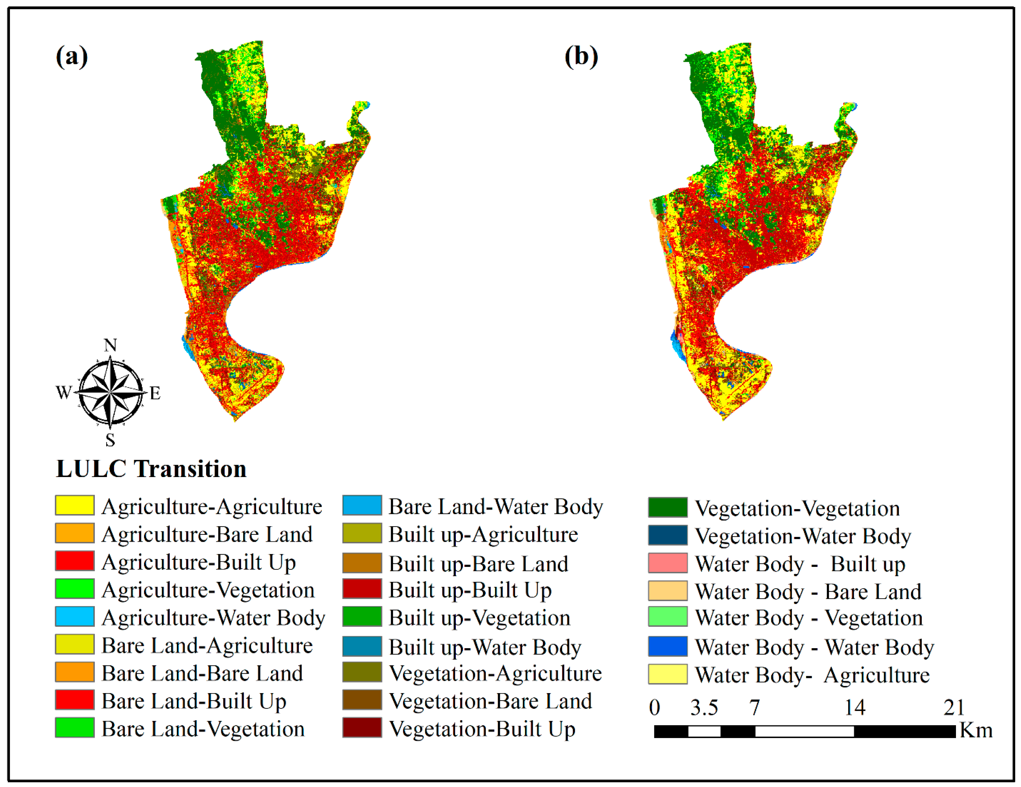
By 2024, the spatial structure of the city had changed considerably. Built-up land had become the dominant class, expanding by 27.71 km² relative to 2004, largely at the expense of agricultural land and vegetation. Bare land increased modestly, reflecting continued clearing and construction in the developing periphery. Water bodies followed contrasting seasonal trajectories, with winter extent declining as wetlands were progressively encroached upon and drained (Table 4). The transition matrix (

Table 5. LULC transition matrix in CCC during 2004–2024.

LULC Transition	Transformed Area (Summer)		Transformed Area (Winter)
	km2	%	km2	%
Agriculture → Agriculture	25.47	15.01	32.66	19.25
Agriculture → Bare Land	6.77	3.99	9.33	5.50
Agriculture → Built-up	22.53	13.28	26.59	15.67
Agriculture → Vegetation	9.55	5.63	5.78	3.41
Agriculture → Waterbody	0.66	0.39	0.63	0.37
Bare Land → Agriculture	1.15	0.68	1.34	0.79
Bare Land → Bare Land	2.75	1.62	3.23	1.90
Bare Land → Built-up	7.43	4.38	6.38	3.76
Bare Land → Vegetation	0.68	0.40	0.44	0.26
Bare Land → Waterbody	0.66	0.39	0.53	0.31
Built-up → Agriculture	2.58	1.52	1.31	0.77
Built-up → Bare Land	3.76	2.22	2.21	1.30
Built-up → Built-up	27.06	15.95	25.31	14.92
Built-up → Vegetation	2.68	1.58	0.32	0.19
Built-up → Waterbody	0.72	0.42	0.21	0.12
Vegetation → Agriculture	12.15	7.16	14.21	8.38
Vegetation → Bare Land	3.95	2.33	1.85	1.09
Vegetation → Built-up	8.73	5.14	8.81	5.20
Vegetation → Vegetation	27.80	16.38	21.84	12.87
Vegetation → Waterbody	0.57	0.34	0.62	0.37
Waterbody → Agriculture	0.14	0.08	0.47	0.28
Waterbody → Bare Land	0.60	0.35	1.80	1.06
Waterbody → Built-up	0.16	0.09	1.34	0.79
Waterbody → Vegetation	0.07	0.04	0.36	0.21
Waterbody → Waterbody	0.84	0.50	2.10	1.24
Total	169.67	100.00	169.67	100.00

, Figure 4) clarifies the pathways underlying these changes.

The dominant pathway was the conversion of agricultural land to built-up surfaces, followed by smaller contributions from vegetation-to-built-up and bare-land-to-built-up conversion (Table 5). Vegetation-to-agriculture transitions were also substantial, occurring mainly in peri-urban zones, alongside minor but environmentally significant losses of water bodies to built-up and bare land. Collectively, these transitions show that rapid urban growth, driven by population pressure and industrial development, has fundamentally reshaped the spatial structure of CCC between 2004 and 2024.

3.2. Seasonal Variability of Land Use Indices (2004–2024)

3.2.1. Built-Up Surface Dynamics (NDBI)

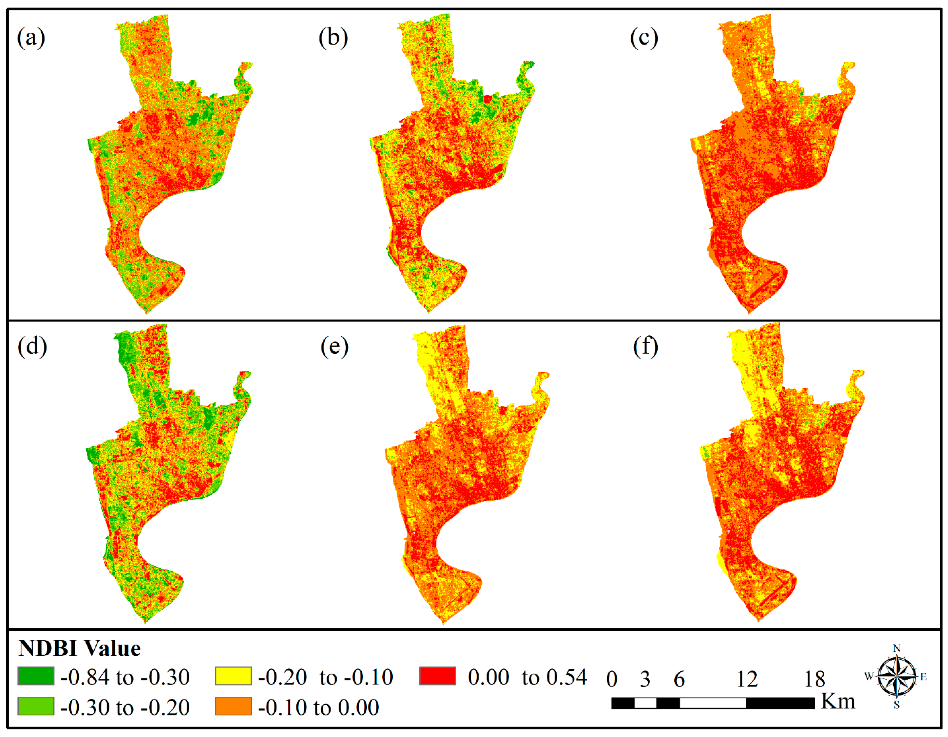
Positive NDBI values expanded progressively across both seasons, indicating continuous growth of impervious surfaces, whereas strongly negative values became increasingly rare (

Table 6. Percentage distribution of spectral index ranges across study years and seasons.

Index Range	2004		2014		2024
	S	W	S	W	S	W
NDBI
−0.84 to −0.30	3.41	7.77	2.80	0.00	0.04	0.01
−0.30 to −0.20	19.93	26.60	12.09	0.54	0.97	0.81
−0.20 to −0.10	14.89	24.26	28.68	21.71	8.75	21.93
−0.10 to 0.00	48.26	26.01	35.08	54.82	57.83	48.30
0.00 to 0.54	13.51	15.39	21.35	22.93	32.46	28.97
NDBaI
−0.40 to −0.20	0.00	0.04	0.01	0.02	0.01	0.00
−0.20 to −0.10	6.61	7.70	7.00	8.99	6.13	7.46
−0.10 to 0.00	82.79	76.49	82.39	81.37	83.87	79.99
0.00 to 0.20	10.59	15.76	10.60	9.61	9.99	12.53
0.20 to 0.40	0.01	0.01	0.01	0.00	0.00	0.01
MNDWI
−0.75 to −0.35	40.48	24.01	33.16	0.00	0.00	0.00
−0.35 to −0.10	56.04	70.21	63.08	80.75	88.62	78.31
−0.10 to 0.15	2.35	3.61	2.73	18.37	11.04	21.08
0.15 to 0.40	0.77	1.20	0.87	0.89	0.34	0.61
0.40 to 0.90	0.37	0.97	0.16	0.00	0.00	0.00
NDVI
−0.30 to −0.10	0.22	0.78	0.13	0.32	0.08	0.00
−0.10 to 0.10	2.93	6.78	14.61	22.90	25.29	25.12
0.10 to 0.30	38.24	39.51	76.61	69.88	70.36	65.90
0.30 to 0.50	48.40	44.69	8.69	6.93	4.30	9.02
0.50 to 0.80	10.22	8.29	0.00	0.00	0.00	0.00

). These patterns reflect the gradual replacement of vegetated and water-covered areas by urban land (Figure 5).

3.2.2. Bare Land Dynamics (NDBaI)

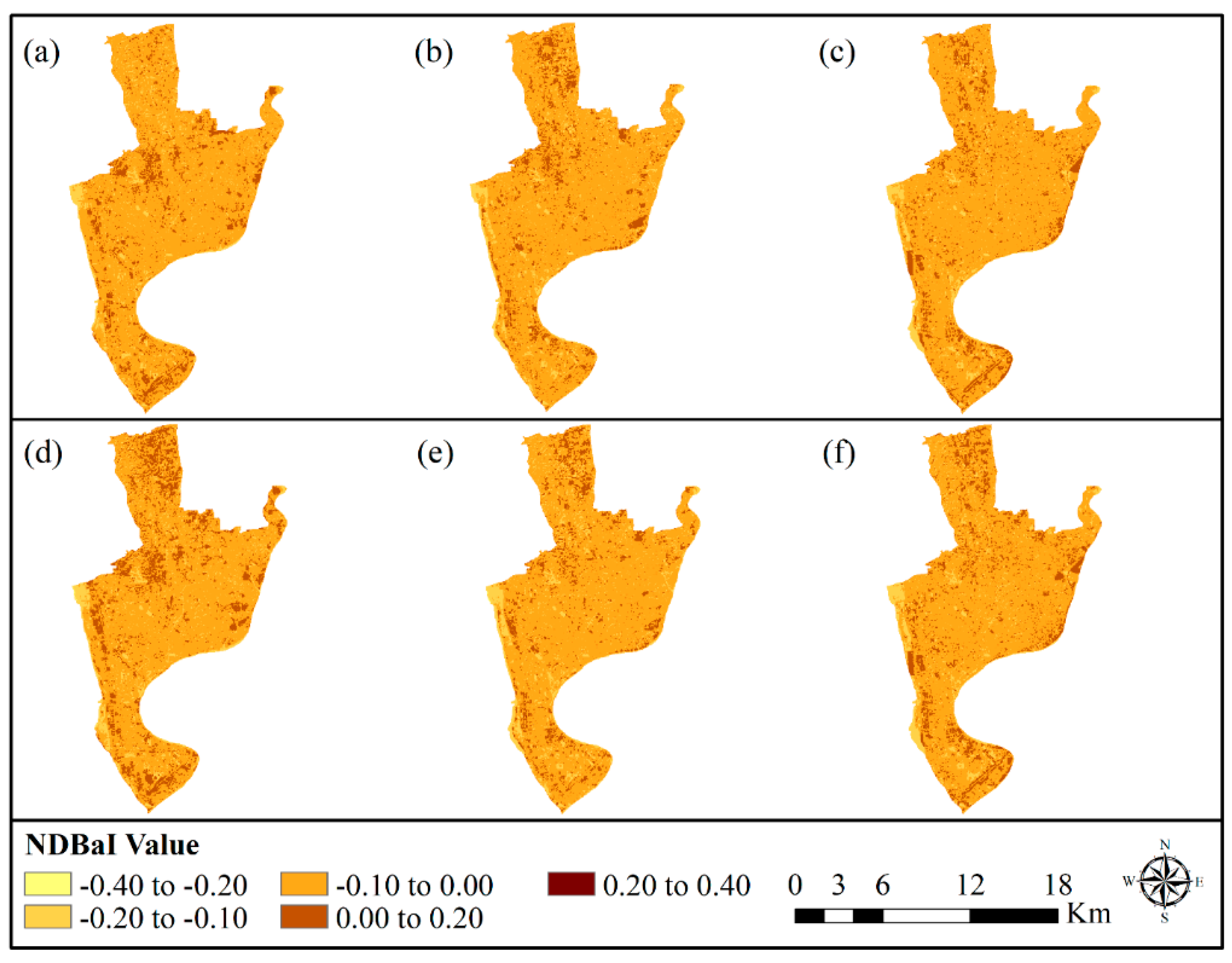
Bare land remained concentrated in transitional peri-urban areas undergoing active development (Figure 6). Although the overall NDBaI distribution changed only modestly (Table 6), this indicates that exposed soil primarily represented temporary construction phases before conversion to built-up land.

3.2.3. Surface Water Dynamics (MNDWI)

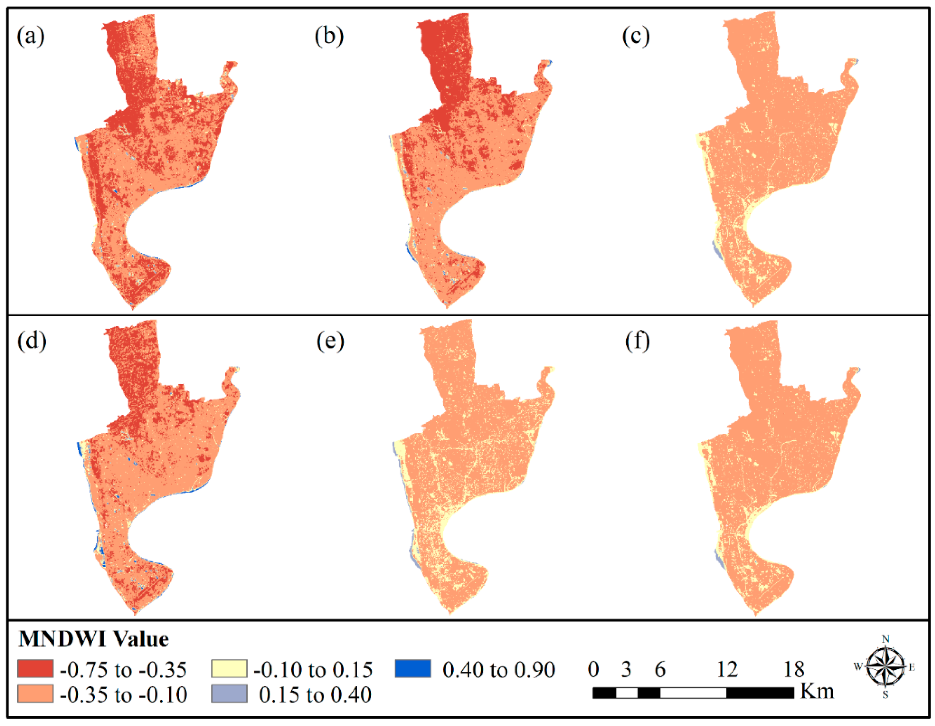
MNDWI indicates a gradual reduction in open water surfaces across the study period (Figure 7), consistent with progressive encroachment and modification of wetlands during urban expansion. The decline was most pronounced by 2024, when the highest-value class associated with permanent water bodies had almost entirely disappeared (Table 6), pointing to a continuing loss of surface-water availability.

3.2.4. Vegetation Dynamics (NDVI)

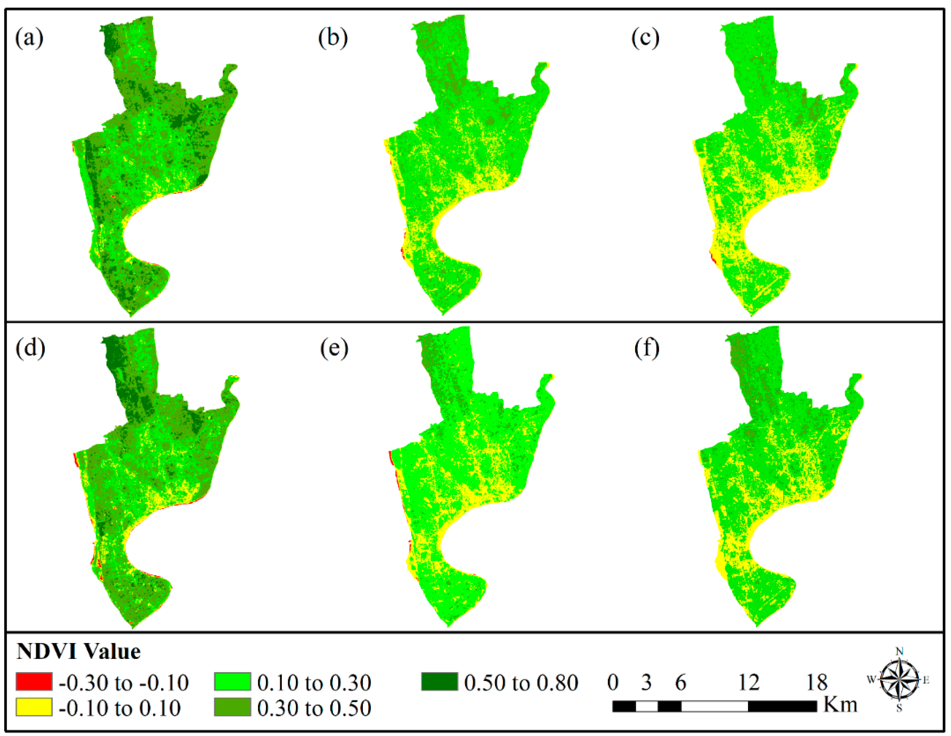
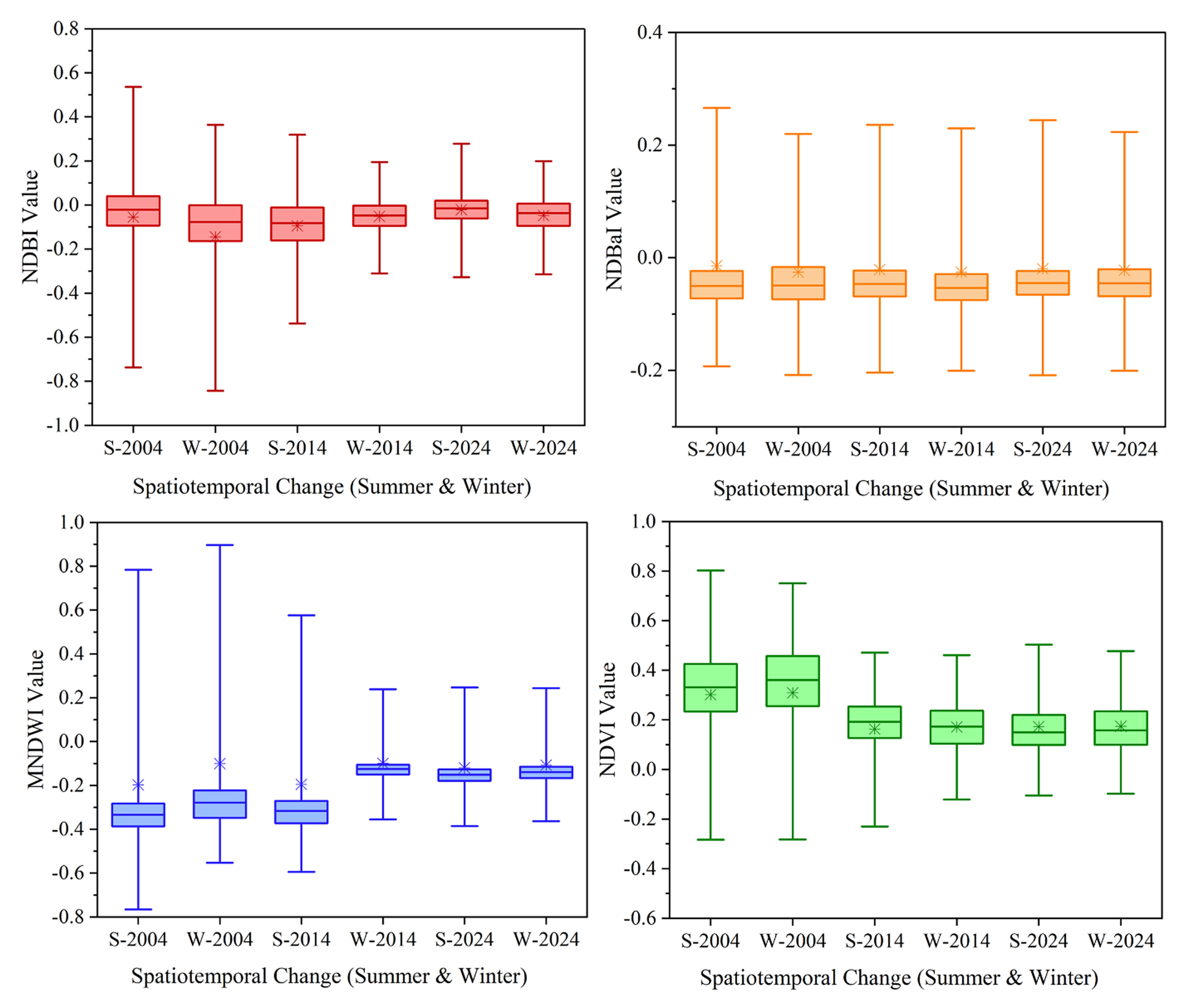
NDVI demonstrates a clear long-term reduction in vegetation cover across both seasons (Figure 8). High-NDVI areas progressively contracted, while low-NDVI classes expanded (Table 6), indicating the continued replacement of vegetated surfaces by impervious urban land. A modest rebound in mean summer NDVI is nonetheless apparent between 2014 and 2024 (Figure 9).

This is likely to reflect several factors. Interannual variation in pre-monsoon rainfall and soil moisture affects the vigor of the seasonal crops and grasses captured in the summer composites. Some vegetation also persists or partially regenerates within remnant hill pockets, urban green spaces, and intra-urban agricultural plots. Minor classification noise at mixed built-up–vegetation boundaries contributes as well. Despite this localized recovery, the overall NDVI distribution continues to shift toward lower values, and the long-term decline of dense vegetation across CCC is clear.

3.3. Seasonal Variability of LST (2004–2024)

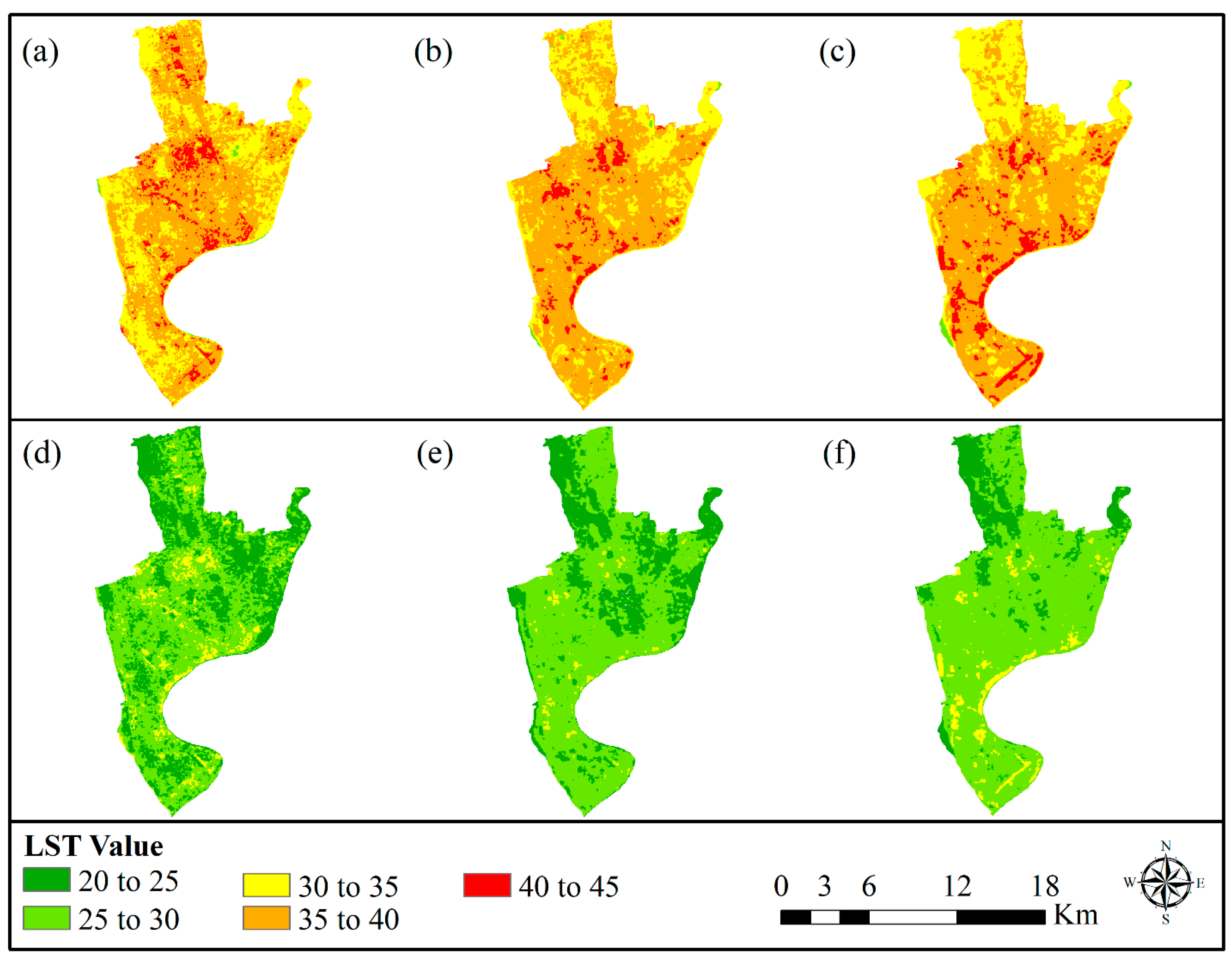
LST analysis reveals a clear progression of thermal intensification across CCC. The spatial patterns for both seasons are shown in Figure 10, and the distribution of temperature ranges is summarized in

Table 7. Percentage distribution of LST ranges across study years and seasons in CCC.

LST (°C)	2004		2014		2024
	S	W	S	W	S	W
20–25	0.00	46.73	0.00	28.83	0.00	15.89
25–30	0.61	50.58	0.51	69.48	0.47	78.64
30–35	33.32	2.62	26.85	1.69	27.37	5.47
35–40	57.99	0.00	66.46	0.00	62.19	0.00
40–45	7.99	0.00	6.18	0.00	9.96	0.00

. High-temperature zones were initially concentrated in the central urban core in 2004. Over time, they expanded toward the periphery along corridors of rapid development.

The LST distributions indicate progressive warming across the study period, particularly during winter. High-temperature zones expanded spatially with ongoing urban development, while cooler temperature classes became progressively less extensive (Table 7). Mean LST increased in both seasons, although warming was substantially stronger during winter. The relatively small summer increase remained within the Landsat retrieval uncertainty and is, therefore, interpreted cautiously (Section 2.7). Winter warming was more pronounced, with a mean increase of 1.72 °C that exceeded the retrieval uncertainty and provides firmer evidence of cool-season thermal intensification.

3.4. Findings from the MODIS–Landsat LST Cross-Comparison

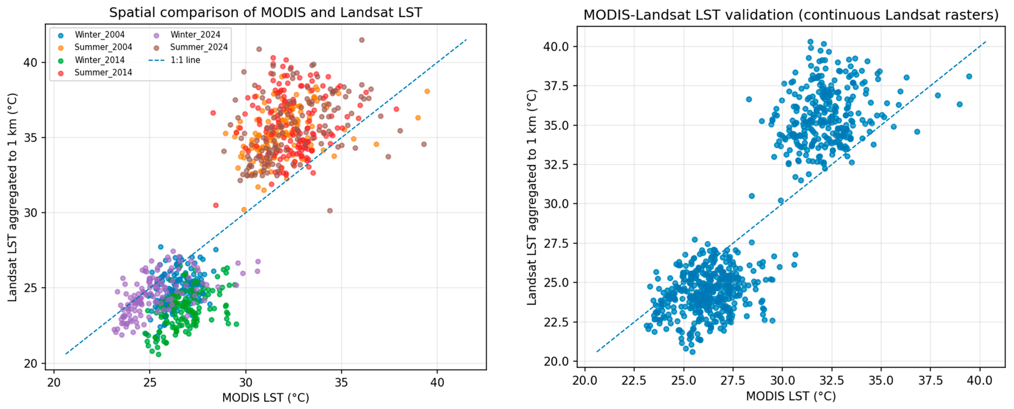
The cross-comparison with the MODIS MOD11A2 product evaluated the spatial consistency of the Landsat-derived LST rather than its absolute accuracy. As summarized in

Table 8. Spatial cross-comparison of Landsat-derived LST against MODIS LST.

Season-Year	Landsat Mean LST (°C)	MODIS Mean LST (°C)	Bias (°C)	MAE (°C)	RMSE (°C)	R2
Winter 2004	27.12	26.50	+0.62	2.31	2.78	0.83
Summer 2004	34.85	32.09	+2.76	3.12	3.65	0.79
Winter 2014	27.90	26.95	+0.95	2.48	2.96	0.85
Summer 2014	35.40	32.62	+2.78	3.05	3.58	0.80
Winter 2024	26.02	25.30	+0.72	2.21	2.69	0.84
Summer 2024	34.10	32.63	+1.47	2.50	3.05	0.75

and Figure 11, the comparison showed good agreement overall (R² = 0.81, RMSE = 3.12 °C), with performance metrics falling within the range commonly reported for Landsat LST retrievals in tropical environments. Landsat consistently produced slightly higher temperatures than MODIS, primarily because of differences in spatial resolution, overpass timing, emissivity treatment, and temporal compositing. These results support the spatial consistency of the Landsat-derived LST while not constituting ground-based validation.

3.5. Relationship Between LULC and LST

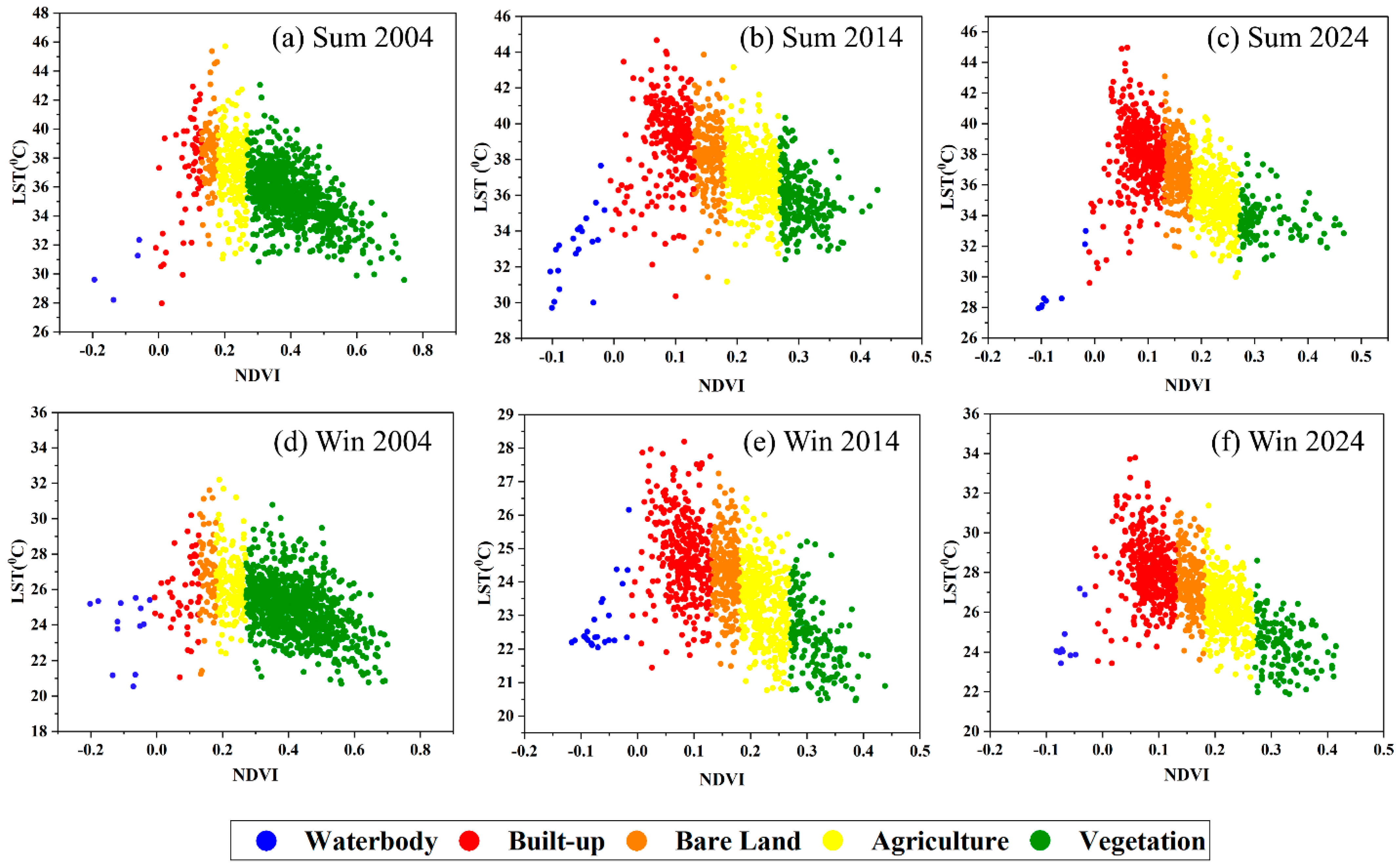
To evaluate the influence of land cover on surface thermal conditions, LST was extracted from 1125 randomly distributed sampling points and grouped according to the NDVI-based land-cover classes defined in Table 3. The distributions are presented in Figure 12, and the corresponding class means are summarized in

Table 9. Derived average LST in different LULC types (°C).

	Year	Agriculture	Bare Land	Built-up	Vegetation	Water Body
Summer	2004	36.55	36.32	37.24	34.81	30.99
	2014	36.17	36.25	37.96	35.08	33.66
	2024	35.97	36.89	38.04	34.74	32.80
Winter	2004	25.85	25.80	26.14	23.95	23.60
	2014	26.22	27.68	26.83	24.45	24.25
	2024	27.30	27.02	27.89	24.88	24.55

. Built-up areas consistently exhibited the highest LST, whereas vegetation and water bodies remained the coolest land-cover classes, highlighting the strong influence of land-cover characteristics on urban thermal behavior.

Built-up areas exhibited substantially stronger warming during winter than summer, indicating a clear seasonal asymmetry in the thermal response of impervious surfaces. Bare land generally recorded the second-highest temperatures, reflecting sparse vegetation cover and limited evaporative cooling, whereas vegetation and water bodies consistently moderated surface temperatures through shading, evapotranspiration, and high heat capacity [38,39,40,41,42,43,44,45]. The thermal contrast between built-up areas and natural land-cover classes increased over the study period, indicating progressive intensification of the urban thermal environment as urban expansion continued. The physical mechanisms underlying these seasonal differences are explored further through the controlled statistical analyses in Section 3.7, and discussed in Section 4.2.

3.6. Regression Analysis Between Land Use Indices and LST

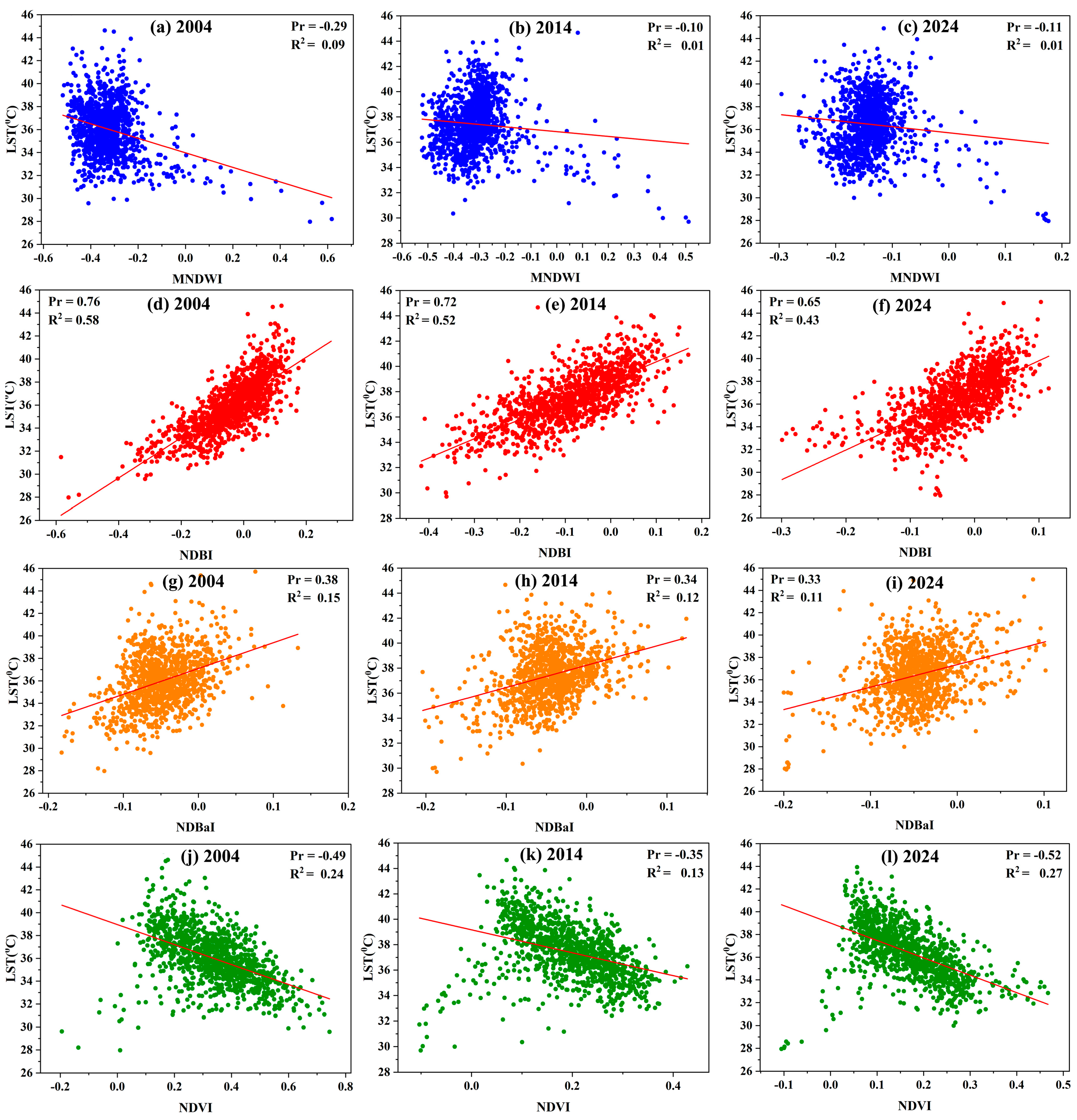
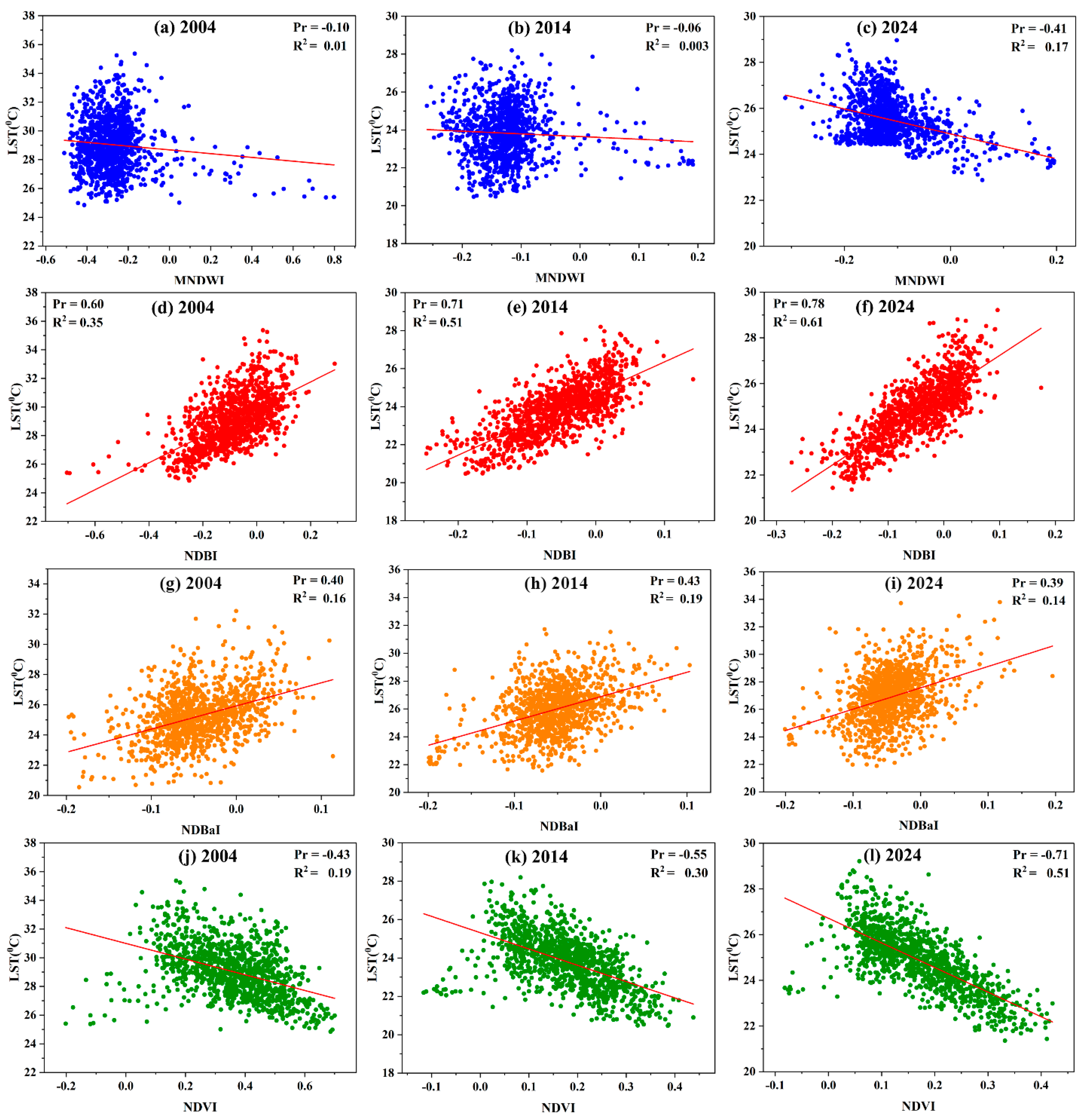
The bivariate relationships between each spectral index and LST are presented in Figure 13 and Figure 14 for the summer and winter seasons. NDBI consistently exhibited the strongest positive association with LST across all years, confirming the dominant influence of impervious surfaces on urban warming. NDBaI showed moderate positive correlations, with stronger relationships during summer than in winter, indicating a greater contribution of bare surfaces to thermal variability under high summer radiation. In contrast, NDVI maintained a consistent negative correlation with LST, reflecting the cooling effects of vegetation, whereas MNDWI exhibited comparatively weaker negative correlations. The evolving MNDWI–LST relationship and the contrasting seasonal trends in water bodies are examined further using the controlled statistical analyses in Section 3.7.

3.7. Controlled Correlation and Regression Analysis

To account for potential confounding effects, the bivariate analyses were extended using partial correlation and multiple regression while controlling for elevation, distance to water, population density, season, and year. As summarized in

Table 10. Partial correlation between LST and environmental variables after controlling for season, year, elevation, distance to water, population density, and other spectral indices.

Variable	Partial r	95% CI	p-Value	Interpretation
NDVI	−0.111	−0.135 to −0.087	<0.001	Independent vegetation cooling
NDBI	0.307	0.285 to 0.329	<0.001	Strongest warming factor
MNDWI	−0.067	−0.091 to −0.043	<0.001	Water/moisture reduces LST
NDBaI	0.097	0.073 to 0.121	<0.001	Bare land warming

, the principal relationships remained significant after adjustment. NDBI retained the strongest positive association with LST, confirming impervious surface intensity as the dominant driver of urban warming. In contrast, NDVI maintained a significant negative relationship, demonstrating that the cooling influence of vegetation is independent of seasonal and spatial covariation. MNDWI and NDBaI also remained significant, although their associations with LST were comparatively weaker.

The multiple regression model explained 64.8% of the observed variation in LST (

Table 11. Multiple regression results explaining LST variability with spectral indices and spatial–temporal control variables (R² = 0.648).

Variable	Coefficient	95% CI	p-Value
NDVI	−0.108	−0.133 to −0.082	<0.001
NDBI	0.228	0.209 to 0.246	<0.001
MNDWI	−0.057	−0.079 to −0.035	<0.001
NDBaI	0.099	0.071 to 0.126	<0.001
Elevation	−0.005	−0.007 to −0.004	<0.001
Distance to water	−0.005	−0.006 to −0.004	<0.001
Population density	2.89 × 10−7	2.03 × 10−7 to 3.75 × 10−7	<0.001

). NDBI emerged as the strongest positive predictor, whereas NDVI, MNDWI, elevation, and distance to water contributed significant negative effects. Population density exhibited a small but significant positive contribution, indicating that densely developed urban areas increase surface temperatures beyond what is captured by the spectral indices alone. Collectively, these results demonstrate that LST variation in Chattogram is governed by the combined effects of land cover, topography, hydrology, urban development, and seasonal variability rather than by any single environmental factor.

The comparatively weak, but increasingly negative, MNDWI–LST relationship should be interpreted within the hydrological context of Chattogram. The city’s heterogeneous water bodies including the Karnaphuli River, estuarine reaches, canals, ponds, and seasonally inundated areas exhibit contrasting thermal characteristics [44]. Consequently, the strengthening negative association over time likely reflects the increasing thermal contrast between the remaining water bodies and the expanding built-up landscape, rather than a change in the intrinsic cooling capacity of water itself [45].

3.8. Statistical Significance of Observed Trends

To assess whether the observed changes exceeded classification and retrieval uncertainty, mean difference tests with 95% confidence intervals were performed for seasonal LST and LULC changes between 2004 and 2024 (

Table 12. Mean LST changes (2004–2024) with 95% confidence intervals and significance tests.

Season	Mean			Changes	CI 95 Changes		p-Value
	2004	2014	2024	2004_2024 (°C)	Low	High
Summer	36.08	36.39	36.50	0.42	0.39	0.43	<0.001
Winter	25.25	25.98	26.97	1.72	1.70	1.74	<0.001

and

Table 13. LULC area changes (2004–2024) with 95% confidence intervals and significance testing.

Class	Season	Δ (%)	Δ (km2)	95% CI (%)	p-Value
Agriculture	Summer	−14.21	−24.11	−14.50 to −13.92	<0.001
Agriculture	Winter	−9.46	−16.05	−9.76 to −9.16	<0.001
Built-up	Summer	+16.33	+27.71	+16.04 to +16.62	<0.001
Built-up	Winter	+17.08	+28.98	+16.79 to +17.37	<0.001
Vegetation	Summer	−6.11	−10.37	−6.39 to −5.83	<0.001
Vegetation	Winter	−5.86	−9.94	−6.14 to −5.58	<0.001
Bare Land	Summer	+3.29	+5.58	+3.11 to +3.47	<0.001
Bare Land	Winter	+0.09	+0.15	−0.05 to +0.23	0.219
Water	Summer	+0.70	+1.19	+0.63 to +0.77	<0.001
Water	Winter	−1.85	−3.14	−1.95 to −1.75	<0.001

).

Winter LST increased by 1.72 °C, exceeding the expected Landsat retrieval uncertainty and providing strong evidence of long-term cool-season warming. In contrast, although the summer increase was statistically significant, its magnitude remained within the expected retrieval uncertainty and should, therefore, be interpreted cautiously. These findings indicate that the winter warming trend is substantially more robust than the corresponding summer trend.

The LULC changes were similarly robust. Built-up area expanded significantly in both seasons, while agriculture and vegetation declined significantly throughout the study period (Table 13). The only non-significant change was winter bare land, consistent with its transitional nature between vegetated and developed land cover classes. Overall, these statistical tests confirm that the observed urban expansion represents a genuine long-term transformation of the landscape and that the associated winter warming cannot be explained solely by classification or retrieval uncertainty.

4. Discussion

4.1. Urban Expansion as the Dominant Driver of Seasonal Surface Warming

Urban expansion has fundamentally reshaped the surface energy balance of Chattogram over the past two decades. The dominance of agricultural-to-built-up conversion observed in the transition matrix indicates that recent urban growth occurred primarily through the outward expansion of the urban footprint. By replacing permeable and vegetated land with impervious surfaces, this transformation reduced evapotranspiration and latent heat exchange, while increasing sensible heat storage, thereby intensifying surface thermal conditions.

The controlled statistical analyses further indicate that the observed thermal changes are primarily driven by land-cover transformation rather than broader environmental variability. The persistence of NDBI as the strongest predictor of LST, together with the robust negative relationship between NDVI and LST after controlling for confounding factors, confirms that the replacement of vegetated landscapes with impervious surfaces is the principal mechanism underlying long-term urban warming in Chattogram. Similar relationships between urban expansion, vegetation loss, and increasing LST have been widely reported in rapidly urbanizing cities worldwide such as Dhaka, Shanghai, and Delhi [41,46,47,48]. However, the present study extends this understanding by demonstrating that the thermal response to urbanization is strongly season-dependent in a tropical coastal environment.

4.2. Seasonal Asymmetry in Urban Warming

A key contribution of this study is the demonstration that the thermal impacts of urbanization are seasonally asymmetric rather than uniform throughout the year. Although summer temperatures remained higher in absolute terms, the greater winter warming indicates that urbanization is altering the seasonal surface energy balance rather than simply increasing temperatures across all seasons. The robust winter warming trend, compared with the relatively modest summer increase, further suggests that continued land-cover transformation has modified both the magnitude and seasonal expression of surface warming in Chattogram.

The stronger winter warming can be explained by seasonal differences in surface energy partitioning. During summer, higher atmospheric moisture, stronger convective mixing, and the moderating influence of the Bay of Bengal limit the additional warming associated with expanding impervious surfaces [5,38,39]. Residual evapotranspiration from the remaining vegetation also offsets heat accumulation through latent heat exchange. During winter, atmospheric moisture is lower, convective activity is weaker, and evapotranspiration is reduced. As a result, surface temperatures become more sensitive to land-cover change [49,50]. Impervious surfaces absorb and retain more heat than surrounding vegetated areas, leading to greater winter warming [40,41]. Similar dry-season amplification of urban warming has been reported in other Bangladeshi cities [42,43].

These findings have broader implications for the assessment of urban climate change. Many LULC–LST studies rely on annual averages or imagery from a single season, implicitly assuming that the effects of urbanization remain constant throughout the year. The present study shows that this assumption can overlook important seasonal differences in urban thermal behavior. This is particularly relevant in tropical coastal environments, where land cover, regional climate, and maritime influences interact differently across seasons [51]. Incorporating seasonal analyses into LULC–LST assessments therefore provides a more complete understanding of urban thermal dynamics and supports more effective climate adaptation and urban planning strategies.

4.3. The Cooling Role of Vegetation and Water Bodies

Beyond the warming effects of urban expansion, the findings highlight the important role of vegetation and water bodies in moderating surface temperatures. NDVI retained a significant negative association with LST in both the bivariate and controlled analyses, indicating that the cooling influence of vegetation remained robust even after controlling for topographic, hydrological, demographic, and seasonal factors. This result reinforces the well-established role of vegetation in regulating urban thermal environments through evapotranspiration, canopy shading, and enhanced latent heat exchange, all of which reduce surface heat accumulation [39,40,41,42,43].

Water bodies also exhibited a consistent cooling effect, although the relationship with LST was weaker than that of vegetation. The controlled analyses suggest that the thermal influence of water is spatially heterogeneous, reflecting differences among the Karnaphuli River, estuarine reaches, urban canals, ponds, and seasonally inundated areas within Chattogram [44]. The increasingly negative MNDWI–LST relationship observed over time likely reflects the growing thermal contrast between the remaining water bodies and the expanding built-up landscape, rather than an increase in the intrinsic cooling capacity of water itself [45]. These findings indicate that conserving urban vegetation and maintaining connected blue–green infrastructure can help moderate local thermal conditions as urbanization continues [52,53].

4.4. Regional Context and Comparative Interpretation

The thermal response observed in Chattogram reflects the influence of its distinctive coastal and topographic setting. Unlike inland South Asian cities such as Dhaka or Delhi, where continental climatic conditions generally promote stronger summer heat accumulation, Chattogram is influenced by maritime air masses from the Bay of Bengal and a complex landscape of coastal plains and surrounding hills [15,16,17]. These geographical characteristics modify the local surface energy balance, resulting in a thermal response that differs from that reported for many inland urban environments.

The findings also demonstrate that comparisons of urban warming across cities should be interpreted with caution. Although studies from Dhaka, Rajshahi, and Mymensingh have reported larger increases in LST, direct numerical comparisons are constrained by differences in observation periods, image selection, retrieval algorithms, emissivity corrections, and analytical approaches. Rather than focusing solely on the magnitude of warming, the present study highlights the importance of considering local geographical and climatic conditions when interpreting urban thermal trends. The pronounced winter warming observed in Chattogram suggests that coastal tropical cities may exhibit seasonally distinct responses to urbanization that are not fully captured by studies based on annual averages or single-season observations.

4.5. Implications for Urban Planning

The findings of this study provide practical guidance for climate-responsive urban planning in rapidly urbanizing tropical coastal cities. The strong association between impervious surface expansion and increasing LST indicates that future development should prioritize compact, climate-sensitive growth while limiting unnecessary surface sealing. Preserving existing vegetation, urban open spaces, and ecologically important wetlands should be a central component of land-use planning. Expanding urban forests, street trees, parks, green roofs, and other forms of green infrastructure can reduce surface temperatures through shading and evapotranspiration, while also improving biodiversity, air quality, and human thermal comfort.

The findings also underscore the importance of strengthening blue infrastructure as part of an integrated urban climate adaptation strategy. Conserving and restoring rivers, canals, ponds, and other urban water bodies, including degraded waterways such as Mahesh Khal, can enhance local cooling, improve stormwater conveyance, restore ecological connectivity, and reduce flooding and waterlogging risks in this low-lying coastal city [54,55]. Rather than functioning as isolated landscape elements, blue and green infrastructure should be planned as interconnected networks that deliver multiple ecosystem services while enhancing resilience to urbanization and climate change.

The pronounced seasonal differences identified in this study further indicate that urban climate planning should account for seasonal variability rather than relying solely on annual averages or single-season observations. A seasonally informed planning approach can better identify periods and locations of elevated thermal exposure, enabling more targeted mitigation measures and more efficient allocation of urban resources. Integrating seasonal thermal analyses into land-use planning, urban greening programs, and climate adaptation policies would therefore strengthen the resilience of Chattogram and other rapidly developing tropical coastal cities facing similar challenges.

4.6. Limitations and Future Research

A major strength of this study is the integration of multi-season Landsat observations, spectral indices, LULC transition analysis, and controlled statistical modeling within a unified analytical framework. By combining seasonal compositing with partial correlation and multiple regression, the study provides a more comprehensive assessment of urban thermal dynamics than conventional analyses based on annual observations or simple bivariate relationships. The independent cross-comparison with MODIS further supports the spatial consistency of the Landsat-derived LST.

Several limitations should nevertheless be acknowledged. The analysis is based on three representative observation years spanning two decades and therefore cannot fully capture interannual climatic variability. In addition, the 30 m spatial resolution of Landsat may introduce mixed-pixel effects in heterogeneous urban environments, while important factors such as building height, urban morphology, anthropogenic heat emissions, and traffic were not explicitly incorporated into the statistical models [56,57]. Furthermore, LST represents surface thermal conditions rather than near-surface air temperature experienced by residents, and continuous ground-based observations were unavailable to provide direct validation of the satellite-derived estimates. Consequently, the relatively small summer warming trend should be interpreted with appropriate caution.

Although a complementary analysis using the Temperature Vegetation Dryness Index (TVDI) produced results consistent with the observed patterns of urban warming, it was not included in the primary analysis because its formulation combines LST and NDVI, preventing an independent assessment of their respective contributions. Moreover, the estimation of TVDI dry and wet edges is less reliable in humid, topographically complex coastal environments [58,59,60]. Future research may further explore TVDI for drought and soil moisture applications. (Table S3) (Figures S1 and S2).

Future research should extend the temporal record using additional observation years and higher-resolution thermal datasets. As tropical coastal cities continue to expand under a changing climate, incorporating seasonal thermal dynamics into land-use planning will be essential for developing more resilient and sustainable urban environments.

5. Conclusions

This study examined the influence of long-term LULC transformation on seasonal LST dynamics in CCC over 2004–2024, using multi-temporal Landsat imagery, spectral indices, and controlled statistical analysis. Rapid urban expansion has substantially altered the city’s surface characteristics. Agricultural land and vegetation have been converted into impervious built-up areas, measurably modifying the urban thermal environment.

The central contribution of this work is the finding that urban warming in this tropical coastal city is seasonally asymmetric rather than uniform. Winter showed a statistically significant warming trend. The smaller summer increase, by contrast, remained within the uncertainty range of Landsat-derived surface temperature. Warming has therefore intensified more strongly during the cooler season, narrowing the seasonal thermal contrast. Built-up intensity emerged as the dominant driver of this warming, while vegetation consistently lowered LST. This underlines the role of natural land cover in regulating urban thermal conditions.

These results carry direct implications for planning and climate adaptation. Preserving vegetation, protecting urban water bodies, and integrating green infrastructure into future development can help moderate surface temperatures as Chattogram expands. The analytical framework applied here can also be transferred to other rapidly urbanizing tropical coastal cities facing similar development challenges. More broadly, the study shows that seasonal differences are essential to understanding how urbanization influences surface temperature. Seasonal warming should, therefore, be considered explicitly in future urban climate assessments, rather than obscured within annual averages.

References

1. United Nations, Department of Economic and Social Affairs, Population Division. World Urbanization Prospects: The 2018 Revision; United Nations: New York, NY, USA, 2018; Available online: https://population.un.org/wup (accessed on 20 January 2025).
2. Kafy, A.A.; Faisal, A.A.; Rahman, M.S.; Islam, M.; Rakib, A.A.; Islam, M.A.; Khan, M.H.H.; Sikdar, M.S.; Sarker, M.H.S.; Mawa, J.; et al. Prediction of seasonal urban thermal field variance index using machine learning algorithms in Cumilla, Bangladesh. Sustain. Cities Soc. 2021, 64, 102542. [Google Scholar] [CrossRef]
3. Oke, T.R.; Mills, G.; Christen, A.; Voogt, J.A. Urban Climates; Cambridge University Press: Cambridge, UK, 2017. [Google Scholar] [CrossRef]
4. Kafy, A.A.; Rahman, M.S.; Faisal, A.; Hasan, M.M.; Islam, M. Modelling future land use land cover changes and their impacts on land surface temperatures in Rajshahi, Bangladesh. Remote Sens. Appl. Soc. Environ. 2020, 18, 100314. [Google Scholar] [CrossRef]
5. Arnfield, A.J. Two decades of urban climate research: A review of turbulence, exchanges of energy and water, and the urban heat island. Int. J. Climatol. 2003, 23, 1–26. [Google Scholar] [CrossRef]
6. Huang, X.; Wang, Y.; Li, J.; Chang, X.; Cao, Y.; Xie, J. High-resolution urban land-cover mapping and landscape analysis of the 42 major cities in China using ZY-3 satellite images. Sci. Bull. 2020, 65, 1039–1048. [Google Scholar] [CrossRef] [PubMed]
7. Rinner, C.; Hussain, M. Toronto’s urban heat island—Exploring the relationship between land use and surface temperature. Remote Sens. 2011, 3, 1251–1265. [Google Scholar] [CrossRef]
8. Yang, C.; He, X.; Yan, F.; Yu, L.; Bu, K.; Yang, J.; Chang, L.; Zhang, S. Mapping the influence of land use/land cover changes on the urban heat island effect—A case study of Changchun, China. Sustainability 2017, 9, 312. [Google Scholar] [CrossRef]
9. Chaudhuri, G.; Mishra, N.B. Spatio-temporal dynamics of land cover and land surface temperature in Ganges-Brahmaputra delta: A comparative analysis between India and Bangladesh. Appl. Geogr. 2016, 68, 68–83. [Google Scholar] [CrossRef]
10. Rashid, N.; Alam, J.A.M.M.; Chowdhury, M.A.; Islam, S.L.U. Impact of landuse change and urbanization on urban heat island effect in Narayanganj city, Bangladesh: A remote sensing-based estimation. Environ. Chall. 2022, 8, 100571. [Google Scholar] [CrossRef]
11. Mohammad, P.; Goswami, A.; Bonafoni, S. The impact of the land cover dynamics on surface urban heat island variations in semi-arid cities: A case study in Ahmedabad City, India, using multi-sensor/source data. Sensors 2019, 19, 3701. [Google Scholar] [CrossRef] [PubMed]
12. Hua, A.K.; Ping, O.W. The influence of land-use/land-cover changes on land surface temperature: A case study of Kuala Lumpur metropolitan city. Eur. J. Remote Sens. 2018, 51, 1049–1069. [Google Scholar] [CrossRef]
13. Aik, D.H.B.; Ismail, M.H.; Muharam, F.M. Land use/land cover changes and the relationship with land surface temperature using Landsat and MODIS imageries in Cameron Highlands, Malaysia. Land 2020, 9, 372. [Google Scholar] [CrossRef]
14. Sresto, M.A.; Siddika, S.; Fattah, M.A.; Morshed, S.R.; Morshed, M.M. A GIS and remote sensing approach for measuring summer-winter variation of land use and land cover indices and surface temperature in Dhaka district, Bangladesh. Heliyon 2022, 8, e10309. [Google Scholar] [CrossRef] [PubMed]
15. Mohan, M.; Kandya, A.; Battiprolu, A. Urban Heat Island Effect over National Capital Region of India: A Study Using the Temperature Trends. J. Environ. Prot. 2011, 2, 465–472. [Google Scholar] [CrossRef]
16. Nath, T.K.; Inoue, M.; Chakma, S. Shifting Cultivation (Jhum) in the Chittagong Hill Tracts, Bangladesh: Examining Its Sustainability, Rural Livelihood and Policy Implications. Int. J. Agric. Sustain. 2005, 3, 130–142. [Google Scholar] [CrossRef]
17. Shahid, S. Recent Trends in the Climate of Bangladesh. Clim. Res. 2010, 42, 185–193. [Google Scholar] [CrossRef]
18. Shahriar, S.A.; Kayes, I.; Hasan, K.; Hasan, M.; Islam, R.; Awang, N.R.; Hamzah, Z. Potential of ARIMA-ANN, ARIMA-SVM, DT and CatBoost for atmospheric PM2.5 forecasting in Bangladesh. Atmosphere 2021, 12, 100. [Google Scholar] [CrossRef]
19. Roy, S.; Pandit, S.; Eva, E.A.; Bagmar, M.S.H.; Papia, M.; Banik, L.; Dube, T.; Rahman, F.; Razi, M.A. Examining the nexus between land surface temperature and urban growth in Chattogram Metropolitan Area of Bangladesh using long term Landsat series data. Urban Clim. 2020, 32, 100593. [Google Scholar] [CrossRef]
20. Huraira, A.; Jui, T.J.; Samm, A.A.; Samad, N.; Sarker, S. Spatial Trend Analysis of Atmospheric Pollutants in Chattogram District of Bangladesh Using Sentinel-5 TROPOMI Images. Dhaka Univ. J. Earth Environ. Sci. 2024, 13, 105–123. [Google Scholar] [CrossRef]
21. Biswas, J.; Jobaer, M.A.; Haque, S.F.; Islam Shozib, M.S.; Limon, Z.A. Mapping and Monitoring Land Use Land Cover Dynamics Employing Google Earth Engine and Machine Learning Algorithms on Chattogram, Bangladesh. Heliyon 2023, 9, e21245. [Google Scholar] [CrossRef] [PubMed]
22. U.S. Geological Survey. Landsat 8–9 Collection 2 Level 2 Science Product Guide, Version 6.0; U.S. Geological Survey, Earth Resources Observation and Science (EROS) Center: Sioux Falls, SD, USA, 2024. Available online: https://www.usgs.gov/landsat-missions/landsat-collection-2-level-2-science-products (accessed on 10 December 2025).
23. U.S. Geological Survey. Landsat 4–7 Collection 2 Level-2 Science Product Guide; U.S. Geological Survey: Sioux Falls, SD, USA. Available online: https://www.usgs.gov/media/files/landsat-4-7-collection-2-level-2-science-product-guide?utm_source=chatgpt.com (accessed on 20 November 2025).
24. Grigoraș, G.; Urițescu, B. Land use/land cover changes dynamics and their effects on surface urban heat island in Bucharest, Romania. Int. J. Appl. Earth Obs. Geoinf. 2019, 80, 115–126. [Google Scholar] [CrossRef]
25. Breiman, L. Random Forests. Mach. Learn. 2001, 45, 5–32. [Google Scholar] [CrossRef]
26. Belgiu, M.; Drăguţ, L. Random Forest in Remote Sensing: A Review of Applications and Future Directions. ISPRS J. Photogramm. Remote Sens. 2016, 114, 24–31. [Google Scholar] [CrossRef]
27. Tucker, C.J. Red and photographic infrared linear combinations for monitoring vegetation. Remote Sens. Environ. 1979, 8, 127–150. [Google Scholar] [CrossRef]
28. Zha, Y.; Gao, J.; Ni, S. Use of normalized difference built-up index in automatically mapping urban areas from TM imagery. Int. J. Remote Sens. 2003, 24, 583–594. [Google Scholar] [CrossRef]
29. Zhao, H.; Chen, X. Use of normalized difference bareness index in quickly mapping bare areas from TM/ETM+. In Proceedings of the IEEE International Geoscience and Remote Sensing Symposium (IGARSS), Seoul, Republic of Korea, 29–29 July 2005; Volume 3, pp. 1666–1668. [Google Scholar] [CrossRef]
30. Xu, H. Modification of normalised difference water index (NDWI) to enhance open water features in remotely sensed imagery. Int. J. Remote Sens. 2006, 27, 3025–3033. [Google Scholar] [CrossRef]
31. Taharchaouche, I. Detection of land use/land cover change and land surface temperature in the eastern part of Batna City (North East Algeria) using remote sensing data and GIS. J. Geol. Geogr. Geoecol. 2023, 32, 632–643. [Google Scholar] [CrossRef] [PubMed]
32. Akbar, T.A.; Hassan, Q.K.; Ishaq, S.; Batool, M.; Butt, H.J.; Jabbar, H. Investigative spatial distribution and modelling of existing and future urban land changes and its impact on urbanization and economy. Remote Sens. 2019, 11, 105. [Google Scholar] [CrossRef]
33. Laraby, K.G.; Schott, J.R. Uncertainty Estimation Method and Landsat 7 Global Validation for the Landsat Surface Temperature Product. Remote Sens. Environ. 2018, 216, 472–481. [Google Scholar] [CrossRef]
34. U.S. Geological Survey. MODIS/Terra Land Surface Temperature/Emissivity 8-Day L3 Global 1 km SIN Grid, MOD11A2, Version 6.1; NASA LP DAAC: Sioux Falls, SD, USA, 2021. Available online: https://ladsweb.modaps.eosdis.nasa.gov/missions-and-measurements/products/MOD11A2?utm (accessed on 10 February 2026).
35. Duan, S.-B.; Li, Z.-L.; Li, H.; Göttsche, F.-M.; Wu, H.; Zhao, W.; Leng, P.; Zhang, X.; Coll, C. Validation of Landsat Land Surface Temperature Product in the Conterminous United States Using In Situ Measurements from SURFRAD, ARM, and NDBC Sites. Int. J. Digit. Earth 2021, 14, 640–660. [Google Scholar] [CrossRef]
36. Zhong, C.; Peng, L.; Yu, J.; Swan, I.; Li, H. Toward More Reliable, Complete, and Equitable Global Urban Land Use Efficiency Assessments. Commun. Earth Environ. 2025, 6, 1055. [Google Scholar] [CrossRef]
37. Sen, P.K. Estimates of the regression coefficient based on Kendall’s tau. J. Am. Stat. Assoc. 1968, 63, 1379–1389. [Google Scholar] [CrossRef]
38. Oke, T.R. The energetic basis of the urban heat island. Q. J. R. Meteorol. Soc. 1982, 108, 1–24. [Google Scholar] [CrossRef]
39. Peng, S.; Piao, S.; Ciais, P.; Friedlingstein, P.; Ottle, C.; Bréon, F.-M.; Nan, H.; Zhou, L.; Myneni, R.B. Surface urban heat island across 419 global big cities. Environ. Sci. Technol. 2012, 46, 696–703. [Google Scholar] [CrossRef] [PubMed]
40. Imhoff, M.L.; Zhang, P.; Wolfe, R.E.; Bounoua, L. Remote sensing of the urban heat island effect across biomes in the continental USA. Remote Sens. Environ. 2010, 114, 504–513. [Google Scholar] [CrossRef]
41. Zhao, L.; Lee, X.; Smith, R.B.; Oleson, K. Strong contributions of local background climate to urban heat islands. Nature 2014, 511, 216–219. [Google Scholar] [CrossRef] [PubMed]
42. Dewan, A.M.; Kabir, M.H.; Nahar, K.; Rahman, M.Z. Urbanisation and environmental degradation in Dhaka Metropolitan Area of Bangladesh. Int. J. Environ. Sustain. Dev. 2012, 11, 118. [Google Scholar] [CrossRef]
43. Rahman, S.; Touhiduzzaman, M.; Hasan, I. Coastal livelihood vulnerability to climate change: A case study of Char Montaz in Patuakhali District of Bangladesh. Am. J. Mod. Energy 2017, 3, 58. [Google Scholar] [CrossRef][Green Version]
44. Sun, R.; Chen, A.; Chen, L.; Lü, Y. Cooling Effects of Wetlands in an Urban Region: The Case of Beijing. Ecol. Indic. 2012, 20, 57–64. [Google Scholar] [CrossRef]
45. Hathway, E.A.; Sharples, S. The Interaction of Rivers and Urban Form in Mitigating the Urban Heat Island Effect: A UK Case Study. Build. Environ. 2012, 58, 14–22. [Google Scholar] [CrossRef]
46. Weng, Q. Thermal infrared remote sensing for urban climate and environmental studies: Methods, applications, and trends. ISPRS J. Photogramm. Remote Sens. 2009, 64, 335–344. [Google Scholar] [CrossRef]
47. Li, J.; Song, C.; Cao, L.; Zhu, F.; Meng, X.; Wu, J. Impacts of landscape structure on surface urban heat islands: A case study of Shanghai, China. Remote Sens. Environ. 2011, 115, 3249–3263. [Google Scholar] [CrossRef]
48. Singh, R.B.; Grover, A.; Zhan, J. Inter-Seasonal Variations of Surface Temperature in the Urbanized Environment of Delhi Using Landsat Thermal Data. Energies 2014, 7, 1811–1828. [Google Scholar] [CrossRef]
49. Corlett, R.T.; Lafrankie, J.V. Potential Impacts of Climate Change on Tropical Asian Forests through an Influence on Phenology. Clim. Change 1998, 39, 439–453. [Google Scholar] [CrossRef]
50. Numata, S.; Yamaguchi, K.; Shimizu, M.; Sakurai, G.; Morimoto, A.; Alias, N.; Noor Azman, N.Z.; Hosaka, T.; Satake, A. Impacts of Climate Change on Reproductive Phenology in Tropical Rainforests of Southeast Asia. Commun. Biol. 2022, 5, 311. [Google Scholar] [CrossRef] [PubMed]
51. World Bank. An Unsustainable Life: The Impact of Heat on Health and the Economy of Bangladesh; World Bank: Washington, DC, USA, 2025; Available online: https://www.worldbank.org (accessed on 20 January 2026).
52. Wu, S.; Yang, H.; Luo, P.; Luo, C.; Li, H.; Liu, M.; Ruan, Y.; Zhang, S.; Xiang, P.; Jia, H.; et al. The effects of the cooling efficiency of urban wetlands in an inland megacity: A case study of Chengdu, Southwest China. Build. Environ. 2021, 204, 108128. [Google Scholar] [CrossRef]
53. Weng, Q.; Lu, D.; Schubring, J. Estimation of land surface temperature–vegetation abundance relationship for urban heat island studies. Remote Sens. Environ. 2004, 89, 467–483. [Google Scholar] [CrossRef]
54. Islam, M.R.; Raja, D.R. Waterlogging Risk Assessment: An Undervalued Disaster Risk in Coastal Urban Community of Chattogram, Bangladesh. Earth 2021, 2, 151–173. [Google Scholar] [CrossRef]
55. Masum, M.H.; Hossen, J.; Pal, S.K. Hydrologic Performance of Drainage Network under Different Climatic and Land-Use Conditions: A Case Study of Chattogram. J. Soft Comput. Civ. Eng. 2020, 4, 1–23. [Google Scholar] [CrossRef]
56. Santamouris, M. Regulating the damaged thermostat of the cities—Status, impacts and mitigation challenges. Energy Build. 2015, 91, 43–56. [Google Scholar] [CrossRef]
57. Stewart, I.D.; Oke, T.R. Local climate zones for urban temperature studies. Bull. Am. Meteorol. Soc. 2012, 93, 1879–1900. [Google Scholar] [CrossRef]
58. Sandholt, I.; Rasmussen, K.; Andersen, J. A Simple Interpretation of the Surface Temperature/Vegetation Index Space for Assessment of Surface Moisture Status. Remote Sens. Environ. 2002, 79, 213–224. [Google Scholar] [CrossRef]
59. Yuan, Y.; Ye, X.; Liu, T.; Li, X. Drought Monitoring Based on Temperature Vegetation Dryness Index and Its Relationship with Anthropogenic Pressure in a Subtropical Humid Watershed in China. Ecol. Indic. 2023, 154, 110584. [Google Scholar] [CrossRef]
60. Wang, C.; Qi, S.; Niu, Z.; Wang, J. Evaluating Soil Moisture Status in China Using the Temperature–Vegetation Dryness Index (TVDI). Can. J. Remote Sens. 2004, 30, 671–679. [Google Scholar] [CrossRef]
Figure 1. Sequential workflow of the proposed framework.
Geographies 06 00072 g001
Figure 2. Map of the study area of CCC.
Geographies 06 00072 g002
Figure 3. LULC patterns of CCC during the summer season of (a) 2004, (b) 2014, and (c) 2024 and the winter season of (d) 2004, (e) 2014, and (f) 2024.
Geographies 06 00072 g003
Figure 4. LULC transition matrix of CCC in (a) summer and (b) winter during 2004–2024.
Geographies 06 00072 g004
Figure 5. NDBI profile of the study area during the summer season of (a) 2004, (b) 2014, and (c) 2024, and the winter season of (d) 2004, (e) 2014, and (f) 2024.
Geographies 06 00072 g005
Figure 6. NDBaI profile of the study area during the summer season of (a) 2004, (b) 2014, and (c) 2024, and the winter season of (d) 2004, (e) 2014, and (f) 2024.
Geographies 06 00072 g006
Figure 7. MNDWI profile of the study area during the summer season of (a) 2004, (b) 2014, and (c) 2024, and the winter season of (d) 2004, (e) 2014, and (f) 2024.
Geographies 06 00072 g007
Figure 8. NDVI profile of the study area during the summer season of (a) 2004, (b) 2014, and (c) 2024, and the winter season of (d) 2004, (e) 2014, and (f) 2024.
Geographies 06 00072 g008
Figure 9. Min, max, and mean values for NDBI, NDBaI, MNDWI, and NDVI of 2004, 2014, and 2024.
Geographies 06 00072 g009
Figure 10. Derived LST profile of the study area during the summer season of (a) 2004, (b) 2014, and (c) 2024 and the winter season of (d) 2004, (e) 2014, and (f) 2024.
Geographies 06 00072 g010
Figure 11. Spatial cross-comparison of Landsat-derived LST with MODIS LST: (left panel) multi-season scatter plot of all six seasonal cases; (right panel) pixel-level scatter plot of the aggregated Landsat rasters against MODIS LST. The dashed line in each panel represents the 1:1 reference.
Geographies 06 00072 g011
Figure 12. Distributions of LST in different LULC types.
Geographies 06 00072 g012
Figure 13. Correlation between the summer season land use indices and LST during 2004–2024.
Geographies 06 00072 g013
Figure 14. Correlation between the winter season land use indices and LST during 2004–2024.
Geographies 06 00072 g014