Article

Streamflow Simulation in the Cau River Basin, Northeast Vietnam, Using SWAT-Based Hydrological Modelling

1
Faculty of Resource Management, University of Agriculture and Forestry—Thai Nguyen University, Thai Nguyen 250000, Vietnam
2
Faculty of Basic Science, University of Agriculture and Forestry—Thai Nguyen University, Thai Nguyen 250000, Vietnam
3
Mathematics and Geospatial Science, STEM College, RMIT University, Melbourne, VIC 3000, Australia
*
Author to whom correspondence should be addressed.
Geographies 2025, 5(3), 41; https://doi.org/10.3390/geographies5030041
Submission received: 18 June 2025 / Revised: 23 July 2025 / Accepted: 8 August 2025 / Published: 13 August 2025

Abstract

The Cau River Basin in northeastern Vietnam is an ecologically and economically important watershed, yet it has lacked comprehensive hydrological modelling to date. Characterised by highly complex topography, diverse land use/land cover, and limited hydrometeorological data, the basin presents challenges for water resource assessment and management. This study applies the SWAT hydrological model to simulate streamflow dynamics in the Cau River Basin over a 31-year period (1990–2020) using multiple-source geospatial data, including a 30 m digital elevation model, official soil and land use maps, and daily climate records from six meteorological stations. Model calibration (1997–2008) and validation (2009–2020) were conducted using the SWAT-CUP tool, achieving strong performance with a Nash–Sutcliffe Efficiency (NSE) of 0.95 and 0.90, and R2 of 0.95 and 0.91, respectively. Sensitivity analysis identified four key parameters most influential on streamflow (curve number, saturated hydraulic conductivity, soil evaporation compensation factor, and available water capacity), supporting a more focused and effective calibration process. Model results revealed substantial spatio-temporal variability in runoff, with annual surface runoff ranging from 19.8 mm (2011) to 56.4 mm (2013), generally lower in upstream sub-watersheds (<30 mm) and higher in downstream areas (>60 mm). The simulations also showed a clear seasonal contrast between the wet and dry periods. These findings support evidence-based strategies for flood and drought mitigation, inform agricultural and land use planning, and offer a transferable modelling framework for similarly complex watersheds.

1. Introduction

Hydrological modelling has emerged as a fundamental component of contemporary water resource management, particularly as global systems face unprecedented pressures from anthropogenic activities and climate variability [1,2,3]. The intricate relationship between human development and natural hydrological processes has become increasingly complex, with global population growth, rapid industrialization, and evolving land use patterns substantially altering the availability and distribution of freshwater resources [4,5,6,7]. These anthropogenic modifications fundamentally disrupt natural hydrological cycles by influencing critical processes including infiltration rates, groundwater recharge mechanisms, evapotranspiration patterns, and surface runoff generation [2,3,7]. The resulting changes in catchment physiographic characteristics, including surface roughness and vegetation cover dynamics, produce significant impacts on both streamflow volume and temporal distribution patterns [8,9,10,11]. Consequently, accurate streamflow estimation at the catchment scale has become essential for developing sustainable water allocation frameworks and implementing effective management strategies [1,2,3,12,13].
In Southeast Asia, Vietnam exemplifies the complex water resource challenges facing rapidly developing nations in monsoon-dominated regions. The country’s river basins experience mounting pressures from escalating climate change impacts, accelerated urbanization, and intensive agricultural and industrial development [5,6,14]. Among these systems, the Cau River Basin represents a particularly significant case study, covering an area exceeding 6000 km2 across the northern mountainous midland region [15]. This transboundary watershed serves as a critical water source for domestic, agricultural, and industrial purposes while maintaining ecological balance across the provinces of Thai Nguyen, Bac Kan, Bac Giang, and Bac Ninh. However, the basin currently confronts multiple interconnected challenges that threaten its hydrological sustainability [15,16]. These include diminishing dry season streamflow, accelerated slope soil erosion [17], increasing water pollution from agricultural runoff and industrial discharges [18,19,20], and heightened risks of localised flooding during intensive rainfall periods [21]. The complex topography and transboundary nature of the basin compound these challenges by limiting data accessibility and complicating integrated management approaches [7,9,22].
The scientific community has responded to hydrological assessment challenges through the development and application of sophisticated modelling frameworks [23]. Among available approaches, physically-based rainfall–runoff models have demonstrated superior performance in streamflow estimation studies due to their explicit representation of runoff generation mechanisms grounded in fundamental physical principles [2,7,10,24]. These models offer significant advantages over empirical approaches by maintaining physical meaning across different temporal and spatial scales while providing mechanistic insights into hydrological process interactions [1,9]. The Soil and Water Assessment Tool (SWAT) exemplifies the capabilities of such physically-based modelling systems, having established itself as one of the most widely applied semi-distributed hydrological models globally [2]. Originally developed by the United States Department of Agriculture, SWAT has proven particularly valuable for simulating the complex interactions between climatic, topographic, and anthropogenic factors that influence watershed hydrology [22,25,26].
The SWAT model operates using the innovative Hydrologic Response Unit (HRU) concept, wherein the smallest spatial modelling unit aggregates areas with similar soil types, land use/land cover (LULC) classifications, and slope conditions within defined sub-watersheds [10,12,23]. This approach enables detailed representation of spatial heterogeneity while maintaining computational efficiency, making it particularly suitable for large-scale watershed applications [5,7,24]. The model’s comprehensive framework incorporates multiple interconnected components including weather simulation, surface runoff calculation, evapotranspiration estimation, soil water dynamics, groundwater flow modelling, and nutrient cycling processes [25]. This integrated approach has facilitated its successful application across diverse hydrological investigations worldwide, encompassing calibration and sensitivity analyses, uncertainty assessment, LULC and climate change impact studies, non-point source pollution modelling, and best management practice evaluation [2,16,18,24].
Despite the proven capabilities of advanced hydrological models, their implementation in complex terrains such as mountainous regions with limited data availability presents significant methodological challenges. Traditional ground-based data collection approaches often prove inadequate for comprehensive watershed characterisation, particularly in remote or inaccessible areas where detailed physiographic information remains scarce [2,7,9,23,27]. While rainfall monitoring networks can be expanded through strategic gauge installation, acquiring comprehensive spatial data on elevation patterns, slope characteristics, and land use distributions across vast watersheds requires alternative approaches [28,29]. The integration of high-resolution remotely sensed information has proven instrumental in improving hydrological process representation and observational capabilities, representing a critical advancement during an era of increased uncertainty in hydro-climatic projections due to accelerating global environmental change [12,30].
This study employs the SWAT model for simulating streamflow dynamics in the Cau River Basin, northeastern Vietnam, an ecologically and economically vital transboundary watershed that, until now, has lacked comprehensive hydrological modelling. The basin is characterised by complex topography, heterogeneous LULC, and limited hydrometeorological data, posing significant challenges for water resource assessment. This research implements a SWAT modelling framework using multiple-source geospatial inputs to simulate spatio-temporal variations in streamflow across the basin. Key objectives include quantifying water availability at strategic locations, analysing surface runoff and groundwater recharge under varying climatic conditions, and evaluating the impacts of climate variability on hydrological processes.

2. Materials and Methods

2.1. Study Area

The study area is found in the upstream and midstream sections of the Cau River Basin, covering an area of approximately 3300 km2 and spanning the provinces of Bac Kan and Thai Nguyen (Figure 1). The Cau river originates in northwest Bac Kan, flows through the centre of Thai Nguyen province, and eventually merges with the Thai Binh River system [31,32]. The upstream region is characterised by steep, highly dissected mountainous terrain with uneven vegetation cover, resulting in low water retention capacity and high susceptibility to erosion, flash floods, and landslides during the rainy season. In contrast, the midstream and downstream areas, including densely populated urban centres such as Thai Nguyen City, face growing risks of flooding and water pollution due to surface runoff carrying sediment and waste from upstream.
With a humid tropical monsoon climate, the basin receives an average annual rainfall ranging from 1600 to 2400 mm [32], leading to strongly seasonal flow variability. The rainy season (May–October) accounts for about 80% of annual precipitation and often causes large floods and high peak flows, whereas the dry season (November–April) is marked by very low flow volumes [17]. Over the past decades, the Cau River Basin has experienced several major flood events. The 1959, 1968, 1971, 1983, 1986 flood peak at Gia Bay Station served as a reference standard for subsequent years [33]. In 2001, another severe flood occurred, with water levels reaching 28.08 m at the same station. More recently, on September 9, 2024, the flood peak caused by Typhoon Yagi surpassed the 2001 record, reaching 28.81 m. In addition, prolonged heavy rainfall in 2013 and 2017 also resulted in elevated peak flows, posing flood risks and infrastructure damage across the mid- and downstream regions [34]. These events highlight the hydrological sensitivity of the Cau River Basin and underscore the urgent need for hydrological modelling to support water resource planning, flood management, and climate change adaptation in the future.

2.2. Data and Preprocessing

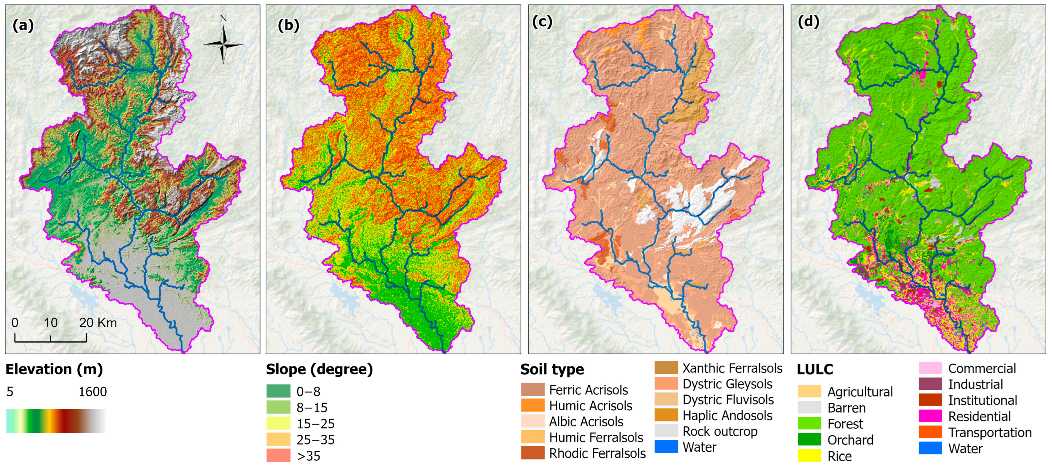
Hydrological modelling through SWAT relies on comprehensive spatial datasets encompassing meteorological parameters at daily intervals, alongside detailed topographic, soil, and LULC data (Figure 2).

2.2.1. Meteorological and Hydrological Data

Meteorological and hydrological inputs are critical for developing, calibrating, and validating the SWAT model. For model development, we used daily precipitation and air temperature (minimum and maximum). Meteorological data spanning 31 years (1990–2020) were collected from six meteorological stations strategically distributed across the study area (Figure 1), effectively capturing the climatic variability of the midland and mountainous regions. All meteorological data were synchronised into a continuous daily time series, checked for logical consistency, and formatted according to SWAT input requirements. For model calibration and validation, observed streamflow data collected at Gia Bay Station (Figure 1) from 1997 to 2020 were used. Using a longer meteorological time series allows for an adequate model warm-up period, which is essential to stabilise soil moisture, groundwater, and other state variables before calibration begins [35,36].

2.2.2. Topographic Data

Topographic information was derived from the Shuttle Radar Topography Mission (SRTM) Digital Elevation Model (DEM), with a spatial resolution of 30 m (Figure 2a). This dataset was freely accessed from the USGS EarthExplorer platform [37,38]. The DEM was utilised to extract stream networks, delineate sub-watersheds, and compute slope (Figure 2b), a key variable for simulating surface runoff and erosion processes [2,25].

2.2.3. Soil Types and Characteristics

Soil data play a fundamental role in the SWAT model, influencing hydrological processes such as infiltration, surface runoff, erosion, and solute transport [2,25,39]. This study utilised 1:100,000 scale soil type maps developed in 2005 by Thai Nguyen and Bac Kan provincial governments. These maps cover the entire Cau River basin (Figure 2c) and are suitable for a semi-distributed modelling approach. To ensure compatibility with SWAT’s database, soil types were standardised using the Food and Agriculture Organisation (FAO) classification system [40] (see Figure 2c for specific soil types). This standardisation enables the use of default soil parameters (e.g., bulk density, saturated hydraulic conductivity, and texture) when field data are limited [35]. Soil parameters, including depth, texture, and saturated hydraulic conductivity (Ksat), were derived from global soil databases, including the Harmonised World Soil Database (HWSD, Version 2.0) [41] and SoilGrids 2.0 [42]. Standardising the soil data also facilitates model application in broader geographic contexts and supports comparative analyses under climate change scenarios.

2.2.4. LULC Data

LULC data represent one of the three key spatial components of the SWAT model, alongside topography and soil. It significantly affects the hydrological behaviour of HRUs, especially in modelling surface runoff, erosion, and sediment or nutrient dynamics [2,35,40]. We used the official 2020 LULC maps developed by the Departments of Natural Resources and Environment of Thai Nguyen and Bac Kan provinces (see Figure 2d). These maps are the most recent and of high accuracy, having been compiled from cadastral records and field surveys. LULC classes were standardised using a code translation table to match the SWAT LULC classification format, ensuring accurate representation of HRU characteristics [35]. The LULC data were integrated into the model via ArcSWAT and formed the basis for simulations of streamflow, sediment yield, and LULC impact assessments on water resources.

2.3. SWAT Model Development

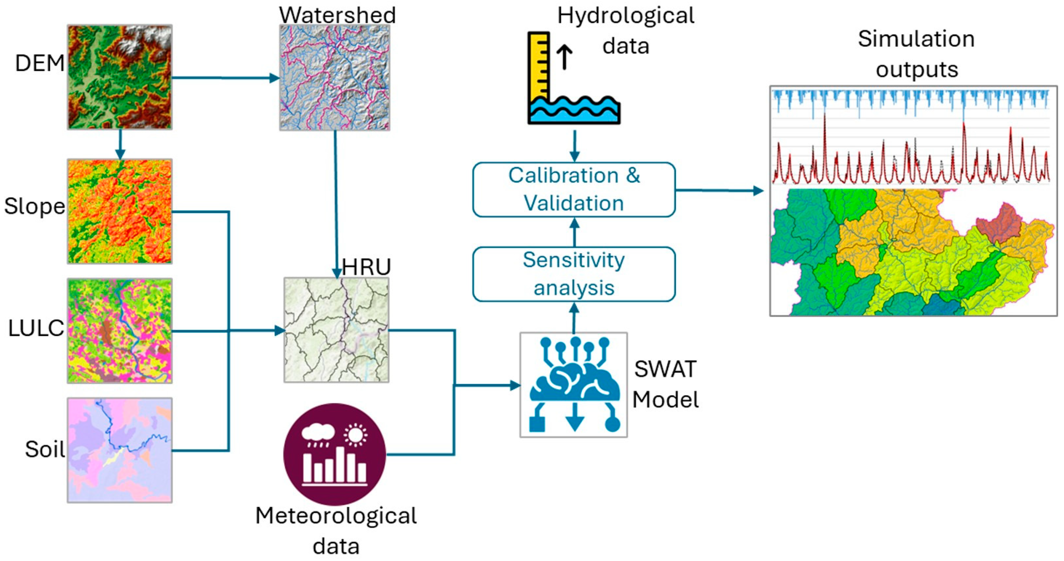
The hydrological modelling in this study was implemented using the SWAT model integrated with ArcGIS (version 10.8) via the ArcSWAT interface (version 2012.10.26). The modelling workflow is illustrated in Figure 3. The first step involved setting up a new SWAT project by specifying the working directory, which contained all necessary spatial and tabular datasets, as well as folders for storing simulation outputs. The next steps were watershed delineation and HRU definition. Dividing the basin into sub-watersheds and HRUs enables the SWAT model to perform simulations within hydrologically homogeneous units, allowing for a more spatially explicit assessment of runoff, the impacts of sediment transport, and LULC or climate change at the regional or sub-basin scale [10,35,40].
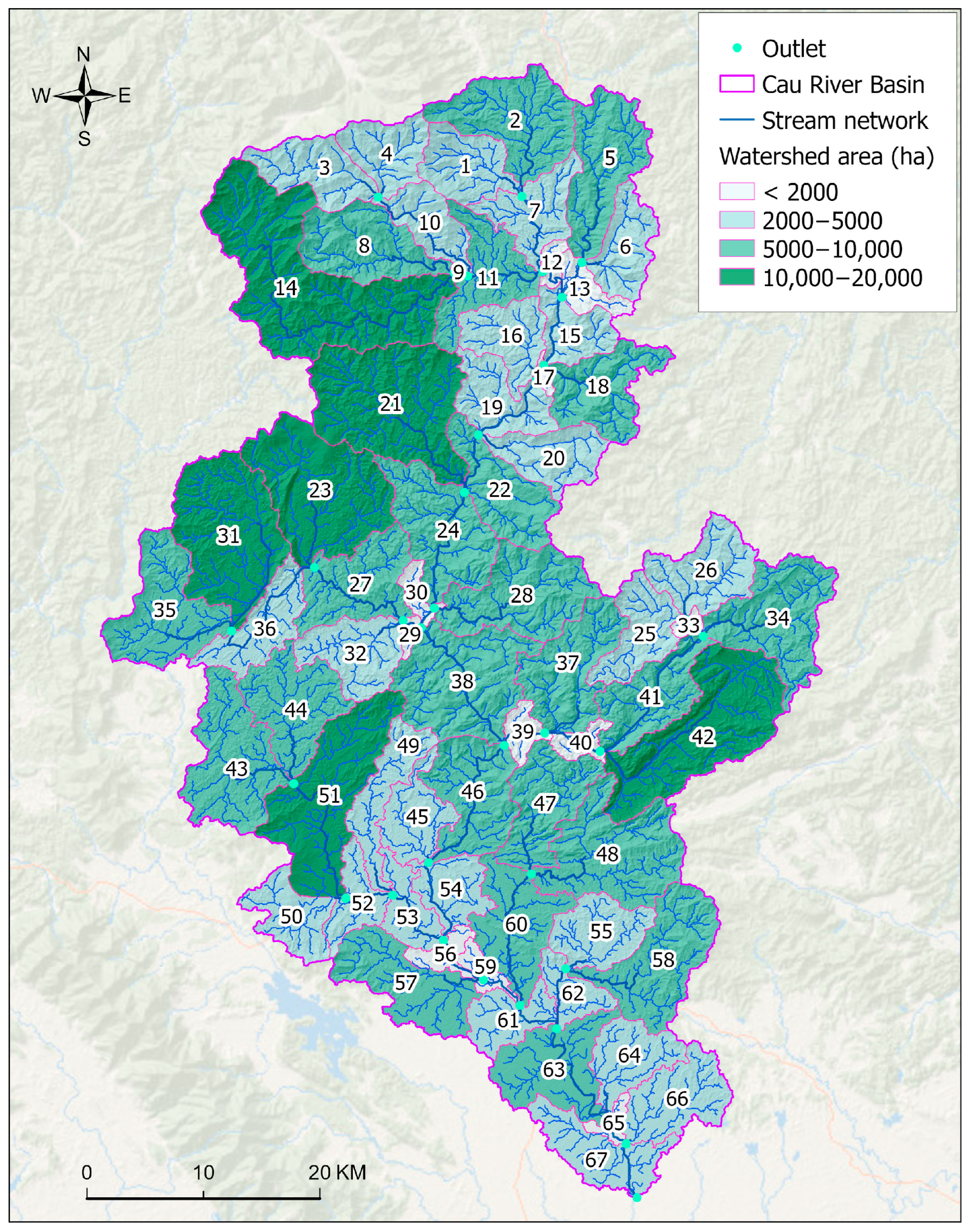
The 30-m resolution DEM was used to compute the stream network and delineate sub-watersheds using the Watershed Delineation tool in ArcSWAT. This procedure relies on flow direction and flow accumulation algorithms derived from the DEM, assuming that water flows from higher to lower elevation cells following the steepest descent [40,43]. As a result, the Cau River Basin was divided into 67 sub-watersheds, with sub-watershed 14 being the largest, covering an area of approximately 18,000 ha (Figure 4). Each sub-watershed was assigned a unique identifier and can be independently simulated within the model.
HRUs serve as the fundamental spatial units for simulating hydrological processes in SWAT. Each HRU represents a unique combination of LULC, soil type, and slope class within a sub-watershed (Figure 3). The HRU Definition module in ArcSWAT allows users to set threshold values to exclude spatial classes that occupy only a small proportion of the area and have limited hydrological impact. In this study, thresholds of 10% were applied for LULC, soil type, and slope to eliminate minor categories. This process resulted in the creation of 683 HRUs across the 67 sub-watersheds. Each HRU serves as the smallest spatial modelling unit in the SWAT framework, confirming its status as a semi-distributed hydrological model.
Following HRU analysis, meteorological data, including daily precipitation and temperature (maximum and minimum), were integrated into the model. After all required inputs were loaded, the model was executed to simulate streamflow at the sub-watershed outlets. The simulation period was set from 1990 to 2020, with the first three years (1990–1992) designated as the warm-up period to initialise model conditions. The warm-up period was included to initialise the model and allow it to reach stable, realistic starting conditions for key variables, as recommended in hydrological modelling practice [44]. This 31-year period was chosen based on the availability and continuity of reliable daily meteorological and hydrological data across the study area. It also provides a sufficiently long timeframe to capture interannual climatic variability and support robust model calibration, validation, and streamflow trend analysis.
Model calibration and validation are essential components of the hydrological modelling process, ensuring that simulated outputs reliably represent observed hydrological behaviour. SWAT model calibration involves adjusting key input parameters within defined ranges to minimise the discrepancy between simulated and observed streamflow, while validation tests the model’s performance against independent data to evaluate its predictive capability [35]. Based on our data availability, the model was calibrated for the period 1997–2008 and validated for the period 2009–2020 using observed streamflow at the Gia Bay hydrological station. Details of these processes are presented in the sections below.

2.4. Sensitivity Analysis, Calibration and Validation

Sensitivity analysis is conducted to identify and rank the most influential hydrological parameters that significantly affect the model output. Model calibration involves adjusting input parameters to ensure the simulation results align with observed data within acceptable ranges, thereby reducing predictive uncertainty. In contrast, validation tests the performance of the calibrated model using an independent dataset, without making further changes to the parameters [35]. The sensitivity analysis and calibration processes were automatically implemented using the SWAT-CUP (SWAT Calibration and Uncertainty Procedures) software (version 5.1.6.2), specifically employing the SUFI-2 (Sequential Uncertainty Fitting Version 2) algorithm [36]. SWAT-CUP facilitates automated calibration through iterative optimisation, offering a more efficient and statistically robust alternative to manual trial-and-error methods [45,46].
To guide calibration and reduce model uncertainty, a global sensitivity analysis was first conducted on ten key parameters that represent major hydrological processes in the Cau River basin (Table 1). These include parameters related to surface runoff, evaporation, infiltration and soil moisture capacity, groundwater dynamics, and surface flow routing. The selection of these parameters was based on three main criteria: (i) their direct influence on core hydrological processes such as runoff generation, baseflow, evapotranspiration, and water movement; (ii) recommendations from the SWAT-CUP documentation and prior calibration experience [36,47,48]; (iii) the need to adequately represent all components of the watershed’s water balance.
The sensitivity analysis was performed using 500 simulation runs, with t-stat and p-value statistics used to rank the parameters based on their influence. Parameters with high t-stat values and low p-values (<0.05) were identified as the most sensitive and were given priority during calibration. This approach ensures that calibration efforts focus on the most impactful variables, improving model accuracy while reducing computational time. Parameter value ranges were defined based on SWAT theoretical guidelines, physical characteristics of the Cau River Basin, and expert judgment to avoid unrealistic values and overfitting. Model calibration was performed for the period of 1997–2008 following the identification of the most sensitive parameters. Once calibrated, these optimised parameters were retained for all subsequent simulations, ensuring consistency and reliability in model outputs.
Following calibration, the SWAT model was validated using an independent time series (2009–2020) to assess its performance and generalisability under different climatic conditions. Comparing simulated and observed streamflow during this period helped evaluate the model’s stability, accuracy, and suitability for future hydrological analyses and water resource planning.

2.5. Model Performance Metrics

Model performance was quantitatively assessed using four statistical metrics widely used in previous studies [36,49,50]. These metrics included Nash–Sutcliffe Efficiency (NSE) [51], Percent Bias (PBIAS) [49], coefficient of determination (R2) [52], and Root Mean Square Error (RMSE) for observed Standard deviation Ratio (RSR) [49]. Each metric evaluates a specific aspect of model performance, from correlation strength and agreement with observations to systematic bias and model uncertainty. The use of multiple metrics allows for a comprehensive evaluation of model performance and supports robust conclusions on the reliability of the simulation results [15].
NSE is widely regarded as the principal metric for assessing the agreement between simulated and observed streamflow [35]. An NSE value approaching 1 indicates strong model performance, with NSE = 1 representing a perfect match. PBIAS measures the average deviation between simulated and observed values, with values close to 0 indicating high accuracy. A positive PBIAS suggests model overestimation, while a negative value indicates underestimation. This metric provides insight into the overall bias in model predictions. R2 quantifies the proportion of variance in the observed data explained by the model. Higher R2 values indicate stronger correlation and better reproduction of streamflow variability [15,24,31,49,51]. Finally, RSR (ratio of the Root Mean Square Error to the standard deviation of observed data) combines both error magnitude and variability. Lower RSR values reflect better model performance [49]. These metrics were computed using the equations below:
N S E = 1 i = 0 n ( Q o b s , i Q s i m ) 2 i = 0 n ( Q o b s , i Q o b s ¯ ) 2
P B I A S = 100 × i = 0 n ( Q o b s Q s i m ) i i = 0 n ( Q o b s , i )
R 2 = i = 0 n ( Q o b s , i Q o b s ¯ ) ( Q s i m , i Q s i m ¯ ) 2 i = 0 n ( Q o b s , i Q o b s ¯ ) 2 i = 1 n ( Q s i m , i Q s i m ¯ ) 2
R S R = i = 0 n ( Q o b s Q s i m ) i 2 i = 0 n ( Q o b s , i Q o b s ¯ ) 2
where Qobs and Qsim are observed and simulated values, respectively, of a hydrological variable. The model was considered to meet baseline performance criteria if the following thresholds were achieved: NSE > 0.50, R2 > 0.70, PBIAS within ±15%, and RSR < 0.5 [49].

3. Results

3.1. Parameter Sensitivity Analysis

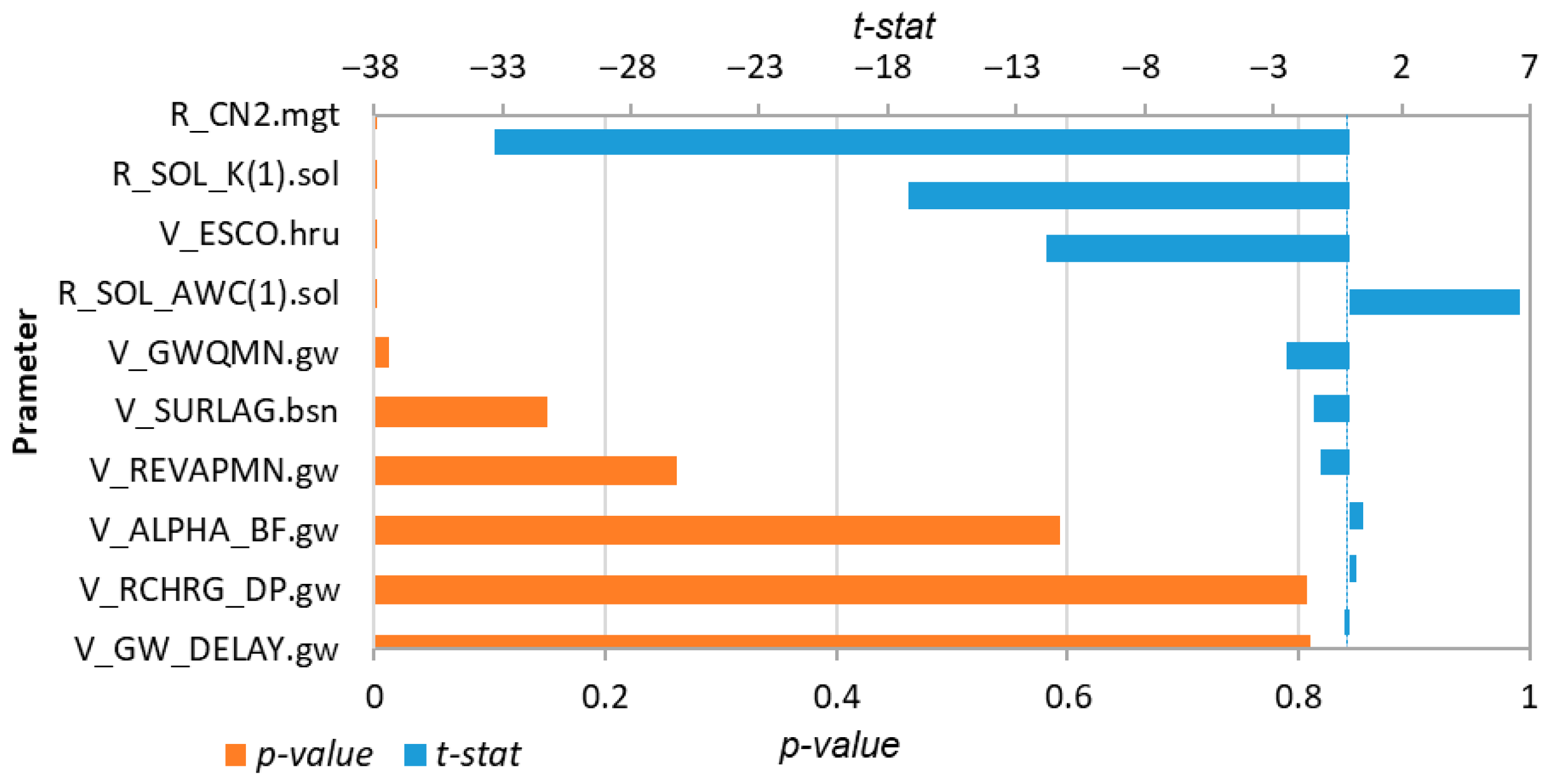
Results from the global sensitivity analysis indicate that four out of the ten analysed parameters were statistically significant (p < 0.05) and had the strongest influence on streamflow simulation (Figure 5). These included SOL_K.sol1 (t-stat = –17.2; p < 0.0001), CN2.mgt (t-stat = –33.3; p < 0.0001), ESCO.hru (t-stat = –11.8; p < 0.0001), and SOL_AWC.sol1 (t-stat = 6.6; p < 0.0001). These four parameters also showed a clear impact on model performance, as illustrated in Figure 6, confirming their high sensitivity and importance in the calibration process. The dot plots in Figure 6 represent the distribution of parameter values against corresponding NSE values. If the points are randomly scattered, the parameter is considered to have low sensitivity; in contrast, a clear trend in the data points indicates higher sensitivity, as changes in the parameter consistently influence NSE. The plots clearly show that CN2.mgt and SOL_K.sol exerted the greatest influence on NSE, followed by ESCO.hru and SOL_AWC.sol. Based on these results, the four most sensitive parameters were selected for model calibration. The final fitted parameters obtained from the SUFI-2 calibration of streamflow are presented in Table 2. Focusing on these key parameters improved calibration efficiency, reduced computational time, and enhanced model accuracy.

3.2. Model Performance

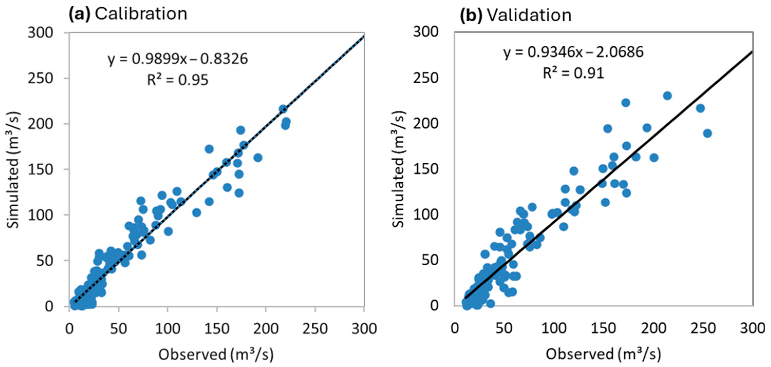
The accuracy of the SWAT model is summarised in Table 3 through key performance metrics. During the calibration period (1997–2008), the model achieved an NSE of 0.95, suggesting that 95% of the variance in observed streamflow was captured by the simulation. The R2 value was also 0.95, reflecting a strong linear relationship between simulated and observed data (Figure 7a). The PBIAS during calibration was 2.6%, and the RSR was 0.23. During the independent validation period (2009–2020), using the same calibrated parameter set, the model maintained a high level of performance. The NSE and R2 values remained high at 0.90 and 0.91, respectively (Table 3 and Figure 7b). However, both PBIAS and RSR during validation increased compared to the calibration phase, reaching 9.7% and 0.35, respectively.
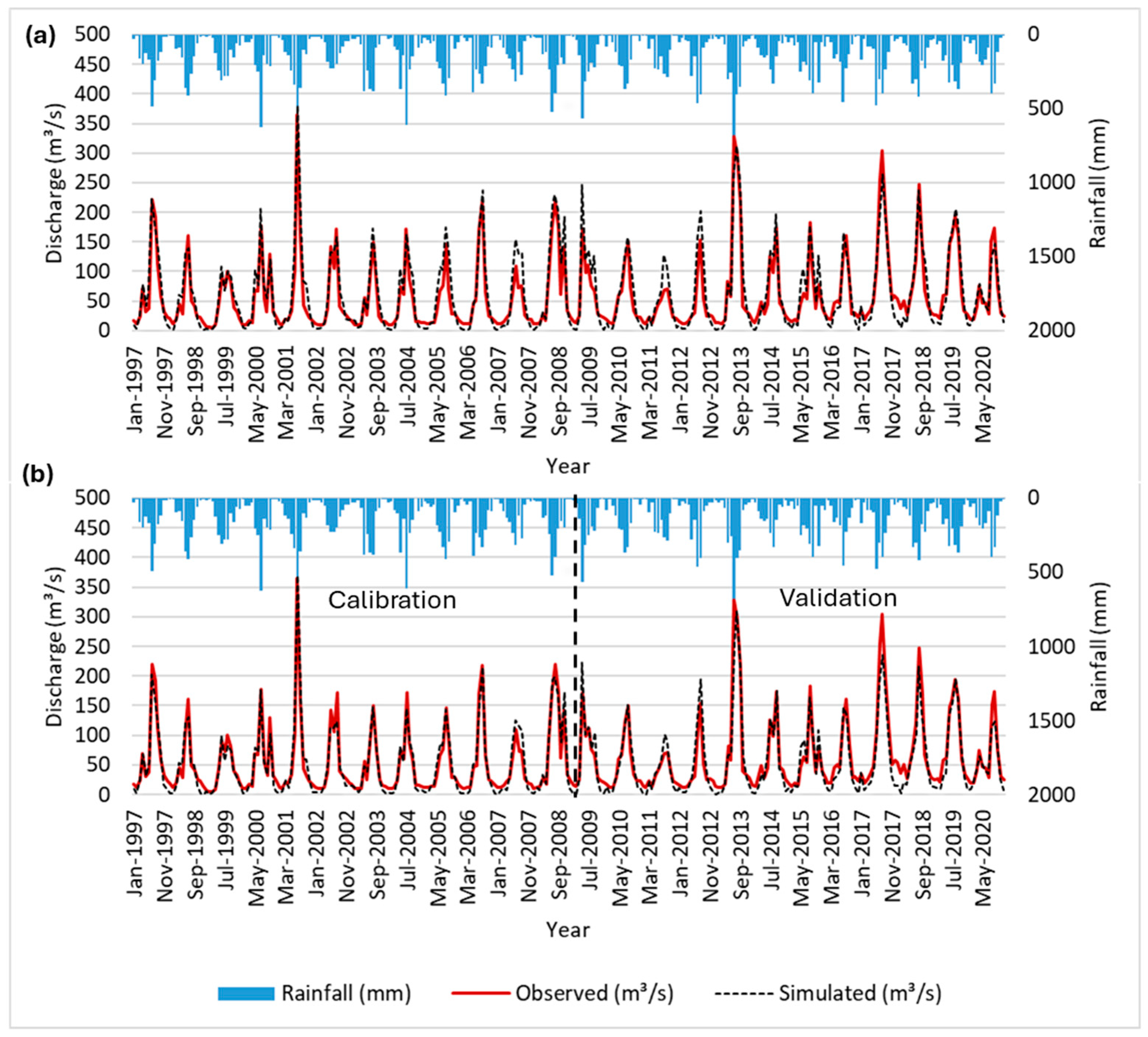
The temporal patterns of observed and simulated streamflow at Gia Bay station are shown in Figure 8. The initial (pre-calibrated) simulation results (Figure 8a) indicate that the pre-calibrated model reasonably reproduced the seasonal flow regime (R2 = 0.90, NSE = 0.87), capturing both the flood season (May–October) and the dry season (November–April). However, the model tended to underestimate peak flows in certain years (e.g., 2001, 2013, 2017) and slightly overestimate flows during low-flow periods. These discrepancies highlight the importance of calibrating sensitive parameters to improve the simulation of peak flow.
Following calibration, the simulation results were significantly improved (Figure 8b). Both flood and dry season flows were more consistently and accurately simulated across the calibration and validation periods. The calibrated model also captured seasonal variations more effectively, despite minor discrepancies in peak magnitudes during extreme years (e.g., 2001, 2013, 2017).

3.3. Spatio-Temporal Variation of Surface Runoff

3.3.1. Spatial Variation of Surface Runoff

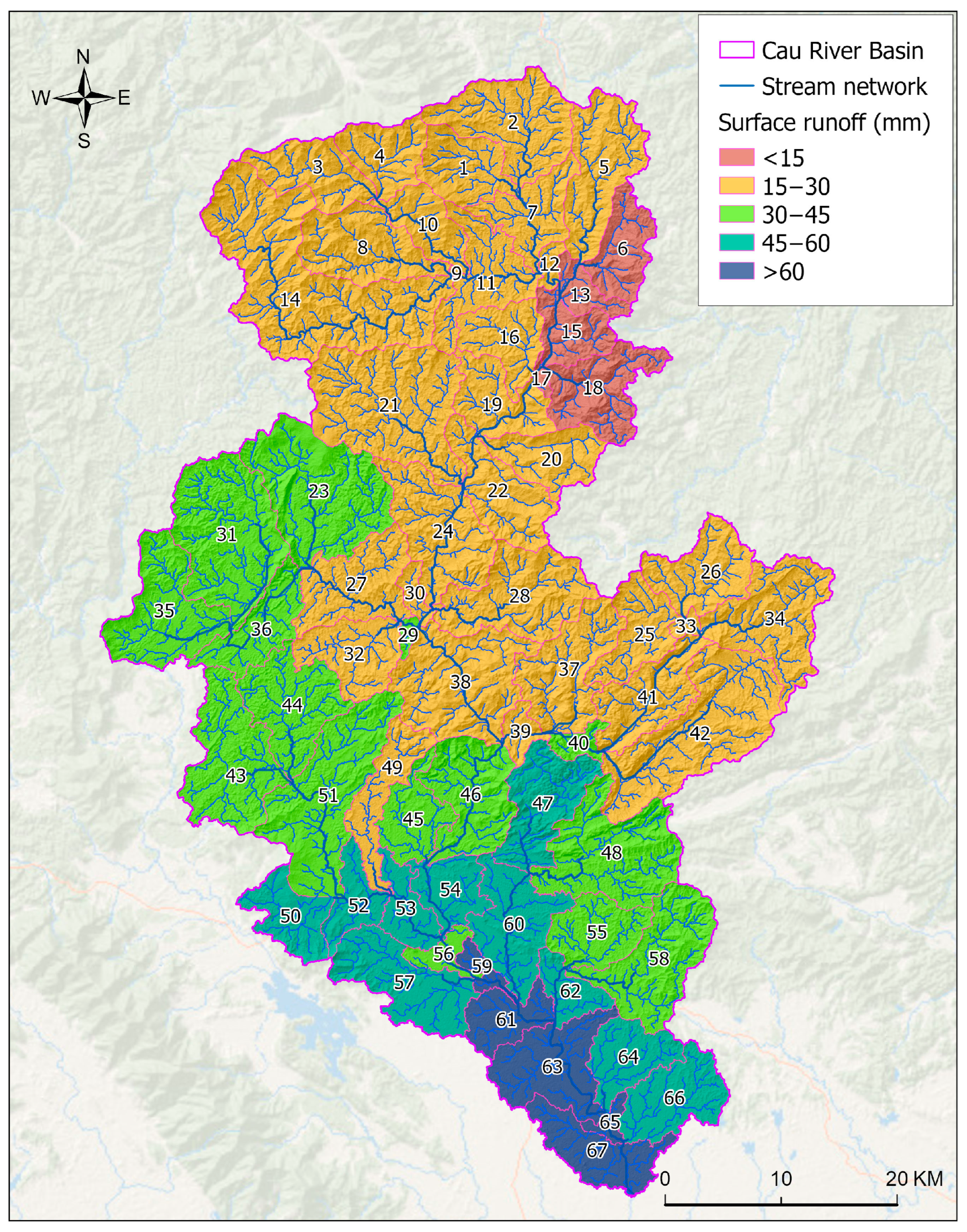
The spatial distribution of surface runoff across sub-watersheds in the Cau River Basin is presented in Figure 9. The simulation results showed significant spatial variability in surface runoff. Average annual surface runoff, computed across 67 sub-watersheds, ranged from 12.69 mm to 75.32 mm, with most sub-watersheds falling within the 20–40 mm range. Lower runoff values (<45 mm) were primarily recorded for upstream sub-watersheds, while higher runoff values (≥45 mm) were observed for downstream areas. Sub-watersheds 59, 61, 63, 65, and 67 were identified as runoff “hotspots,” with annual runoff exceeding 60 mm. Conversely, sub-watersheds 6, 13, 15, 17, and 18 recorded the lowest runoff values, all below 15 mm (Figure 9).

3.3.2. Temporal Variation of Surface Runoff

The average annual surface runoff in the Cau River Basin varied from 19.8 mm (2011) to 56.4 mm (2013), with a long-term average of approximately 32.4 mm (Figure 10a). Years such as 2001, 2008, 2013, and 2019 recorded unusually high surface runoff, while the period from 2011 to 2016 featured below-average runoff and the lowest year in the series. The analysis also revealed strong seasonality in surface runoff patterns, typical of a humid tropical monsoon climate (Figure 10b). During the dry season (November to April), surface runoff is minimal, with some months approaching near-zero values, indicating severe surface water depletion due to lack of rainfall. In contrast, runoff increases sharply during the wet season (May to October), especially during June to September, which coincides with peak rainfall months. Some months experienced extreme surface runoff, including July 2001 (282.15 mm), July 2013 (279.23 mm), May 2009 (209.46 mm), and August 2018 (171.06 mm). Furthermore, several years such as 1995 and 1998 exhibited low runoff across most months (Figure 10b).

4. Discussions

This study successfully developed and calibrated a SWAT model for the Cau River Basin by integrating geospatial datasets, including DEM, soil, and LULC, with historical climate records. The model produced strong calibration and validation results, effectively capturing both spatial and temporal variations in streamflow across the basin.
The SWAT model demonstrated consistent performance in simulating streamflow dynamics during both the calibration (1997–2008) and validation (2009–2020) periods. The model achieved NSE and R2 values exceeding 0.9 in both phases (Table 3), indicating strong agreement between simulated and observed streamflow. Although PBIAS and RSR increased during validation (from 2.6% to 9.7% for PBIAS, and from 0.23 to 0.35 for RSR) both remained well within the acceptable thresholds recommended by previous studies (PBIAS within ±15%, RSR < 0.5) [49,53]. These results suggest that the model reliably simulates streamflow with low systematic error and maintains stable performance across different hydrological periods.
Our model results are comparable to those reported by previous SWAT modelling studies of the Cau River Basin [e.g., 15,16,17]. For example, Dao, Lu, Chen, Kantoush, Binh, Phan and Tung [16] developed SWAT models for the basin using modelled meteorological products (spatial resolution from 0.25 to 0.31 degree) and obtained slightly lower performance, with NSE values of 0.78–0.81 and R2 values of 0.78–0.85. This highlights the advantage of using observed weather data in the present study. In another study, Thai, Thao and Dieu [17] NSE values were 0.85 and 0.81 for the calibration (1991–1999) and validation (1980–1990) periods, respectively. Although they also used station-based meteorological data, their model inputs included a coarser 90 m DEM (compared to 30 m in our study) and a Landsat-derived LULC map (30 m), which may have limited their model’s performance [17]. The slightly improved results in our study can therefore be attributed to the integration of higher-resolution DEM and more accurate LULC data (created from cadastral maps and field surveys). Our findings are also consistent with SWAT applications in other humid tropical and monsoon-dominated catchments (e.g., [3,13,54]). For instance, Chakraborty, Saha and Mandal [13] reported R2 values ranging from 0.82 to 0.93 for eight stations across the Ganga basin, India. Similarly, Singh, Kanga, Gulati, Raič, Sajan, Đurin and Singh [54] yielded NSE values of 0.88 and 0.82 for calibration and validation in the Beas River Basin, which are comparable to those achieved in this study. These results confirm the robustness of the SWAT model when supported by high-quality input data and rigorous calibration procedures.
The sensitivity analysis identified CN2.mgt, SOL_K.sol1, ESCO.hru, and SOL_AWC.sol1 as the most influential parameters governing streamflow simulation. The calibrated values reflect realistic watershed characteristics, with moderate adjustments to curve number and soil hydraulic properties (Figure 5, Table 2). Calibrated values were optimised within physically reasonable ranges, consistent with guidelines for SWAT calibration [35,36]. These results were expected, as these parameters are particularly sensitive to LULC and soil properties, making them crucial for hydrological modelling in transitional or rapidly urbanising basins such as the Cau River Basin. Specifically, the saturated hydraulic conductivity of the topsoil layer (SOL_K.sol1) directly influences the balance between surface runoff and infiltration. The curve number (CN2.mgt), determined by factors such as soil type, texture, permeability, and land use characteristics, controls the amount of surface runoff generated from precipitation events [48,55]. The soil evaporation compensation factor (ESCO.hru) regulates evapotranspiration from the upper soil layer and influences soil moisture retention, while the available water capacity of the topsoil (SOL_AWC.sol1) determines the soil’s capacity to store water between rainfall events [55,56]. These findings are consistently supported by previous studies [10,22,24,46,55,56,57], which have also identified CN2 and SOL_K as dominant factors influencing runoff partitioning and infiltration dynamics, alongside SOL_AWC and ESCO. It is also important to note that previous studies in the Cau River Basin did not explicitly identify the dominant parameters that substantially influence streamflow simulation [16,17]. These findings highlight that soil hydraulic properties and LULC-driven runoff potential are the key factors influencing flow generation. This underscores the critical role of incorporating detailed soil and LULC datasets in modelling efforts for hydrologically complex and rapidly changing basins.
The spatial variability of surface runoff across the Cau River Basin reflects the combined influences of topography, vegetation cover, and land use practices (Figure 9). Sub-watersheds with low runoff values (<45 mm) are typically located in areas with high infiltration capacity, denser vegetation, and more sustainable agricultural management, which reduce surface runoff. In contrast, higher runoff levels (≥45 mm) are often associated with steep slopes, degraded vegetation, or urbanisation, where increased impervious surfaces limit infiltration. These findings provide a basis for prioritising soil conservation efforts, improving land use planning, and developing targeted management strategies to enhance watershed resilience.
The variability in annual runoff (Figure 10a) reflects the instability of the basin’s hydrological regime, driven by both climatic and land use changes. Years with unusually high runoff, such as 2001, 2008, 2013, and 2019, likely correspond to extreme weather events like prolonged heavy rainfall or major shifts in land use. In contrast, the below-average runoff observed between 2011 and 2016 may be attributed to reduced rainfall combined with improved infiltration capacity due to more permeable land cover during that period [58,59]. These findings align with Thai, Thao and Dieu [17], who reported increased erosion and runoff in the upper Cau Basin under climate change and land use change scenarios. The pronounced seasonality of surface runoff (Figure 10b) highlights the basin’s sensitivity to monsoon rainfall patterns. The occurrence of extreme runoff months, such as in July 2001 and July 2013, reflects the basin’s rapid hydrological response to intense rainfall events. We also observed a noticeable increase in wet-season runoff (since 2001), which could be linked to land use changes (e.g., urbanisation or increased impervious surfaces) and alterations in rainfall distribution patterns potentially associated with climate change [7,18,60,61]. These findings provide important insights for water resource planning, flood risk management, and climate adaptation strategies in the Cau River Basin.
While the SWAT model performed well in simulating streamflow in the Cau River Basin, several limitations should be acknowledged. First, the model calibration and validation relied solely on streamflow data from a single hydrological station (Gia Bay), as no additional discharge measurements were available within the study area. This limits the ability to assess flow variability across the basin and constrains spatial representativeness. Future studies in data-scarce regions should consider integrating remote sensing products or hydrological proxies to improve spatial calibration. Second, the model underestimated peak flows during major flood events (e.g., 2001, 2013, 2017), likely due to limited spatial coverage of rainfall data. This is a well-documented challenge in SWAT applications, particularly in mountainous or convective-storm-dominated regions [10,20]. In the Cau River Basin, the highly dissected terrain leads to the formation of multiple microclimates, resulting in significant spatial variability in rainfall. Incorporating high-resolution gridded rainfall datasets or satellite-based precipitation products would improve the model’s capacity to capture hydrological extremes. Third, the use of a static LULC map from 2020 for the entire simulation period (1990–2020) ignores historical land use changes such as urbanisation, agricultural expansion, and reforestation. This may have introduced errors in surface runoff simulation, particularly in rapidly changing areas. Updating the model with time-series LULC data from remote sensing products would allow for a more accurate representation of land use impacts on hydrological processes. Finally, human interventions, including irrigation systems, groundwater extraction, and flow diversions, were not accounted for in the model. Although no large reservoirs had been constructed in the study area by 2021, many small-scale farm ponds have been developed locally for domestic water use and irrigation. Unfortunately, data on their number, capacity, and spatial distribution are currently unavailable due to the lack of official records. Collecting such data and incorporating ponds and reservoir operations into future simulations would further improve model accuracy and reliability for water resource management.

5. Conclusions

This study successfully developed and calibrated a SWAT model for the Cau River Basin, in northeast Vietnam, by integrating spatial data (DEM, soil, and LULC) with historical climate records. The model achieved high calibration and validation performance, with NSE > 0.90 and R2 > 0.91, confirming its capacity to simulate both the magnitude and seasonal dynamics of streamflow with minimal bias. The analysis revealed substantial spatio-temporal variability in surface runoff, with annual runoff ranging from 19.8 mm in 2011 to 56.4 mm in 2013. Runoff was generally higher in downstream sub-watersheds (>60 mm) and lower in upstream areas (<30 mm), while seasonal contrasts between wet and dry periods were clearly reproduced. These results provide crucial insights for flood and drought risk assessment, especially in the context of changing rainfall patterns and land use pressures. The sensitivity analysis identified four key hydrological parameters (curve number, saturated hydraulic conductivity, soil evaporation compensation factor, and available water capacity) as primary drivers of streamflow dynamics. This finding underscores the need for detailed soil and land cover data in hydrological modelling, particularly for basins experiencing rapid urbanisation or land cover change.
The calibrated SWAT model offers a practical decision-support tool for regional water resource management. It can be applied to simulate future land use and climate change scenarios, providing critical information to guide sustainable land management and urban planning policies. Additionally, the model supports evidence-based flood mitigation strategies by identifying runoff hotspots and prioritising areas for soil conservation or reforestation. It also aids drought management and water allocation planning by quantifying water availability under varying climatic conditions, ensuring more resilient and adaptive resource management practices.
For future research, the model should be expanded to include sediment yield and water quality components, enabling more comprehensive assessments of erosion risks and pollution transport. Incorporating time-series LULC data and high-resolution rainfall inputs will further improve model accuracy. Additionally, integrating human interventions, such as reservoir operations and groundwater abstraction, will enhance the model’s applicability for adaptive and integrated watershed management in the Cau River Basin.

Author Contributions

Conceptualization, N.A.N., V.T.C. and T.H.N.; methodology, N.A.N., V.T.C. and T.H.N.; software, N.A.N. and V.T.C.; validation, N.A.N. and V.T.C.; formal analysis, N.A.N. and V.T.C.; investigation, N.A.N.; resources, N.A.N., V.T.C. and T.H.N.; data curation, N.A.N. and V.T.C.; writing—original draft preparation, N.A.N., V.T.C. and T.H.N.; writing—review and editing, L.H.N., A.T.H.; visualization, N.A.N. and T.H.N.; supervision, T.H.N.; project administration, N.A.N.; funding acquisition, N.A.N. All authors have read and agreed to the published version of the manuscript.

Funding

This work was financially supported by Vietnam Ministry of Education and Training under project number: B2024-TNA-15.

Data Availability Statement

The original contributions presented in the study are included in the article, further inquiries can be directed to the corresponding author.

Acknowledgments

We would like to express our deepest gratitude and remembrance for Phan Dinh Binh (Faculty of Resource Management, University of Agriculture and Forestry—Thai Nguyen University), who initiated the research idea and was the original principal investigator of this project. Although he sadly passed away, his invaluable contributions and unwavering dedication remain a foundational part of this study and continue to inspire its completion.

Conflicts of Interest

The authors declare no conflicts of interest.

Abbreviations

The following abbreviations are used in this manuscript:
GISGeographic Information System
ArcSwatArcGIS interface for the Soil and Water Assessment Tool
DEMDigital Elevation Model
FAOFood and Agriculture Organisation
HWSDHarmonised World Soil Database
HRUHydrologic Response Unit
LULCLand Use and Land Cover
NSENash–Sutcliffe Efficiency
PBIASPercent Bias
R2Coefficient of determination
RMSERoot Mean Square Error
RSRRoot Mean Square Error to observations Standard deviation Ratio
SWATSoil and Water Assessment Tool
SWAT-CUPSWAT–Calibration and Uncertainty Procedures
SUFI-2Sequential Uncertainty Fitting ver. 2
SRTMShuttle Radar Topography Mission
USGSUnited States Geological Survey

References

  1. Davie, T. Fundamentals of Hydrology; Routledge: London, UK, 2019. [Google Scholar]
  2. Wang, Y.; Jiang, R.; Xie, J.; Zhao, Y.; Yan, D.; Yang, S. Soil and water assessment tool (SWAT) model: A systemic review. J. Coast. Res. 2019, 93, 22–30. [Google Scholar] [CrossRef]
  3. Janjić, J.; Tadić, L. Fields of application of SWAT hydrological model—A review. Earth 2023, 4, 331–344. [Google Scholar] [CrossRef]
  4. Yang, D.; Yang, Y.; Xia, J. Hydrological cycle and water resources in a changing world: A review. Geogr. Sustain. 2021, 2, 115–122. [Google Scholar] [CrossRef]
  5. Biggs, D.; Miller, F.; Hoanh, C.T.; Molle, F. The delta machine: Water management in the Vietnamese Mekong Delta in historical and contemporary perspectives. In Contested Waterscapes in the Mekong Region; Routledge: London, UK, 2012; pp. 203–225. [Google Scholar]
  6. Pham, Q.-N.; Nguyen, N.-H.; Ta, T.-T.; Tran, T.-L. Vietnam’s water resources: Current status, challenges, and security perspective. Sustainability 2023, 15, 6441. [Google Scholar] [CrossRef]
  7. Wada, Y.; Bierkens, M.F.; De Roo, A.; Dirmeyer, P.A.; Famiglietti, J.S.; Hanasaki, N.; Konar, M.; Liu, J.; Müller Schmied, H.; Oki, T. Human–water interface in hydrological modelling: Current status and future directions. Hydrol. Earth Syst. Sci. 2017, 21, 4169–4193. [Google Scholar] [CrossRef]
  8. Fiener, P.; Auerswald, K.; Van Oost, K. Spatio-temporal patterns in land use and management affecting surface runoff response of agricultural catchments—A review. Earth-Sci. Rev. 2011, 106, 92–104. [Google Scholar] [CrossRef]
  9. Singh, V. Effect of spatial and temporal variability in rainfall and watershed characteristics on stream flow hydrograph. Hydrol. Process. 1997, 11, 1649–1669. [Google Scholar] [CrossRef]
  10. Swain, S.; Mishra, S.; Pandey, A.; Pandey, A.; Jain, A.; Chauhan, S.; Badoni, A.K. Hydrological modelling through SWAT over a Himalayan catchment using high-resolution geospatial inputs. Environ. Chall. 2022, 8, 100579. [Google Scholar] [CrossRef]
  11. Iqbal, S.; Haider, R.; Pasha, G.A.; Zhao, L.; Abbas, F.M.; Anjum, N.; Murtaza, N.; Abbas, Z. Numerical Investigation of Flow Around Partially and Fully Vegetated Submerged Spur Dike. Water 2025, 17, 435. [Google Scholar] [CrossRef]
  12. Himanshu, S.K.; Pandey, A.; Yadav, B.; Gupta, A. Evaluation of best management practices for sediment and nutrient loss control using SWAT model. Soil Tillage Res. 2019, 192, 42–58. [Google Scholar] [CrossRef]
  13. Chakraborty, K.; Saha, S.; Mandal, D. Hydrological modelling using SWAT for the assessment of streamflow dynamics in the Ganga River basin. Environ. Sci. Pollut. Res. 2024, 32, 10258–10278. [Google Scholar] [CrossRef]
  14. Sharma, U.; Sharma, V.; Eslamian, S. Flood Management; Larsen and Keller Education: New York, NY, USA, 2022; p. 79. [Google Scholar]
  15. Bui, H.H.; Ha, N.H.; Nguyen, T.N.D.; Nguyen, A.T.; Pham, T.T.H.; Kandasamy, J.; Nguyen, T.V. Integration of SWAT and QUAL2K for water quality modeling in a data scarce basin of Cau River basin in Vietnam. Ecohydrol. Hydrobiol. 2019, 19, 210–223. [Google Scholar] [CrossRef]
  16. Dao, D.M.; Lu, J.; Chen, X.; Kantoush, S.A.; Binh, D.V.; Phan, P.; Tung, N.X. Predicting tropical monsoon hydrology using CFSR and CMADS data over the Cau River Basin in Vietnam. Water 2021, 13, 1314. [Google Scholar] [CrossRef]
  17. Thai, T.H.; Thao, N.P.; Dieu, B.T. Assessment and simulation of impacts of climate change on erosion and water flow by using the soil and water assessment tool and GIS: Case Study in Upper Cau River basin in Vietnam. Earth Sci. 2017, 39, 376–392. [Google Scholar] [CrossRef]
  18. Tran, V.-B.; Ishidaira, H.; Nakamura, T.; Do, T.-N.; Nishida, K. Estimation of nitrogen load with multi-pollution sources using the SWAT model: A case study in the Cau River Basin in Northern Vietnam. J. Water Environ. Technol. 2017, 15, 106–119. [Google Scholar] [CrossRef]
  19. Son, C.T.; Giang, N.T.H.; Thao, T.P.; Nui, N.H.; Lam, N.T.; Cong, V.H. Assessment of Cau River water quality assessment using a combination of water quality and pollution indices. J. Water Supply Res. Technol.—AQUA 2020, 69, 160–172. [Google Scholar] [CrossRef]
  20. Hien, H.N.; Hoang, B.H.; Huong, T.T.; Than, T.T.; Ha, P.T.T.; Toan, T.D.; Son, N.M. Study of the climate change impacts on water quality in the upstream portion of the cau river basin, vietnam. Environ. Model. Assess. 2016, 21, 261–277. [Google Scholar] [CrossRef]
  21. Le, T.T.T.; Kawagoe, S. Evaluation of landslide susceptibility in Cau River Basin using a physical-based model under impact of climate change. Open J. Mod. Hydrol. 2018, 9, 1. [Google Scholar]
  22. Mohseni, U.; Agnihotri, P.G.; Pande, C.B.; Durin, B. Understanding the climate change and land use impact on streamflow in the present and future under CMIP6 climate scenarios for the Parvara Mula Basin, India. Water 2023, 15, 1753. [Google Scholar] [CrossRef]
  23. Devia, G.K.; Ganasri, B.P.; Dwarakish, G.S. A review on hydrological models. Aquat. Procedia 2015, 4, 1001–1007. [Google Scholar] [CrossRef]
  24. Bo, H.; Dong, X.; Li, Z.; Reta, G.; Li, L.; Wei, C. Comparison of Two Versions of SWAT Models in Predicting the Streamflow in the Xuanmiaoguan Reservoir Catchment. Nat. Environ. Pollut. Technol. 2022, 21, 529–541. [Google Scholar] [CrossRef]
  25. Arnold, J.G.; Srinivasan, R.; Muttiah, R.S.; Williams, J.R. Large area hydrologic modeling and assessment part I: Model development 1. JAWRA J. Am. Water Resour. Assoc. 1998, 34, 73–89. [Google Scholar] [CrossRef]
  26. Liu, H.; Wang, T.; Feng, Y.; Liu, F.; Wang, N.; Wang, H.; Liu, W.; Sun, F. Identifying Reservoir-Induced Hydrological Alterations in the Upper Yangtze River Basin through Statistical and Modeling Approaches. Water 2023, 15, 2914. [Google Scholar] [CrossRef]
  27. Mwitalemi, S.S.; Kantoush, S.A.; Nguyen, B.Q. Effects of Cascading Dams on Streamflow within the Downstream Areas of the Rufiji River Basin in Tanzania. Hydrology 2024, 11, 69. [Google Scholar] [CrossRef]
  28. Wang, G.; Mang, S.; Cai, H.; Liu, S.; Zhang, Z.; Wang, L.; Innes, J.L. Integrated watershed management: Evolution, development and emerging trends. J. For. Res. 2016, 27, 967–994. [Google Scholar] [CrossRef]
  29. Doost, Z.H.; Alsuwaiyan, M.; Yaseen, Z.M. Runoff management based water harvesting for better water resources sustainability: A comprehensive review. Knowl.-Based Eng. Sci. 2024, 5, 1–45. [Google Scholar] [CrossRef]
  30. Jiang, D.; Wang, K. The role of satellite-based remote sensing in improving simulated streamflow: A review. Water 2019, 11, 1615. [Google Scholar] [CrossRef]
  31. Bach, T.V. Application of the SWAT Model for Simulating Streamflow and Sediment Yield. J. Water Resour. Environ. Eng. 2017, 57, 136–142. [Google Scholar]
  32. MONRE. Vietnam National Environmental Report 2006: Status of Three Water Basin: Cau River, Nhue–Day River and Dong Nai River; Ministry of Natural Resources and Environment: Hanoi, Vietnam, 2006. [Google Scholar]
  33. Quy, L.D. Developing flood inundation maps of Bac Thai caused by flooding from the Cau River and Cong River. J. Meteorol. Hydrol. 1990, 353, 15–23. [Google Scholar]
  34. Duong Thi, L.; Do Van, T.; Le Van, H. Detection of flash-flood potential areas using watershed characteristics: Application to Cau River watershed in Vietnam. J. Earth Syst. Sci. 2020, 129, 120. [Google Scholar] [CrossRef]
  35. Arnold, J.G.; Moriasi, D.N.; Gassman, P.W.; Abbaspour, K.C.; White, M.J.; Srinivasan, R.; Santhi, C.; Harmel, R.; Van Griensven, A.; Van Liew, M.W. SWAT: Model use, calibration, and validation. Trans. ASABE 2012, 55, 1491–1508. [Google Scholar] [CrossRef]
  36. Abbaspour, K.C. SWAT-CUP: SWAT calibration and uncertainty programs—A user manual. Eawag 2015, 100, 16–70. [Google Scholar]
  37. Zandbergen, P. Applications of shuttle radar topography mission elevation data. Geogr. Compass 2008, 2, 1404–1431. [Google Scholar] [CrossRef]
  38. Rabus, B.; Eineder, M.; Roth, A.; Bamler, R. The shuttle radar topography mission—A new class of digital elevation models acquired by spaceborne radar. ISPRS J. Photogramm. Remote Sens. 2003, 57, 241–262. [Google Scholar] [CrossRef]
  39. Moradkhani, H.; Sorooshian, S. General review of rainfall-runoff modeling: Model calibration, data assimilation, and uncertainty analysis. In Hydrological Modelling the Water Cycle: Coupling the Atmospheric Hydrological Models; Springer: Berlin/Heidelberg, Germany, 2009; pp. 1–24. [Google Scholar]
  40. Neitsch, S.L.; Arnold, J.G.; Kiniry, J.R.; Williams, J.R.; King, K. Soil and Water Assessment Tool: Theoretical Documentation: Version 2005; Grassland Soil and Water Research Laboratory: Temple, TX, USA, 2005. [Google Scholar]
  41. FAO; IIASA. Harmonized World Soil Database Version 2.0; FAO: Rome, Italy; IIASA: Laxenburg, Austria, 2023. [Google Scholar] [CrossRef]
  42. Poggio, L.; De Sousa, L.M.; Batjes, N.H.; Heuvelink, G.B.; Kempen, B.; Ribeiro, E.; Rossiter, D. SoilGrids 2.0: Producing soil information for the globe with quantified spatial uncertainty. Soil 2021, 7, 217–240. [Google Scholar] [CrossRef]
  43. Kaliappan, S.; Venkatraman, V. Determination of parameters for watershed delineation using various satellite derived digital elevation models and its accuracy. Glob. Nest J. 2023, 25, 124–137. [Google Scholar]
  44. Kim, K.B.; Kwon, H.-H.; Han, D. Exploration of warm-up period in conceptual hydrological modelling. J. Hydrol. 2018, 556, 194–210. [Google Scholar] [CrossRef]
  45. Wu, H.; Chen, B. Evaluating uncertainty estimates in distributed hydrological modeling for the Wenjing River watershed in China by GLUE, SUFI-2, and ParaSol methods. Ecol. Eng. 2015, 76, 110–121. [Google Scholar] [CrossRef]
  46. Zhao, F.; Wu, Y.; Qiu, L.; Sun, Y.; Sun, L.; Li, Q.; Niu, J.; Wang, G. Parameter uncertainty analysis of the SWAT model in a mountain-loess transitional watershed on the Chinese Loess Plateau. Water 2018, 10, 690. [Google Scholar] [CrossRef]
  47. Nossent, J. Sensitivity and Uncertainty Analysis in View of the Parameter Estimation of a SWAT Model of the River Kleine Nete, Belgium. Ph.D. Thesis, Vrije Universiteit Brussel, Brussels, Belgium, 2012. [Google Scholar]
  48. Arnold, J.; Kiniry, J.; Srinivasan, R.; Williams, J.; Haney, E.; Neitsch, S. Soil and Water Assessment Tool Input/Output File Documentation Version 2009; Texas Water Resources Institute: College Station, TX, USA, 2011. [Google Scholar]
  49. Moriasi, D.N.; Arnold, J.G.; Van Liew, M.W.; Bingner, R.L.; Harmel, R.D.; Veith, T.L. Model evaluation guidelines for systematic quantification of accuracy in watershed simulations. Trans. ASABE 2007, 50, 885–900. [Google Scholar] [CrossRef]
  50. Gupta, H.V.; Kling, H.; Yilmaz, K.K.; Martinez, G.F. Decomposition of the mean squared error and NSE performance criteria: Implications for improving hydrological modelling. J. Hydrol. 2009, 377, 80–91. [Google Scholar] [CrossRef]
  51. Nash, J.E.; Sutcliffe, J.V. River flow forecasting through conceptual models part I—A discussion of principles. J. Hydrol. 1970, 10, 282–290. [Google Scholar] [CrossRef]
  52. Yates, F. The analysis of multiple classifications with unequal numbers in the different classes. J. Am. Stat. Assoc. 1934, 29, 51–66. [Google Scholar] [CrossRef]
  53. Moriasi, D.N.; Gitau, M.W.; Pai, N.; Daggupati, P. Hydrologic and Water Quality Models: Performance Measures and Evaluation Criteria. Trans. ASABE 2015, 58, 1763–1785. [Google Scholar] [CrossRef]
  54. Singh, S.K.; Kanga, S.; Gulati, B.; Raič, M.; Sajan, B.; Đurin, B.; Singh, S. Spatial and temporal analysis of hydrological modelling in the Beas basin using SWAT+ model. Water 2023, 15, 3338. [Google Scholar] [CrossRef]
  55. Mengistu, D.; Sorteberg, A. Sensitivity of SWAT simulated streamflow to climatic changes within the Eastern Nile River basin. Hydrol. Earth Syst. Sci. 2012, 16, 391–407. [Google Scholar] [CrossRef]
  56. Leta, M.K.; Ebsa, D.G.; Regasa, M.S.; Shokrollahi, A. Parameter Uncertainty Analysis for Streamflow Simulation Using SWAT Model in Nashe Watershed, Blue Nile River Basin, Ethiopia. Appl. Environ. Soil Sci. 2022, 2022, 1826942. [Google Scholar] [CrossRef]
  57. Ashu, A.B.; Lee, S.-I. Multi-site calibration of hydrological model and spatio-temporal assessment of water balance in a monsoon watershed. Water 2023, 15, 360. [Google Scholar] [CrossRef]
  58. Department of Natural Resources and Environment of Thai Nguyen. Assessment of Land Use Change in Thai Nguyen During 2011–2020; Department of Natural Resources and Environment of Thai Nguyen: Thai Nguyen, Vietnam, 2021. [Google Scholar]
  59. Department of Natural Resources and Environment of Bac Kan. Assessment of Land Use Change in Bac Kan During 2011–2020; Department of Natural Resources and Environment of Bac Kan: Bac Kan, Vietnam, 2021. [Google Scholar]
  60. Blanco-Gómez, P.; Jimeno-Sáez, P.; Senent-Aparicio, J.; Pérez-Sánchez, J. Impact of climate change on water balance components and droughts in the Guajoyo River Basin (El Salvador). Water 2019, 11, 2360. [Google Scholar] [CrossRef]
  61. Kumar, A.; Singh, R.P.; Dubey, S.K.; Gaurav, K. Streamflow of the Betwa river under the combined effect of LU-LC and climate change. Agriculture 2022, 12, 2005. [Google Scholar] [CrossRef]
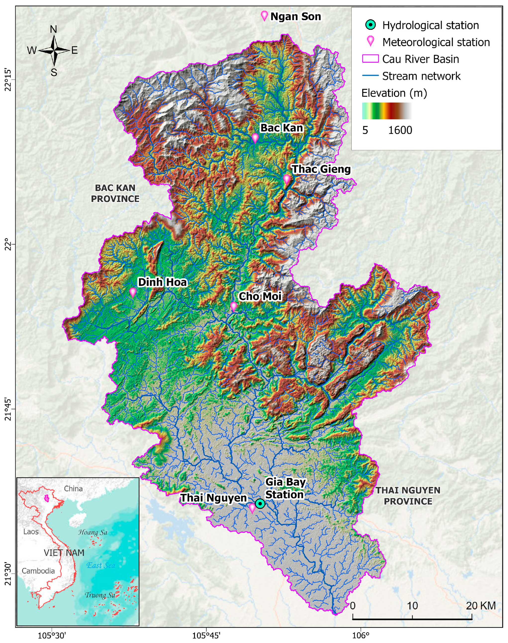
Figure 1. Study area within the Cau River Basin, northeastern Vietnam. The Cau River is highlighted as the thick blue line. Locations of meteorological and hydrological stations are also overlaid.
Geographies 05 00041 g001
Figure 2. Spatial data used in SWAT model. (a) Elevation, (b) Slope, (c) Soil type and (d) LULC map.
Geographies 05 00041 g002
Figure 3. Overall SWAT modelling framework.
Geographies 05 00041 g003
Figure 4. Sub-watersheds defined in Cau River Basin, categorised by their area.
Geographies 05 00041 g004
Figure 5. Sensitivity chart showing t-stat and p-value for each parameter considered in the SWAT calibration process. The prefixes R_ and V_ represents “relative” and “replace”, respectively, in SWAT-CUP.
Geographies 05 00041 g005
Figure 6. Dot plots showing distribution of selected parameter values (X-axis) against corresponding NSE values (Y-axis) during the SWAT calibration phase. Each green dot represents an individual simulation result, based on 500 simulations.
Geographies 05 00041 g006
Figure 7. Scatter plots showing linear relationships between simulated and observed streamflow at Gia Bay station for (a) calibration and (b) validation phases.
Geographies 05 00041 g007
Figure 8. Comparison of observed and simulated streamflow at monthly scale at Gia Bay station: (a) initial simulation before calibration, and (b) simulation after calibration.
Geographies 05 00041 g008
Figure 9. Spatial distribution of surface runoff across sub-watersheds in the Cau River Basin.
Geographies 05 00041 g009
Figure 10. (a) annual and (b) monthly variation of average surface runoff in the Cau River Basin, 1993–2020.
Geographies 05 00041 g010
Table 1. Summary of key parameters included in SWAT-CUP sensitivity analysis.
ParameterDescriptionUnit
CN2.mgtCurve number-
ALPHA_BF.gwBaseflow alpha factorL/days
GW_DELAY.gwGroundwater delay timedays
GWQMN.gwThreshold depth of water in the shallow aquifer for return flow to occurmm
SURLAG.bsnSurface runoff delay timedays
ESCO.hruSoil evaporation compensation factor-
SOL_K(1).solSaturated hydraulic conductivity (topsoil layer)mm/h
SOL_AWC(1).solAvailable water capacity (topsoil layer)mm/mm
REVAPMN.gwThreshold depth of water in the shallow aquifer for “revap” to occurmm
RCHRG_DP.gwDeep aquifer percolation fraction-
Table 2. The selected parameters, with their best fitted values and ranges obtained through SUFI-2 calibration.
ParameterFitted ValueMinimumMaximum
R_CN2.mgt−0.0628−0.20.2
R_SOL_K(1).sol−0.1010−0.22.0
V_ESCO.hru0.90420.81.0
R_SOL_AWC(1).sol 1.2058−0.22.0
Table 3. SWAT model accuracy during calibration (1997–2008) and validation (2009–2020) at Gia Bay station.
MetricCalibration Validation
R20.950.91
NSE0.950.90
PBIAS (%)2.609.70
RSR0.230.35
Disclaimer/Publisher’s Note: The statements, opinions and data contained in all publications are solely those of the individual author(s) and contributor(s) and not of MDPI and/or the editor(s). MDPI and/or the editor(s) disclaim responsibility for any injury to people or property resulting from any ideas, methods, instructions or products referred to in the content.