Abstract
During the COVID-19 pandemic, regions were affected by a combination of economic crises: weak demand and constrained supply. Several studies have sought to analyse the heterogeneous effects of supply and demand shocks on the labour market, economic growth, and the environment. This study has a different focus, estimating both direct and indirect effects of demand and supply shocks adopted during the pandemic in Brazil and Chile. Afterwards, the paper compares the degree of regional absorption (leakage) of income resulting from each of these shocks, applying an interregional input–output model for each country. The results of this study show that income absorption by the poorest regions is relatively greater in the case of a supply shock. It can be said, therefore, that this type of shock improves the retention of income generated in the poorest regions, favouring the development of these localities and the reduction in regional inequalities. The main reason for this result is that supply policies have restricted essential sectors to a lesser extent, and these sectors are generally less concentrated in large urban centres in both Brazil and Chile. In other words, much of the interregional leakage is driven by the demand for non-essential products, mainly in the richest urban economy centres. Finally, the geographical dimension of regional inequalities leads to the economic benefit of prosperous areas in the country when shocks occur in vulnerable regions, highlighting the centre–periphery pattern in both countries.
1. Introduction
Controlling and mitigating high-intensity pandemic events, such as COVID-19, implies deactivating social interaction and population mobility. The related literature [1,2,3] suggests that the greater territorial exposure induces economic recessive effects due indirect leakages and supply restriction. First, there is an operational dependency on location assets, as the resources used are anchored in the territory or because there are companies where the products or services they generate are made locally. Second, there is excessive industrial specialization, which increases the risky condition due to the concentration of productive capacities in a single activity. Third, economic activities depend on face-to-face operations, that can hardly be replaced by telework. Fourth, there is vulnerability in precarious and low-skilled jobs.
In the presence of regional inequalities, reducing economic capacity on the supply side and direct income transfers on the demand side deal with the spatial leakage effect. As in complex economic structures, neither sectors nor regions are isolated entities [4], and this paper take a regional (within-country) perspective to provide evidence on the leakage effect for two unequal Latin American countries: Brazil and Chile. Aid policies raise a debate about the efficiency of income transfer mechanisms, which allow for the creation of regional development engines for growth. From the economic theory perspective, there is the possibility of distortions in the distributive effect, promoted by centralized income equalization policies between regions. In this setting, regions’ absorption capacity is a key aspect of the subnational productive linkages, especially in the presence of economic financial transfers directly distributed for specific regions. However, regional disparities tend to increase disparities through leakage effects [5]. The literature on cohesion policies highlights the leakages of the net benefits of a direct income transfer to a specific region [6,7].
By employing a multi-sectorial interregional framework, this paper focus on the multiplier effects of both supply- and demand-side restrictions, analysing mechanisms through which interregional demand is spatially transmitted within the economic geographic regional system. The case analysed considers the recent economic system function disruption by the COVID-19 pandemic, in which governments imposed restrictive supply-side policies based on the essentiality of products (supply shock) and, at the same time, adopted monetary transfer policies for the neediest households in order to reduce the impacts of economic losses caused by the pandemic (demand shock). To assess the relative regional absorptive capacity of indirect effects, we compare two scenarios: (a) demand shock (cash transfers to households) and (b) demand–supply combined shocks.
Based on the analysis of the spillover effects from both demand and supply economic shocks during a pandemic, this paper provides actionable insights for policymakers, businesses, and economic theory. For regional development debate, the study shed light on how local economies respond to sudden and unexpected shocks, such as a pandemic. Moreover, by analysing supply chain disruptions, the overall results can inform businesses and governments about vulnerabilities in the supply chain within each country. Importantly, this paper can also uncover how both demand and supply economic shocks affect income’s subnational distribution, potentially highlighting the need for regional policies that address inequalities within countries during pandemic crises.
The supply and demand shocks resulting from the COVID-19 pandemic had heterogeneous effects on employment by occupation and economic sectors, on growth, and on the environment. Using different methodologies, several studies have analysed the relative effects of these two types of shocks on employment, value added, and CO2 emissions [8,9,10,11].
As a response by governments to guarantee income for households and reduce the COVID-19 disease contagion, a set of shocks were imposed that affected market functions—the central government interventions are mainly supply-related restrictions (partial closure of industries) and demand incentives (direct transfers to households). Because resources transferred to one region can benefit the region itself and others, this study addresses the presence of multiple shocks. It analyses the economic impacts of two regional economies, Brazil and Chile, which are middle-income countries with persistent regional disparities. These measures influence regional growth and the convergence process (that of increasing regional disparities). The positive impacts, on the other hand, depend on regions’ absorptive capacity, which is less studied by the empirical literature [7].
In an interregional input–output system, production interdependencies influence the regional absorptive capacity in several ways in the presence of supply and demand shocks. First, the direct effects represent the responses of the economic sectors directly affected by the supply or demand shock. In spatial terms, these effects occur where the productive activities affected by the shocks are located, as previously mentioned above. Second, the indirect effects represent the responses of the economic sectors that provide the intermediate inputs to the activities directly affected by the shocks. These suppliers are not necessarily located in the same region. As a result, part of the policies’ indirect effects (supply and demand shocks) can leak out to other regions. These leakages are undesirable for regional economies, representing employment and income losses that could be avoided: more income leakage represents less internal income absorption for the same total value.
Regionally, in Brazil and Chile, the consequences of COVID-19 for regional economic system functions depend on national economic geography, demarcated by persistent regional disparities. The supply and demand structure thus forms a complex interdependent system, so that shocks can be absorbed in heterogeneous ways [12]. This makes it relevant to investigate the extent of leakage. As a strategy to discuss regional absorptive capacity in a restrictive context, this paper aims to contribute to assessing and discussing the relative differences in income leakages from indirect effects as a function of the type of measures adopted by governments during the COVID-19 pandemic in Brazil and Chile. The analysis will cover the period of 2020, which saw a boom in adoption of contagion response measures against COVID-19. This focus lets us assess the transferred funds’ absorption capacity and the supply constraints imposed in both countries.
This study differs from the previous ones, as it analyses the effects of the two types of shocks on interregional income transfers. The central issue is to verify whether supply and demand shocks have a distinct impact on the ability to retain (leakage) income on the part of the relatively poorer regions. A change in supply or demand in the region will have direct and indirect effects on the economy. The indirect effects can be more or less absorbed locally depending on the characteristics of the local productive structure and its input–output interconnections with other regions. This analysis is relevant, as it makes it possible to subsidize the formulation of more effective public policies for development and the reduction in regional inequalities.
Our hypothesis is that the internal absorption capacity of the less-developed (peripheral) regions is relatively greater with the supply shock than with the demand shock. This happens because, in the supply shock, the restriction is selective and inversely related to products’ essentiality. The primary sectors and their chains produce some essential products, such as agriculture and cattle raising, agribusinesses, or food industries. These productive activities, in general, are located in a more dispersed way in the geographic space beyond major metropolitan regions. Moreover, in the demand shock, the regions benefiting from the cash transfer policy spend their income in local commercial establishments to buy various types of products. These establishments, in turn, purchase these products from factories that may be located in other regions. For example, the cash transfer beneficiary buys an electric oven in a store in Ceará, which was manufactured in São Paulo. In this case, part of the economic effects of this transaction is retained in Ceará because it generated employment and income in the local commerce. However, part leaks out to São Paulo, generating employment and income in the industry that manufactured the product. Therefore, in relative terms, there tends to be more leakage from the indirect effects of the demand shock.
In addition to this introduction, the paper is organized into four more sections. Section two provides a literature review of similar empirical work. Section three describes the methodology used based on interregional input–output models. In section four, the results found for Chile and Brazil are analysed. Finally, in section five, the main study conclusions are presented.
2. Background
2.1. Theoretical Foundations
This study is grounded in regional economic base models to elucidate the direct and indirect spillover effects that are geographically distributed in each analysed country. Building upon [13], the Export-Led Growth Theory is an economic model proposing that a country can attain higher economic growth by concentrating on augmenting its exports. This theory is rooted in the concept that exporting goods and services can yield numerous advantages for a nation’s economy, such as foreign exchange earnings, economies of scale, technological transfer, and market diversification. According to this theory, exporting allows a region to accumulate foreign exchange, which can be employed to import essential goods and technology. Consequently, expanding exports frequently necessitates firms to escalate production, leading to economies of scale and enhanced efficiency. Additionally, engaging in international trade can facilitate the transfer of technology and knowledge. Relying on a broader international market also reduces dependence on a single domestic market or region.
The set of effects based on the demand push is further associated with a multiplier effect, which refers to the concept that an initial injection of economic activity in a specific region can have a cascading impact on the local economy. There are two primary types of multipliers. First, the direct multiplier is linked to the initial spending, resulting in direct job creation and income in the region. Second, the indirect multiplier is based on the idea that economic agents who receive the initial income spend their money locally, thereby enabling additional economic activity and further stimulating the economy. This concept is rooted in the idea that money spent in a region does not simply vanish but instead circulates and generates additional economic activity.
Finally, the Leontief Paradox, an economic observation made by Wassily Leontief in the 1950s, allows for the determination of certain directions of the estimated results. In theory, the Paradox challenged the traditional Heckscher–Ohlin theory of international trade, which predicts that a capital-abundant country should export capital-intensive goods and import labour-intensive goods. [14] found that the United States, a capital-abundant country, was actually exporting more labour-intensive goods than it was importing. Therefore, these foundations suggest several potential explanations, including differences in technology, preferences, and production techniques between regions and countries. These economic models provide valuable insights into trade, regional development, and the complexities of interregional economic relations [15].
2.2. Empirical Literature
Significant events such as natural disasters (including earthquakes, tsunamis, and hurricanes), as well as anthropogenic disasters, can drastically affect economic supply and demand [16,17]. For example, a recent episode, although not configured as a natural disaster, was the Coronavirus pandemic (COVID-19). Along with sanitary and public health problems, it caused severe interruptions in economic production in most countries, which consequently experienced an unprecedented economic crisis [18].
In the case of developing countries, existing structural problems were magnified. These include a significant portion of the population residing in slums/agglomerations/informal settlements, high informality in the labour market, and high social inequality. The countries of Latin America and the Caribbean, compared to the other regions, were the most affected in socioeconomic terms, registering a drop of −6.9% of their Gross Domestic Product (GDP) in 2020 [19]. These countries’ governments faced a situation that required them to contain the advancement of the disease. On the one hand, the measures available would severely affect the supply and circulation of products, and, on the other hand, they needed to support the most vulnerable population, which suffered most from the problems caused by the expansion of the pandemic [20,21].
The mitigation measures imposed to repress the movement of people and products ended up causing shocks in supply and, consequently, in aggregate production. The overall goal was the lowest possible exposure of workers to the virus [22]. According to [23], the search for reduced economic interactions between individuals is a trade-off, because while it generates an increase in the level of welfare by reducing the number of infected people and deaths caused by the pandemic, this little interaction ends up exacerbating the economic recession, further widening social inequality.
Considering this, policymakers were forced to create tools to mitigate adverse effects from movement restrictions, mainly aimed at socioeconomic protection for the most affected population. The shock observed on the demand side came about through the implementation of cash transfer programs in Brazil and Chile. The first created was the Emergency Aid (the monthly benefit amount was around USD 120 (BRL 600) and could cover up to two people in the same family) established by Act 13,982/2020 (the first measure announced by the government that signalled the creation of Emergency Aid was made on 18 March 2020, by the Ministry of Economy (ME), and it later materialized with the sanction of Act 13,982 of the same year), one of Latin America’s most extensive emergency cash transfer programs [4,24], initially benefiting about 38.2 million households [25] (as the pandemic went on, this figure changed). Chile, in May 2020, created a cash transfer program called IFE (Ingreso Familiar de Emergencia). The transfer amount depended on family size, with households receiving 100,000 Chilean Pesos (USD 136) per member for up to four members, gradually decreasing after the fifth member (Diario Oficial de La Republica de Chile, No. 42,657, 2020) (available at: https://www.diariooficial.interior.gob.cl/publicaciones/2020/05/16/42657/01/1762709.pdf, accessed on 15 October 2022). The transfers could effectively narrow consumption inequalities due to the pandemic, allowing people to comply with the movement restrictions and still ensuring minimum consumption for survival (Braun and Ikeda, 2020).
Such measures directly influenced the economic recovery process of the countries which adopted them. Several studies using simulations and econometric models have shown how transfer policies have positive effects or have at least contributed somewhat to keeping the economic recession from being even more significant. Simulations of the various scenarios were prepared by [18], seeking to identify the effects of prolonging the quarantine and the payment of the Emergency Aid. They showed that about 37 million people were linked to sectors directly affected by long quarantine periods. The authors also showed that if Emergency Aid were to benefit only individuals who fit the rules (beneficiaries of the Bolsa Família Program; enrolled in CadÚnico (and not beneficiaries of Bolsa Família); and ExtraCad (other citizens not enrolled in CadÚnico) [24]), it would benefit more than 32 million workers. Consequently, the average income and the poverty level would be lower than before the pandemic crisis.
On the other spectrum, still using simulations of the possible effects of Emergency Aid in Brazil, [26] brings evidence at the macro-regional level. One of the projections in the study pointed out that the more concentrated the base of the income structure and the lower its average income, the lower the impact on the poorer macro-regions by Emergency Aid effects.
Ref. [27] analysed the direct and indirect impacts on Brazilian state economies resulting from Emergency Aid transfers. The results obtained through an interregional input–output model ([28] developed the model followed in this study) show heterogeneous impacts across Brazilian territory. They identified that initial Emergency Aid distribution favoured states with relatively larger population aggregates and lower income levels (spatially located in the northeast region). After considering the direct and indirect effects, the final distribution spatially benefited the southeast and south regions structurally, both regions with a more complex and productive economy.
Absorptive capacity is a concept initially adopted in firm theory, but that application has been extended to broader geographic contexts, such as regions [29,30]. Given the complexity of interdependent production systems, our study considers the concept as regions’ ability to internalize the effects of shocks in the form of the gross value of production [31]. Logic can be understood as the degree to which a region can absorb expenditures and transform them into local gross value produced by the economic system. Other studies have identified supply- and demand-side absorptive capacities, such as the observed institutional system, and net benefits, such as the financing effect to the response regarding economic growth [6].
Studies using the input–output model looking at shocks’ effects on the restrictive measures side have also been developed. [4] analysed the case of the State of São Paulo. Using a hypothetical extraction model, they sought to identify which regions were most sensitive to the restrictive measures and which sectors were most affected. Observing the multiplier effects of the pandemic on the United States economy, [31] identified that, in the short run, policies for a direct recovery after the pandemic period should be aligned between public consumption and export spending and investment.
3. Materials and Methods
3.1. Data Sources and Simulations
The present study seeks to measure the economic impacts of supply constraints and direct transfers of resources converted into household consumption. Therefore, data related to direct transfers from the Ingreso Familiar de Emergencia (IFE) program in Chile and the Emergency Aid program in Brazil for 2020 were used (details are in Appendix A and Appendix B). Information on supply constraints based on economic sectors’ essentiality level is in Appendix C and Appendix D. The maps were constructed using ArcGIS software version 10.
As a case study, this study focus on the regional inequalities presented in Brazil and Chile. In two cases, long-standing economic and social challenges that have profound implications for these countries’ subnational economic development. Therefore, in order to improve the reader’s understanding about the case study, we have included a new subsection regarding those mentioned regional differences within each country. Afterwards, subnational inequalities are often characterized by significant disparities in income and industrial diversification, implying the concentration of economic production in large areas, such as Santiago in Chile and Sao Paulo, Rio de Janeiro, and Minas Gerais States in Brazil.
In Brazil, the southern and southeastern regions, including large urban centres like São Paulo and Rio de Janeiro, are wealthier and have higher income levels compared to the northern and northeastern regions. The northeast, in particular, is one of the country’s poorest areas, specialized in the primary industries. Northern Brazil is also specialized in mining, mainly for international markets. In terms of infrastructure and development, Brazil also shows uneven patterns within the country. Major cities in the south and southeast have modern infrastructure, while rural areas in the north and northeast often lack basic amenities like reliable electricity and clean water [32].
Otherwise, income inequality in Chile is also a significant concern. The country’s capital, Santiago, and the central region are the wealthiest, while the northern and southern regions are less prosperous. The gap between rich and poor is most pronounced in Santiago compared to all subnational regions. As in poorer Brazil, those in the Chilean regions with significant natural resource wealth, such as mining in the north, tend to have higher incomes. However, this can lead to regional imbalances, as other regions may struggle to diversify their economies. Southern Chile is specialized in agricultural-related activities, mainly related to the economic geography of natural resources within the country [26,33].
Built on those cases, the empirical strategy considers an interregional input–output system to measure supply and consumption constraints’ impacts on regional production. The interregional input–output matrices for Brazil and Chile were prepared by the Urban and Regional Economics Lab at the University of São Paulo (NEREUS-USP) [34]. The tables of resources and uses (TRU) needed for the construction were obtained from the official statistical agencies of each country. The matrices’ rows (revenues) and columns (expenses) represent both interregional and interindustry economic relationships. The extension of the national matrices to an interregional structure was estimated using the hybrid Interregional Input–Output Adjustment System (IIOAS) method, which ensures consistency with the national input–output matrix information. The estimated matrices for the two countries present the following industrial and regional structures: (a) Brazil: 67 sectors, 27 regions, base year 2015, in BRL million; and (b) Chile: 12 sectors, 15 regions, base year 2014, in billions of Chilean Pesos (CLP).
In this study, we have considered the official national classification of industries by Brazil and Chile. For Chile, the Central Bank of Chile (BACEN) considers a set of 12 industries to build national-level input–output tables. In our empirical exercise, we used the interregional IO table for Chile estimated by the Regional and Urban Economic Lab at the University of Sao Paulo that further encompass the same BACEN’s industrial classification. For Brazil, in the same way, the Brazilian Institute of Geography and Statistics (IBGE) computes 67 industries to calculate the gross national production. Despite the differences in the number of industries and regions, the two IO tables used in this study followed the same empirical strategy in terms of regionalization procedures, such as that described by [34].
Moreover, both tables allow us to compute the regional level of industrial production, considering the same final demand structure (including household consumption, private investment, capital formation, government demand, and exports). In this regard, we have followed the IO literature on the economic-related effects of COVID-19 on economic productive systems and harmonized the essentiality level of industries (please see details in Section 3.1.2). Evidence in the IO suggests that tables represent interregional and interindustry dependence on the economic structure, which tends to maintain stability over time. This is shown by [28], indicating that the regional specialization patterns have modest changes over time, thereby facilitating the assumption that the economic structure is not considerably different [12].
The study compares two shocks in each analysed country: (a) a demand-only shock and (b) combined demand and supply constraints. In order to calculate the interregional multiplier effects of the demand shock, we convert the volume of emergency transfer resources into household consumption, using the consumption structure of the matrix itself as the criterion for apportioning sectoral values. Transferred income is thus converted into household consumption in each region. We use the partial hypothetical extraction technique to calculate the multiplier effects of supply constraints, which implies promoting changes in the technical coefficients of the input–output matrix. The coefficient changes’ magnitude depends on the essentiality of the product of each sector (reference values in Appendix C and Appendix D).
3.1.1. Demand-Only Shocks
Initially, an open model is assumed, allowing all aggregate demand components to be treated as exogenous. The basic relationships in the traditional input–output model are given by:
where x is the economic output, A is the technical coefficients matrix, y is the final demand, and B represents the inverse Leontief matrix. Our approach is based on an interregional model; thus, these basic relations can be expressed as:
In the demand shock, let be the increase in final demand, assuming the other components are constant. The causal structure of the interregional input–output model extension appears in Figure 1. The final demand shock () results from an exogenous change in component y (), so regional interdependencies between a region R and another region S are relevant for the structural propagation over the output of the sectors and regions of the system.
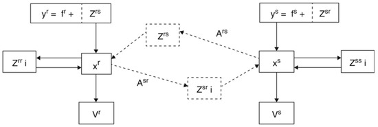
Figure 1.
Industry and regional interdependencies in an interregional input–output model. Source: Oosterhaven and Hewings, 2015.
Furthermore, by pre-multiplying the direct impact by the Leontief matrix, we obtain an estimation of the direct effects plus the indirect effects on the economic system, such as:
Therefore, when the gross output flows associated with a given level of final demand are known, relative changes in regional output can be assessed. Regional Brazilian economic hierarchies can thus be revealed as follows, considering a representative region R:
where is the vector of the gross output of R, is the Leontief inverse of this region, and is its change in final demand, accounted for by government transfers’ aggregate direct impact. It is important to consider that the results on gross output depend on interregional consumption preference structures, at least in the first round of income transfers. This aspect is particularly relevant in this study, because we assumed the same industrial household consumption structure so that demand increases in proportion to the amount received by households, and the consumption basket is maintained (preferences). The total value of the transfers received by each region was distributed proportionally to the sectors, following the distribution of household consumption present in the matrix.
3.1.2. Demand–Supply Combined Shocks
In the combined scenario, the demand shock as in scenario 1 is maintained, and supply constraints are also included from the hypothetical partial extraction [35]. The method is suitable for this empirical exercise, as it quantifies relative changes in total economic output with n sectors and r regions if a particular sector is partially contracted in this interregional system. The regional approach to the extraction method was first proposed by [36], and the full taxonomy can be found in [28]. The size of the intermediate consumption variations depends fundamentally on the level of essentiality of the economic activity. In this way, the entries of the technical coefficients matrix were altered according to the essentiality of each product (industry). Technical coefficients are thus multiplied by an essentiality index , ranging from 0 to 1. The closer to 1, the more essential the product can be considered. During the COVID-19 pandemic, industries were classified into different categories based on their level of essentiality within Brazil and Chile. This classification helped governments and public health authorities determine which businesses and services should remain open or receive priority during lockdowns and other restrictive measures. Following this setting, we have classified the IO industries of each country according to the degree of essentiality of each final good or service, encompassing three major levels: (1) essential; (2) mid-essential; (3) non-essential. In this regard, according to the final good or service, it would be possible to harmonize the different numbers of industries in each IRIO table.
It is important to note that the classification of essential industries varied from one jurisdiction to another, and it evolved as the pandemic situation changed. The goal was to balance the need to control the spread of the virus with the need to maintain essential services and support economic activity. For the empirical exercise proposed, we have followed the empirical literature on the essentiality of industries in order to classify the Brazilian and Chilean industries.
Therefore, the α values are similar to [37] and [35], implying a set of imbalances in the intermediate consumption matrix (called A matrix) within the IRIO economic system. The values of for each economic sector in Brazil and Chile are presented in Appendix C and Appendix D, respectively. Collectively, the simulation incorporates a partial reduction in the operating capacity of each sector, which affects interindustry relationships and, consequently, interregional dynamics. Therefore, the hypothetical matrix is given by:
Briefly, the models used in each scenario are as follows:
The variables’ dashes indicate the parts of the model where exogenous changes have been made according to the shocks applied.
3.2. Spatial Leakage Effects
Finally, to capture the regional absorption of the indirect effects of each shock in terms of the gross production value, the ratio between indirect and direct effects (RIDR) and the share of total indirect effects in each region (PIR) are used. These measurements indicate how much of the initial shock (direct effect) was absorbed in the region, and how much leaked to other regions. One can also interpret the leaks as wasted local revenue absorption potential, as given by:
Therefore, the calculated results allow us to quantify how much of the economic value of each region is transferred to other regions. Similarly, they can be interpreted as the extent to which a region misses out on relative gains.
4. Results
The maps in Figure 2 display the regional distribution of the indirect by direct effects ratio for the two shocks for Brazilian regional economy: (a) demand-only shock and (b) combined supply and demand shock. As expected, in the combined scenario, the magnitude of the effects is lower, indicating a greater reduction in the impact on regional output. However, disparities in the Brazilian economic geography lead the more prosperous economic areas to absorb the economic output regardless of the size of the simulated shock. Nevertheless, the regions that miss out the most are the peripheral ones, especially the smaller states economically and in terms of population, such as the northern states (Roraima and Amapá) and the northeastern states (such as Piauí and Paraíba). These peripheral states, despite receiving direct income transfers, fail to convert this increase in demand into local economic benefits. The spill-over effect benefits interregional production structures both directly and indirectly.
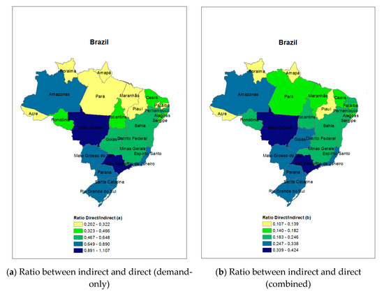
Figure 2.
RDI effects by Brazilian region. Panel (a) shows the regional distribution of RDI effects considering the demand-only scenario. Panel (b) shows the regional distribution of RDI effects for the combined demand and supply constraints scenario. (a) Ratio between indirect and direct effects (demand-only). (b) Ratio between indirect and direct effects (combined).
The maps in Figure 3 show the geographical distribution of RDI (Regional Demand Induced) effects for the Chilean regions. Similar to Brazil, in Chile, the effects spill over to the more prosperous economic areas, such as Antofagasta and the Metropolitan Region of Santiago. However, unlike Brazil, the spatial distribution of demand-only and combined effects in Chile is quite similar. This indicates that the structure of interregional transfers, despite being impacted, does not substantially alter the fact that the wealthy areas absorb shocks from both themselves and the poorer areas of the country.
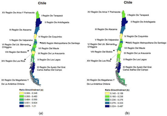
Figure 3.
RDI effects by Chilean region. Panel (a) shows the regional distribution of RDI effects considering the demand-only scenario. Panel (b) shows the regional distribution of RDI effects for the combined demand and supply constraints scenario. (a) Ratio between indirect and direct effects (demand-only). (b) Ratio between indirect and direct effects (combined).
In the Chilean case, unlike Brazil, the more diversified economic areas are in the Metropolitan Region of Santiago, where service activities and a significant portion of the national manufacturing industry are concentrated. The peripheral areas specialize in primary sectors, as seen in Antofagasta (northern) with mining activities and the southern regions specializing in agriculture. Consequently, the interregional structure of final demand tends to redistribute geographically, favouring the central areas.
Table 1 and Table 2 show the results for Brazil and Chile, respectively. In both tables, column one shows the list of regions analysed, columns two and three show the “indirect effects/direct effects” ratios in the demand shock (a) and the combined demand and supply shock (b), column four shows the ratio between these two shocks, and columns five and six show the share of each region in the indirect effects in the two shocks. These last two columns are used to analyse the results. Thus, it is not the value of the indirect effects but the share of each region in the total indirect effects generated in all regions that matters. It is considered that the increasing regional share of the total indirect effects is equivalent to reducing the leakage of income and employment to other regions.

Table 1.
Ratio between indirect and direct effects and Brazilian regions’ participation in the total indirect effects in the two simulated scenarios.
Table 2.
Ratio of indirect and direct effects and Chilean regions’ share in total indirect effects in the two simulated scenarios.
Table 1 shows Brazilian regions’ participation in the total indirect effects generated by the demand shock (household spending on Emergency Aid) and supply shock (supply constraints as an inverse function of essentiality). For the demand shock (column five), we see that the following have gained participation in the combined demand and supply shock (marked in grey): all the states in the north and northeast regions, which are the poorest in the country; and Minas Gerais, Mato Grosso, Mato Grosso do Sul, and Rio Grande do Sul, which are vital regions in agribusiness and agri-food chains. On the other hand, the states which lost relative participation were São Paulo and Rio de Janeiro, the main national economic centres, the Federal District, Espírito Santo, Paraná, and Santa Catarina.
These results show that the income leakage from the poorest and peripheral regions is relatively minor in the combined demand and supply shock (column 6) compared to the demand shock (column 5). Based on the inverse of product essentiality, supply shocks thus relatively favour the peripheral regions. One explanation for this is that essential products tend to have more geographically dispersed production, close to the supply of raw materials (high transportation costs, perishability). The traditional industrial location model from Weber shows us that sectors that “lose weight”, like agricultural-based industries, tend to locate themselves near raw materials suppliers. An example of this is agriculture and cattle raising. There is, therefore, a greater possibility of local supply in these sectors. Non-essential products, on the other hand, are produced mainly in large urban agglomerations.
The demand shock stems from household spending on government transfers (Emergency Aid), which includes purchasing various essential and non-essential products. In the supply shock, however, there is selectivity in favour of essential products. This is why, compared to the demand shock, the combined demand and supply shock results tend to cause less income leakage from the peripheral to the central regions.
Table 2 shows the Chilean regions’ results. Considering the last two columns, most regions gained relative participation in the indirect effects of the combined demand and supply shock compared to the demand shock. The regions that lost relative participation were the following (marked in grey): Metropolitan Santiago (RMS); Antofagasta (II); Atacama (III); Aysén del General Carlos Ibáñez del Campo (XI); and Magallanes y de la Antártica Chilena (XII).
The results represent the effect of geographic location and population density on the indirect supply constraint effects. These effects align with previous studies that address the degree of territorial vulnerability to events or threats of exogenous origin (e.g., [38]). For example, the regions of Antofagasta and Atacama (II and III, respectively), along with Aysén del General Carlos Ibáñez del Campo (XI) and Magallanes y de la Antártica Chilena (XII), are located in the far reaches of the country and are essential mineral and hydrocarbon producing areas. While regions II and III are in northern Chile, where a desert climate predominates, regions XI and XII are located in the extreme south of Chile, where a cold temperate climate and strong winds predominate year-round.
In these regions, the most significant economic effect is explained by the decline and volatility of mineral (mainly copper) and hydrocarbon prices, which unfortunately synchronized with the sharper period of economic inactivity in the spring of 2020. Along with the above, both groups of regions are distant from the main industrial centres of Chile, and their proportion of the economically active population is lower than the regions in the central zone of the country. In this sense, [3] recognizes two factors that condition territories’ vulnerability. First, there is their degree of exposure to risk situations beyond their control which cause insecurity. It is evident that when faced with a pandemic event, the outermost areas of the country receive some delay in the economic activation measures or the benefits of the health policies designed by the central government. Aspects such as logistical complexity, infrastructure, and accessibility could explain this situation. Second, there is the limited response capacity resulting from its internal weaknesses (derived from resource scarcity) and the lack of external support to mitigate the damage caused by the pandemic at the regional level.
In the case of the Metropolitan Region, there is a phenomenon associated with its excessive productive specialization and its economic profile linked to international value chains. In the first case, the loss of relative participation would be explained by the unfavourable performance of its productive sectors, mainly by unemployment among companies in branches considered non-priority. In the second case, the difficulty of generating effective integration to global value chains or external users also explains its recessive behaviour. The latter relates to several countries’ financial and logistical restrictions, limiting the international exchange of goods and services.
5. Conclusions and Policy Implications
This study compared two types of economic shocks during the COVID-19 pandemic to assess differences in income leakage between peripheral to central regions in Brazil and Chile. Regional absorptive capacity depends on economic conditions in subnational territories for the successful absorption of resource transfers (demand shock) and the reduction in leakages in the presence of supply shocks. However, in the presence of combined shocks, the potential for an increase in regional disparities within Brazil and Chile has become evident. The results of this study suggest that the absorptive capacity depends fundamentally on local production structures, the concentration of economic activity, local productive diversification, institutional aspects, and installed infrastructure. As a result, regional income transfers are converted into consumption. This generates indirect effects, which tend to propagate towards central areas via subnational chains, which are usually the most prosperous ones.
Overall, the results indicate that peripheral and less developed regions have a higher relative internal absorptive capacity for indirect effects when the shock is a combined supply and demand shock, compared to a demand-only shock. The main explanation for this result is that the supply restriction policy has had relatively less reach in the essential sectors, which are generally more dispersed geographically. In this way, the regions can retain more indirect effects, reducing leakage. Non-essential products, on the other hand, are generally produced with more spatial concentration and in large urban agglomerations. Local income retention is thus lower in the demand shock. In other words, a good part of interregional income leakage occurs because of non-essential product purchases by households.
Our empirical application has enabled us to analyse the relative importance of a region, which depends fundamentally on its set of economic activities and its relations with the rest of the economy [39]. This helps provide relevant ex ante perspectives on the systemic impact of economic policy shocks on regional economies at the sectoral level [40].
During the pandemic, there were transportation difficulties as well, which reduced interregional trade flow between regions. This also benefited local providers by increasing the absorption of indirect effects, though. There may have subsequently been an increase in regional import substitution, increasing the consumption of products offered by local companies, especially essential products. As explained earlier, this is feasible because the production of essential products tends to be relatively more dispersed in geographic space than that of non-essential products. However, in the long run, restrictions on interregional trade, as occurred during the pandemic, are also expected to cause the further spatial deconcentration of economic activities. According to the teachings of the New Economic Geography, the increase in transportation costs (increased barriers to trade) tends to stimulate industrial deconcentration as well.
Despite the results of this study indicating that income absorption by the poorest regions is relatively higher in the case of a supply shock, it can be asserted that this type of shock enhances the retention of income generated in these economically disadvantaged areas, thereby fostering local development and reducing regional inequalities. However, as this study relies on a structural input–output model, the analytical scope of the findings is directly related to the degree of linkage between sectors and regions. In other words, while the results allow us to determine the spatial direction of leakages, they do not necessarily provide the precise value of interregional leakage. This is because the model incorporates the entire set of structural relationships among regions and sectors within a country, which can potentially overestimate some of the outcomes.
Finally, these results can be essential for public policy formulation. For example, suppose the objective is to deconcentrate economic activity spatially or promote peripheral regions’ development. In that case, a potentially promising path is to encourage or attract companies based on the criterion of their products’ essentiality. Furthermore, the technique adopted can be extended to evaluate different resource transfer strategies to reduce regional disparities, where hierarchies can be defined regarding activities produced that can potentially increase local absorptive capacity.
Author Contributions
Conceptualization, A.F. and E.R.S.; methodology, A.F.; software, E.R.S.; validation, P.B., R.V., and A.F.; formal analysis, A.F.; investigation, A.F.; resources, E.R.S.; data curation, E.R.S.; writing—original draft preparation, A.F.; writing—review and editing, A.F. and E.R.S.; supervision, A.F.; project administration, E.R.S.; funding acquisition, E.R.S. All authors have read and agreed to the published version of the manuscript.
Funding
This research was funded by AGENCIA NACIONAL DE INVESTIGACIÓN Y DESARROLLO (ANID), grant number ANID-FOVI-210046.
Data Availability Statement
Not applicable.
Acknowledgments
The authors thank the Regional and Urban Economics Lab (NEREUS) at the University of Sao Paulo (USP) for providing the input–output tables used in this study.
Conflicts of Interest
The authors declare no conflict of interest.
Appendix A
Table A1.
Direct and indirect effects in Brazilian regions (BRL million).
Table A1.
Direct and indirect effects in Brazilian regions (BRL million).
| Brazilian Region | Direct Effect * | Indirect Effect | Total Effect | Indirect Effect | Total Effect |
|---|---|---|---|---|---|
| (a) | (a) | (a) | (b) | (b) | |
| RR | 1255.30 | 256.49 | 1511.79 | 134.12 | 1389.42 |
| AP | 1893.50 | 382.52 | 2276.02 | 218.22 | 2111.72 |
| AC | 1820.90 | 479.24 | 2300.14 | 251.96 | 2072.86 |
| PI | 7034.00 | 1990.29 | 9024.29 | 977.35 | 8011.35 |
| PB | 8480.00 | 2699.27 | 11,179.27 | 1299.19 | 9779.19 |
| PA | 18,310.00 | 5801.37 | 24,111.37 | 2856.80 | 21,166.80 |
| MA | 14,985.00 | 4827.77 | 19,812.77 | 2379.33 | 17,364.33 |
| AL | 7188.00 | 2711.00 | 9899.00 | 1249.12 | 8437.12 |
| CE | 19,478.00 | 7715.15 | 27,193.15 | 3553.84 | 23,031.84 |
| RN | 6918.00 | 3222.70 | 10,140.70 | 1378.49 | 8296.49 |
| SE | 4843.00 | 2247.63 | 7090.63 | 1009.50 | 5852.50 |
| TO | 2889.10 | 1292.70 | 4181.80 | 630.21 | 3519.31 |
| BA | 32,490.00 | 17,343.55 | 49,833.55 | 7224.72 | 39,714.72 |
| PE | 20,982.00 | 11,046.31 | 32,028.31 | 4921.48 | 25,903.48 |
| RO | 3293.40 | 1471.08 | 4764.48 | 802.47 | 4095.87 |
| MG | 33,859.00 | 20,231.21 | 54,090.21 | 8335.50 | 42,194.50 |
| GO | 12,254.00 | 7937.75 | 20,191.75 | 3426.33 | 15,680.33 |
| ES | 6677.00 | 5257.87 | 11,934.87 | 1952.73 | 8629.73 |
| DF | 4253.20 | 3180.12 | 7433.32 | 1265.41 | 5518.61 |
| AM | 8611.00 | 6440.11 | 15,051.11 | 2653.28 | 11,264.28 |
| RJ | 30,081.00 | 26,763.11 | 56,844.11 | 9307.57 | 39,388.57 |
| MS | 4910.70 | 3579.51 | 8490.21 | 1566.18 | 6476.88 |
| RS | 15,174.00 | 12,578.67 | 27,752.67 | 5038.74 | 20,212.74 |
| SC | 8422.80 | 7164.32 | 15,587.12 | 2816.85 | 11,239.65 |
| PR | 16,809.00 | 14,424.02 | 31,233.02 | 5686.85 | 22,495.85 |
| SP | 66,410.00 | 73,532.08 | 139,942.08 | 26,410.22 | 92,820.22 |
| MT | 6187.00 | 6182.20 | 12,369.20 | 2625.91 | 8812.91 |
| Total | 365,508.90 | 250,758.04 | 616,266.94 | 99,972.36 | 465,481.26 |
Notes: (*) direct effect corresponds to the value of government transfers to regions in the pandemic; (a) without supply constraint; (b) with supply constraint; RR = Roraima; AP = Amapá; AC = Acre; PI = Piauí; PB = Paraíba; PA = Pará; MA = Maranhão; AL = Alagoas; CE = Ceará; RN = Rio Grande do Norte; SE = Sergipe; TO = Tocantins; BA = Bahia; PE = Pernambuco; RO = Rondônia; MG = Minas Gerais; GO = Goiás; ES = Espírito Santo; DF = Distrito Federal; AM = Amazonas; RJ = Rio de Janeiro; MS = Mato Grosso do Sul; RS = Rio Grande do Sul; SC = Santa Catarina; PR = Paraná; SP = São Paulo; MT = Mato Grosso.
Appendix B
Table A2.
Direct and indirect effects in Chilean regions (Chilean Pesos).
Table A2.
Direct and indirect effects in Chilean regions (Chilean Pesos).
| Chilean Region | Direct Effect * | Indirect Effect | Total Effect | Indirect Effect | Total Effect |
|---|---|---|---|---|---|
| (a) | (a) | (a) | (b) | (b) | |
| RMS | 1013.01 | 835.13 | 1848.13 | 327.11 | 1340.12 |
| VIII | 370.81 | 204.01 | 574.81 | 94.06 | 464.86 |
| V | 304.72 | 164.87 | 469.59 | 71.7 | 376.42 |
| IX | 222.73 | 68.26 | 290.99 | 31.19 | 253.92 |
| VII | 215.45 | 96.17 | 311.62 | 47.47 | 262.91 |
| X | 169.16 | 86 | 255.16 | 37.45 | 206.61 |
| VI | 168.43 | 88.82 | 257.25 | 37.62 | 206.05 |
| IV | 140.19 | 48.86 | 189.05 | 22.22 | 162.41 |
| XIV | 79.34 | 37.72 | 117.06 | 16.8 | 96.14 |
| II | 75.02 | 90.72 | 165.74 | 36.56 | 111.58 |
| I | 55.59 | 26.84 | 82.43 | 11.49 | 67.08 |
| III | 53.37 | 35.54 | 88.91 | 16.31 | 69.68 |
| XV | 44.57 | 19.65 | 64.22 | 8.94 | 53.5 |
| XII | 20.44 | 13.82 | 34.26 | 5.63 | 26.07 |
| XI | 18.49 | 17.9 | 36.39 | 7.64 | 26.13 |
| Total | 2951.31 | 1834.32 | 4785.63 | 772.18 | 3723.50 |
Notes: (*) the direct effect corresponds to the value of government transfers to the regions in the pandemic; (a) without supply restriction; (b) with supply restriction; RMS = Región Metropolitana de Santiago; VIII = Del Biobío; V = De Valparaíso; IX = De La Araucanía; VII = Del Maule; X = De Los Lagos; VI = Del Libertador General Bernardo O’Higgins; IV = De Coquimbo; XIV = De Los Ríos; II = De Antofagasta; I = De Tarapacá; III = De Atacama; XV = De Arica y Parinacota; XII = De Magallanes y de la Antártica Chilena; XI = Aysén del General Carlos Ibáñez del Campo.
Appendix C
Table A3.
Sector classification by essentiality—Brazil.
Table A3.
Sector classification by essentiality—Brazil.
| Sector ID | Sectors | Essentiality | Alpha |
|---|---|---|---|
| S1 | Agriculture, including agricultural and post-harvest support | Essential | 1.0 |
| S2 | Livestock, including support for livestock | Essential | 1.0 |
| S3 | Forestry production; fishing and aquaculture | Essential | 1.0 |
| S4 | Coal and non-metallic minerals extraction | Mid-essential | 0.7 |
| S5 | Oil and gas extraction, including support activities | Mid-essential | 0.7 |
| S6 | Iron ore extraction, including beneficiation and agglomeration | Mid-essential | 0.7 |
| S7 | Non-ferrous metallic minerals extraction, including beneficiation | Mid-essential | 0.7 |
| S8 | Slaughtering and meat products, including dairy and fishery products | Mid-essential | 0.7 |
| S9 | Sugar manufacturing and refining | Non-essential | 0.5 |
| S10 | Other food products | Non-essential | 0.5 |
| S11 | Beverage manufacturing | Non-essential | 0.5 |
| S12 | Tobacco products manufacturing | Non-essential | 0.5 |
| S13 | Textile manufacturing | Non-essential | 0.5 |
| S14 | Manufacture of clothing apparel and accessories | Non-essential | 0.5 |
| S15 | Footwear and leather goods manufacturing | Non-essential | 0.5 |
| S16 | Wood products manufacturing | Non-essential | 0.5 |
| S17 | Pulp and paper manufacturing | Non-essential | 0.5 |
| S18 | Printing and reproduction of recorded media | Non-essential | 0.5 |
| S19 | Oil refining and coking | Non-essential | 0.5 |
| S20 | Biofuel manufacturing | Non-essential | 0.5 |
| S21 | Organic and inorganic chemicals, resins, and elastomers manufacturing | Non-essential | 0.5 |
| S22 | Manufacture of pesticides, disinfectants, paints, and various chemicals | Non-essential | 0.5 |
| S23 | Cleaning, cosmetics/perfumery, and personal care products manufacturing | Non-essential | 0.5 |
| S24 | Pharmochemical and pharmaceutical products manufacturing | Non-essential | 0.5 |
| S25 | Rubber and plastic products manufacturing | Non-essential | 0.5 |
| S26 | Non-metallic mineral products manufacturing | Non-essential | 0.5 |
| S27 | Production of pig iron/ferroalloys, steelmaking, and seamless steel tubes | Non-essential | 0.5 |
| S28 | Non-ferrous metal metallurgy and metal casting | Non-essential | 0.5 |
| S29 | Metal products manufacturing, except machinery and equipment | Non-essential | 0.5 |
| S30 | Manufacturing of computer, electronic, and optical products | Non-essential | 0.5 |
| S31 | Electrical machinery and equipment manufacturing | Non-essential | 0.5 |
| S32 | Machinery and mechanical equipment manufacturing | Non-essential | 0.5 |
| S33 | Automotive, trucks, and buses manufacturing, except parts | Non-essential | 0.5 |
| S34 | Automotive parts and accessories manufacturing | Non-essential | 0.5 |
| S35 | Manufacture of other transport equipment, except motor vehicles | Non-essential | 0.5 |
| S36 | Furniture and miscellaneous industrial manufacturing | Non-essential | 0.5 |
| S37 | Maintenance, repair, and installation of machinery and equipment | Non-essential | 0.5 |
| S38 | Electricity, natural gas, and other utilities | Essential | 1.0 |
| S39 | Water, sewage, and waste management | Essential | 1.0 |
| S40 | Construction | Non-essential | 0.5 |
| S41 | Wholesale and retail | Non-essential | 0.5 |
| S42 | Land transport | Mid-essential | 0.7 |
| S43 | Waterborne transport | Essential | 1.0 |
| S44 | Aviation | Mid-essential | 0.7 |
| S45 | Storage, auxiliary transport activities, and postal services | Mid-essential | 0.7 |
| S46 | Accommodation | Non-essential | 0.5 |
| S47 | Food | Non-essential | 0.5 |
| S48 | Print-integrated editing and editing | Non-essential | 0.5 |
| S49 | Television, radio, film, and sound and image recording/editing activities | Non-essential | 0.5 |
| S50 | Telecommunications | Mid-essential | 0.7 |
| S51 | System development and other information services | Non-essential | 0.5 |
| S52 | Financial intermediation, insurance, and complementary pension plans | Non-essential | 0.5 |
| S53 | Real estate activities | Non-essential | 0.5 |
| S54 | Legal, accounting, consulting, and corporate headquarters activities | Non-essential | 0.5 |
| S55 | Architectural, engineering, technical testing/analysis, and R&D services | Non-essential | 0.5 |
| S56 | Other professional, scientific, and technical activities | Non-essential | 0.5 |
| S57 | Non-Real Estate Rentals and Intellectual Property Asset Management | Non-essential | 0.5 |
| S58 | Other administrative activities and complementary services | Non-essential | 0.5 |
| S59 | Surveillance, security, and investigation activities | Non-essential | 0.5 |
| S60 | Public administration, defence, and social security | Non-essential | 0.5 |
| S61 | Public Education | Mid-essential | 0.7 |
| S62 | Private Education | Mid-essential | 0.7 |
| S63 | Public healthcare | Mid-essential | 0.7 |
| S64 | Private healthcare | Essential | 1.0 |
| S65 | Artistic, creative, and performing activities | Essential | 1.0 |
| S66 | Membership organizations and other personal services | Non-essential | 0.5 |
| S67 | Housekeeping services | Non-essential | 0.5 |
Appendix D
Table A4.
Sector classification by essentiality—Chile.
Table A4.
Sector classification by essentiality—Chile.
| Sector ID | Sectors | Essentiality | Alpha |
|---|---|---|---|
| S1 | Agriculture, Forestry, and Fishing | Essential | 1.0 |
| S2 | Mining | Mid-essential | 0.7 |
| S3 | Manufacturing industry | Non-essential | 0.5 |
| S4 | Electricity, gas, water, and waste management | Essential | 1.0 |
| S5 | Construction | Non-essential | 0.5 |
| S6 | Retail, hotels, and restaurants | Non-essential | 0.5 |
| S7 | Transportation, communications, and information services | Mid-essential | 0.7 |
| S8 | Financial intermediation | Non-essential | 0.5 |
| S9 | Real estate and housing services | Non-essential | 0.5 |
| S10 | Business services | Non-essential | 0.5 |
| S11 | Personal services | Non-essential | 0.5 |
| S12 | Public administration | Essential | 1.0 |
References
- Esquivel, G. Pandemia, confinamiento y crisis: ¿Qué hacer para reducir los costos económicos y sociales? Descarga Responsab. 2020, 134–141. [Google Scholar] [CrossRef]
- Lavell, A.; Mansilla, E.; Maskrey, A.; Ramirez, F. The Social Construction of the COVID-19 pandemic: Disaster, Risk Accumulation and Public Policy. Red de Estudios Sociales en Prevención de Desastres en América Latina (LA RED). 2020. Available online: https://www.desenredando.org/covid19/Construcci%C3%B3n-social-pandemia-Covid19-desastre-riesgo-politicas-publicas-RNI-LA-RED-23-04-2020.pdf (accessed on 15 October 2022).
- Méndez, R. Sitiados por la Pandemia. Apuntes Geográficos; Revives: Madrid, Spain, 2020. [Google Scholar]
- Haddad, E.A.; Perobelli, F.S.; Araújo, I.F.; Bugarin, K.S. Structural propagation of pandemic shocks: An input–output analysis of the economic costs of COVID-19. Spat. Econ. Anal. 2021, 16, 252–270. [Google Scholar] [CrossRef]
- Ferreira Moutinho, R.F. Absorptive capacity and business model innovation as rapid development strategies for regional growth. Investig. Económica 2016, 75, 157–202. [Google Scholar] [CrossRef]
- Crescenzi, R.; Giua, M. The EU Cohesion Policy in context: Regional growth and the influence of agricultural and rural development policies. LEQS Discussion Paper No. 85/2014. SSRN Electron. J. 2014. [Google Scholar] [CrossRef][Green Version]
- Incaltarau, C.; Pascariu, G.C.; Surubaru, N.C. Evaluating the Determinants of EU Funds Absorption across Old and New Member States—the Role of Administrative Capacity and Political Governance. J. Common Mark. Stud. 2020, 58, 941–961. [Google Scholar] [CrossRef]
- del Rio-Chanona, R.M.; Mealy, P.; Pichler, A.; Lafond, F.; Farmer, D. Supply and demand shocks in the COVID-19 pandemic: An industry and occupation perspective. Oxf. Rev. Econ. Policy 2020, 36, S94–S137. [Google Scholar] [CrossRef]
- Sajid, M.J.; Qingren, C.; Ming, C.; Shuang, L. Sectoral carbon linkages of Indian economy based on hypothetical extraction model. Int. J. Clim. Change Strateg. Manag. 2020, 12, 1756–8692. [Google Scholar] [CrossRef]
- Brinca, P.; Duarte, J.B.; Faria-e-Castro, M. Measuring labor supply and demand shocks during COVID-19. Eur. Econ. Rev. 2021, 139, 103901. [Google Scholar] [CrossRef]
- Sajid, M.J.; Gonzalez, E.D.R.S. The Impact of Direct and Indirect COVID-19 Related Demand Shocks on Sectoral CO2 Emissions: Evidence from Major Asia Pacific Countries. Sustainability 2021, 13, 9312. [Google Scholar] [CrossRef]
- Nassif Pires, L.; Carvalho, L.B.D.; Lederman Rawet, E. Multi-dimensional inequality and COVID-19 in Brazil. Investig. Económica 2021, 80, 33–58. [Google Scholar] [CrossRef]
- Krugman, P. Scale Economies, Product Differentiation, and the Pattern of Trade. Am. Econ. Rev. 1980, 70, 950–959. [Google Scholar]
- Leontief, W. Domestic Production and Foreign Trade: The American Capital Position Re-examined. Proc. Am. Philos. Soc. 1953, 97, 332–349. [Google Scholar]
- Isard, W. Location Theory and Regional Economic Growth. Q. J. Econ. 1954, 68, 305–322. [Google Scholar] [CrossRef]
- Avelino, A.F.; Dall’erba, S. Comparing the economic impact of natural disasters generated by different input–output models: An application to the 2007 Chehalis river flood (wa). Risk Anal. 2019, 39, 85–104. [Google Scholar] [CrossRef]
- Pichler, A.; Farmer, J.D. Simultaneous supply and demand constraints in input–output networks: The case of COVID-19 in Germany, Italy, and Spain. Econ. Syst. Res. 2022, 34, 273–293. [Google Scholar] [CrossRef]
- Menezes-Filho, N.; Komatsu, B.K.; Rosa, J.P. Reducing poverty and inequality during the Coronavirus outbreak: The emergency aid transfers in Brazil. Policy Paper n.54 2021. [Google Scholar]
- Organização Pan-Americana Da Saúde (OPAS). Saúde nas Américas 2022. In Panorama da Região das Américas no Contexto da Pandemia de COVID-19; Organização Pan-Americana Da Saúde: Washington, DC, USA, 2022. [Google Scholar]
- de Paula, L.F. The COVID-19 crisis and counter-cyclical policies in Brazil. Eur. J. Econ. Econ. Policies Interv. 2021, 18, 177–197. [Google Scholar] [CrossRef]
- Garcia, M.L.T.; Pandolfi, A.F.; Leal, F.X.; Stocco, A.F.; Borrego, A.E.; Borges, R.E.; Oliveira, E.F.D.A.; Lang, A.E.; Andrade, C.O. The COVID-19 pandemic, emergency aid and social work in Brazil. Qual. Soc. Work. 2021, 20, 356–365. [Google Scholar] [CrossRef]
- Silva, L.L.S.D.; Lima, A.F.R.; Polli, D.A.; Razia, P.F.S.; Pavão, L.F.A.; Cavalcanti, M.A.F.D.H.; Toscano, C.M. Medidas de distanciamento social para o enfrentamento da COVID-19 no Brasil: Caracterização e análise epidemiológica por estado. Cad. Saúde Pública 2020, 36. [Google Scholar] [CrossRef]
- Eichenbaum, M.S.; Rebelo, S.; Trabandt, M. The macroeconomics of epidemics. Rev. Financ. Stud. 2021, 34, 5149–5187. [Google Scholar] [CrossRef]
- Cardoso, B.B. A implementação do Auxílio Emergencial como medida excepcional de proteção social. Rev. Adm. Pública 2020, 54, 1052–1063. [Google Scholar] [CrossRef]
- Comissão Econômica para América Latina e o Caribe. Cepalstat: Principales Cifras de América Latina y el Caribe; CEPAL: Santiago, Chile, 2022; Available online: https://statistics.cepal.org/portal/cepalstat/index.html?lang=es (accessed on 15 October 2022).
- Trovão, C.J.B.M. A Pandemia da COVID-19 e a Desigualdade de Renda no Brasil: Um Olhar Macrorregional Para a Proteção Social e os Auxílios Emergenciais; Universidade Federal do Rio Grande do Norte: Natal, Brazil, 2020. [Google Scholar]
- da Rosa, P.R.; Fochezatto, A.; Neto, G.B.; Sanguinet, E.R. Social protection and COVID-19: Evaluation of regional impacts of the Emergency Aid policy in Brazil. EconomiA 2021, 22, 239–250. [Google Scholar] [CrossRef]
- Haddad, E.A.; Júnior, C.A.G.; Nascimento, T.O. Matriz interestadual de insumo-produto para o Brasil: Uma aplicação do método IIOAS. Rev. Bras. Estud. Reg. E Urbanos 2017, 11, 424–446. [Google Scholar]
- Kersan Škabić, I.; Tijanić, L. Regional abrorption capacity of EU funds. Econ. Res.-Ekon. Istraživanja 2017, 30, 1192–1208. [Google Scholar] [CrossRef]
- Caragliu, A.; Nijkamp, P. The impact of regional absorptive capacity on spatial knowledge spillovers: The Cohen and Levinthal model revisited. Appl. Econ. 2012, 44, 1363–1374. [Google Scholar] [CrossRef]
- Apostolopoulos, N.; Liargovas, P.; Rodousakis, N.; Soklis, G. COVID-19 in US Economy: Structural Analysis and Policy Proposals. Sustainability 2022, 14, 7925. [Google Scholar] [CrossRef]
- Cace, C.; Cace, S.; Iova, C.; Nicolaescu, V. Absorption capacity of the structural funds. Integrating perspectives. Rev. Cercet. Interv. Soc. 2009, 27, 7–28. [Google Scholar]
- Ferreira, F.H.; Gignoux, J. The measurement of inequality of opportunity: Theory and an application to Latin America. Rev. Income Wealth 2011, 57, 622–657. [Google Scholar] [CrossRef]
- López, R.; Thomas, V. Closing Gaps in Regional Disparities in Chile. World Bank Policy Res. Work. Pap. 2014, 6877. [Google Scholar]
- Timmer, M.; Los, B.; Stehrer, R.; De Vries, G. An Anatomy of the Global Trade Slowdown Based on the WIOD 2016 Release; GGDC Research Memorandum GD-162; Groningen Growth and Development Centre, University of Groningen: Groningen, The Netherlands, 2016; pp. 1–65. Available online: https://ideas.repec.org/p/gro/rugggd/gd-162.html (accessed on 15 October 2022).
- Sanguinet, E.R.; Alvim, A.M.; Atienza, M.; Fochezatto, A. The subnational supply chain and the COVID-19 pandemic: Short-term impacts on the Brazilian regional economy. Reg. Sci. Policy Pract. 2021, 13, 158–186. [Google Scholar] [CrossRef]
- Dietzenbacher, E.; Linden, J.; Steenge, A. The regional extraction method: EC input–output comparisons. Econ. Syst. Res. 1993, 5, 185–206. [Google Scholar] [CrossRef]
- Bonet-Morón, J.; Ricciulli-Marín, D.; Pérez-Valbuena, G.J.; Galvis-Aponte, L.A.; Haddad, E.A.; Araújo, I.F.; Perobelli, F.S. Impacto económico regional del Covid-19 en Colombia: Un análisis insumo-producto. Banco República 2020, 288, 34. [Google Scholar]
- Wilches-Chaux, G. La vulnerabilidad global. In Los Desastres No Son Naturales; Centro de Estudios del Hábitat Popular, Universidad Nacional de Colombia: Medellin, Colombia, 1993; pp. 11–44. [Google Scholar]
- Miller, R.; Blair, P. Input-Output Analysis: Foundations and Extensions; Cambridge University Press: Cambridge, UK, 2009. [Google Scholar]
Disclaimer/Publisher’s Note: The statements, opinions and data contained in all publications are solely those of the individual author(s) and contributor(s) and not of MDPI and/or the editor(s). MDPI and/or the editor(s) disclaim responsibility for any injury to people or property resulting from any ideas, methods, instructions or products referred to in the content. |
© 2023 by the authors. Licensee MDPI, Basel, Switzerland. This article is an open access article distributed under the terms and conditions of the Creative Commons Attribution (CC BY) license (https://creativecommons.org/licenses/by/4.0/).