
Spatiotemporal Variation of Summertime Urban Heat Island (UHI) and Its Correlation with Particulate Matter (PM2.5) over Metropolitan Cities in Alabama


Abstract
:1. Introduction
2. Data and Methodology
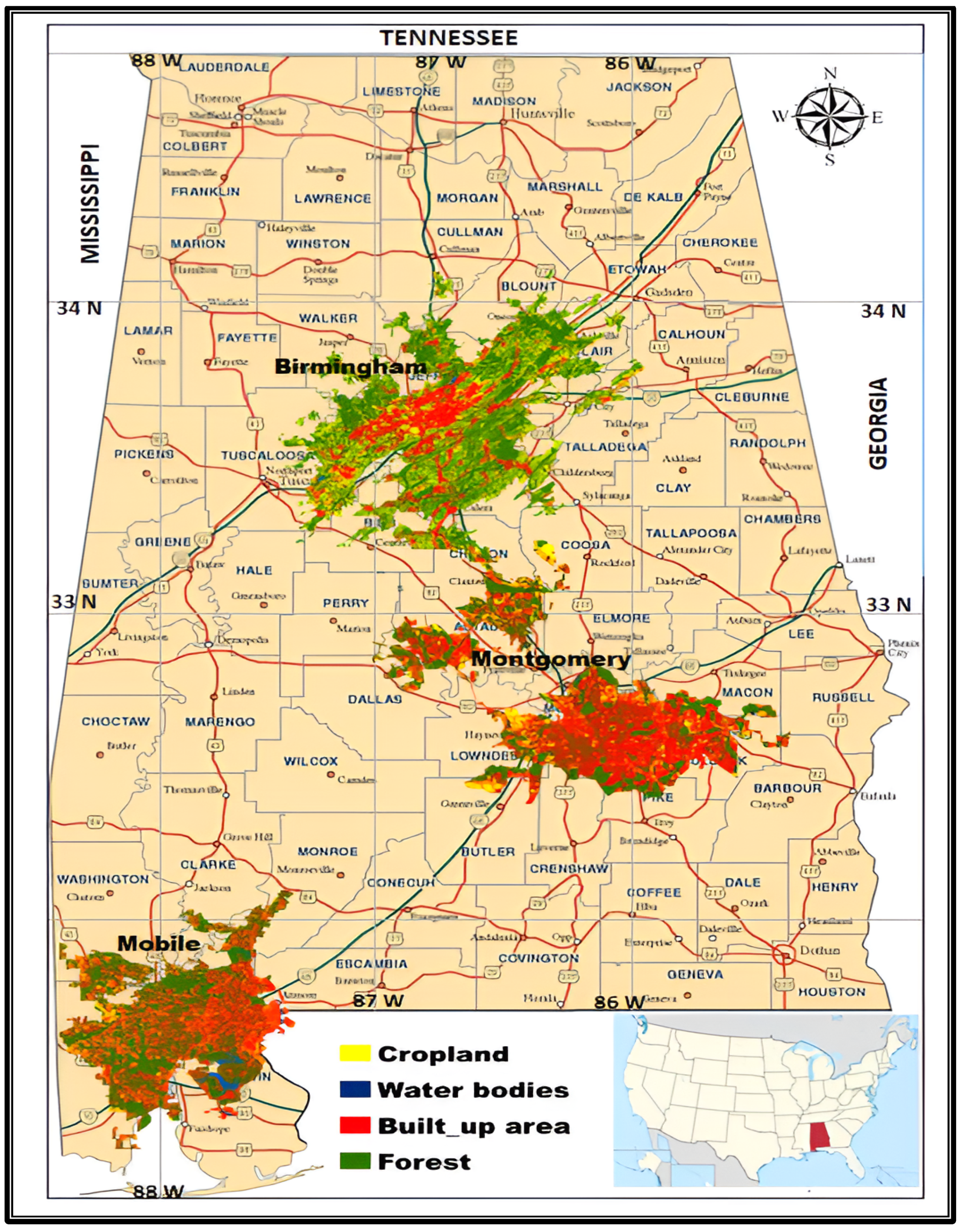
2.1. Description of the Study Area
2.2. Data
2.2.1. Land Surface Temperature (LST) Data
2.2.2. Fine Particulate Matter (PM2.5) Data
2.3. Methods
2.3.1. LULC Classification Technique
2.3.2. Images Preprocessing
2.3.3. UHI Calculation
2.3.4. NDBI Calculation
2.3.5. PM2.5 Spatial Interpolation Model
3. Results
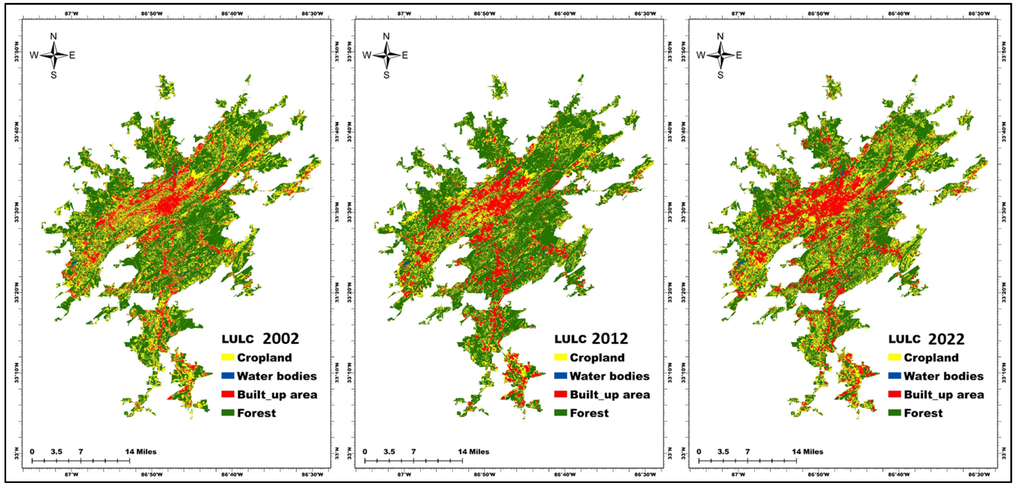
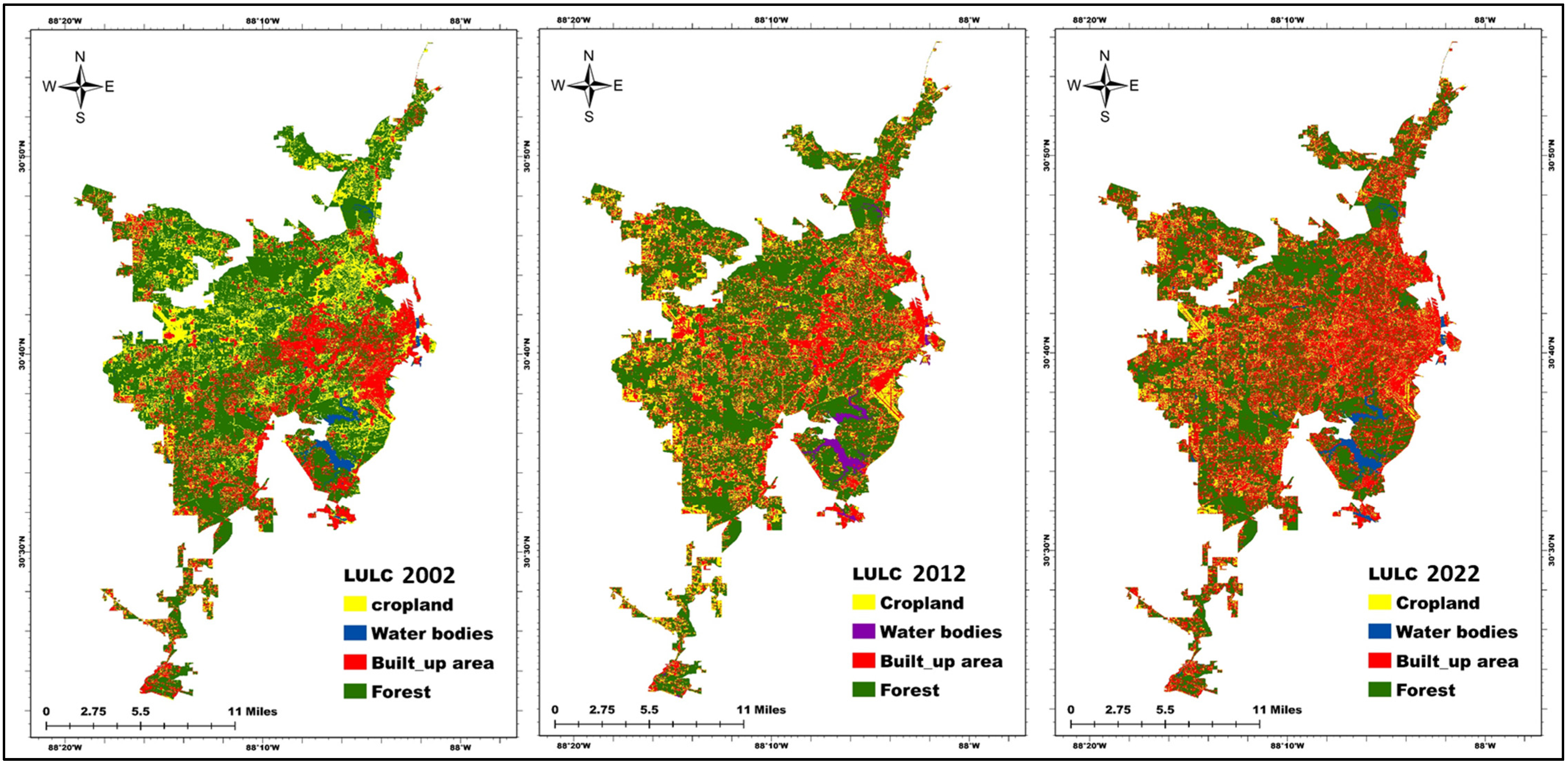
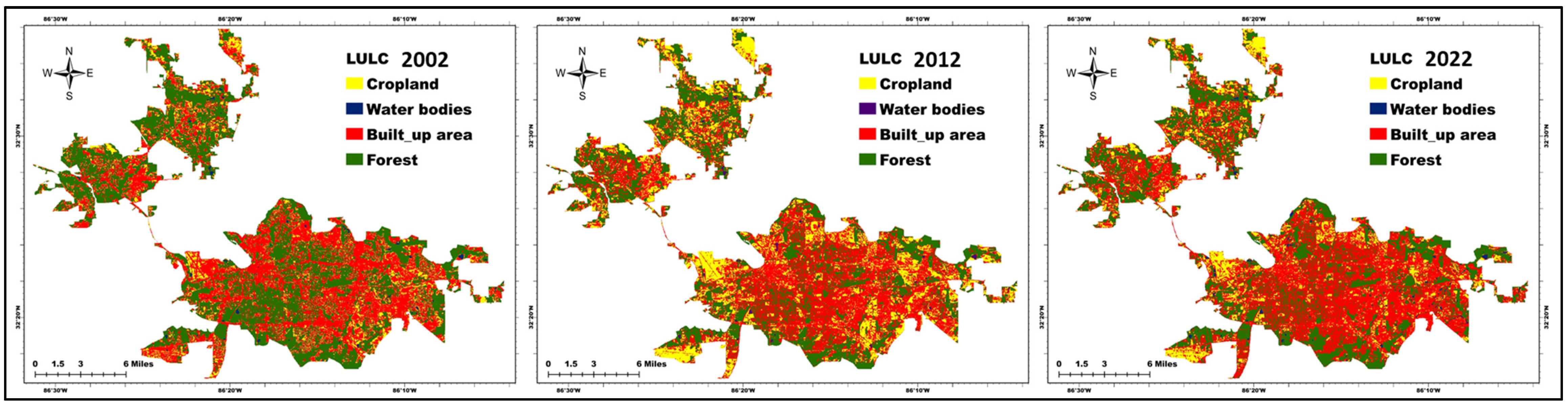
3.1. LULC Changes
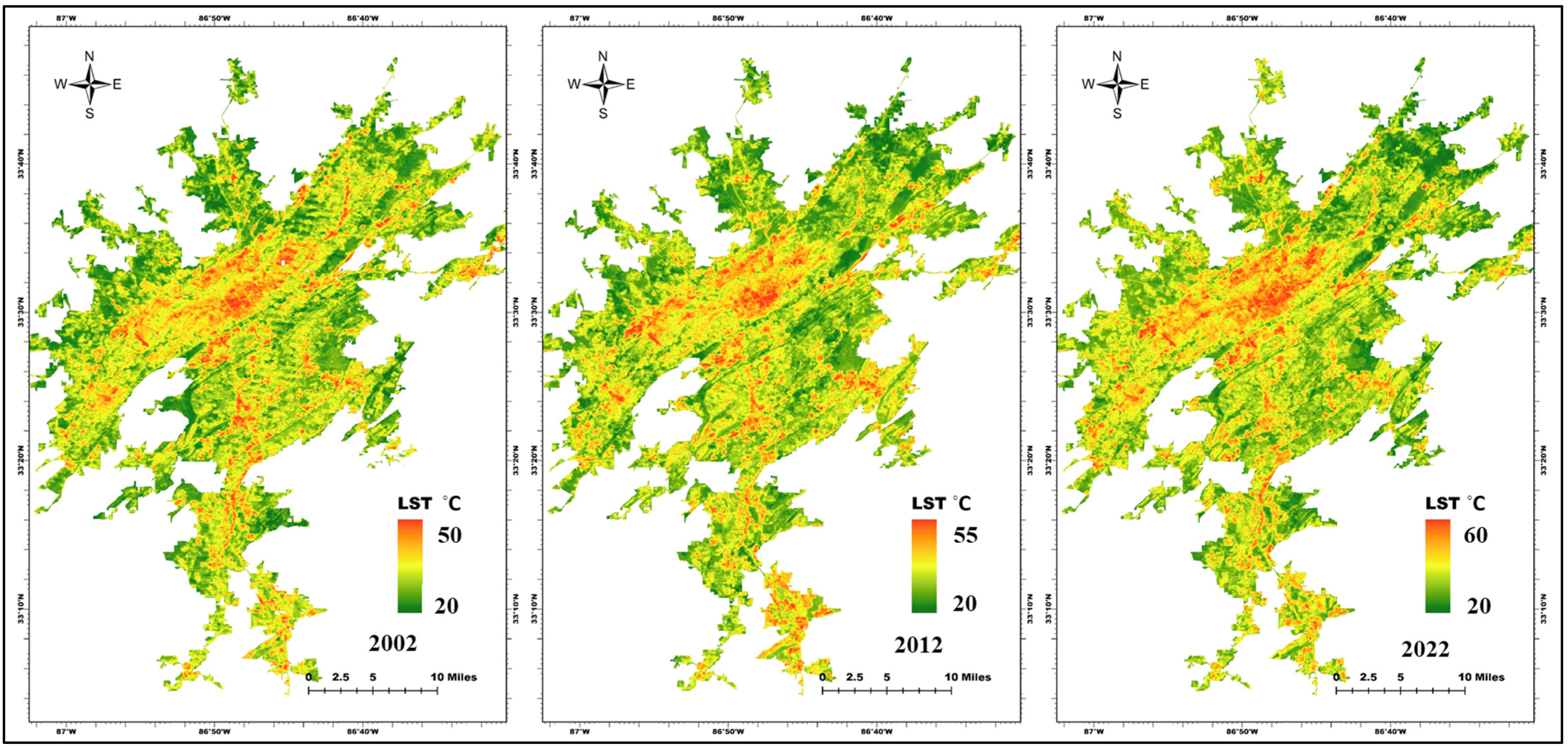
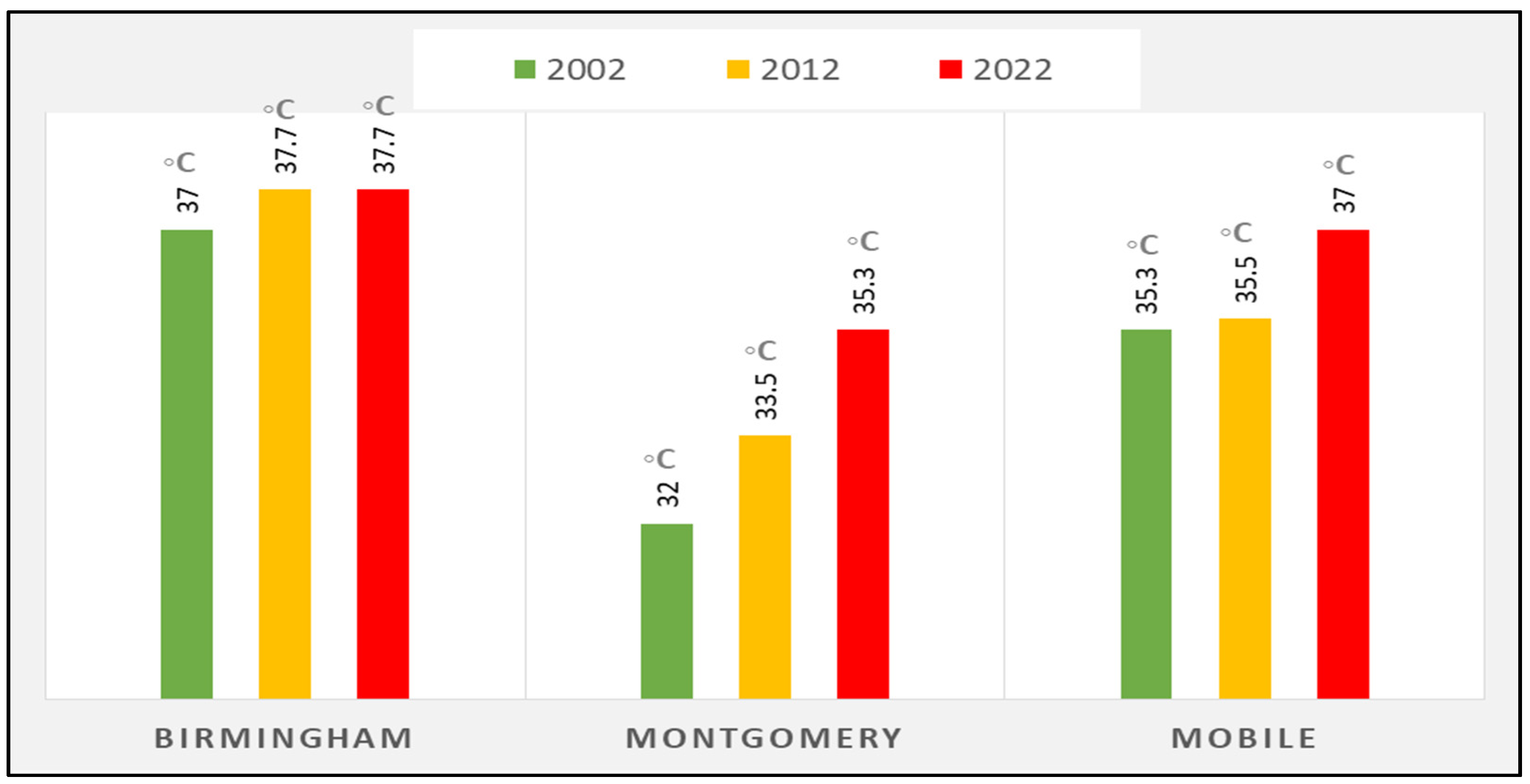
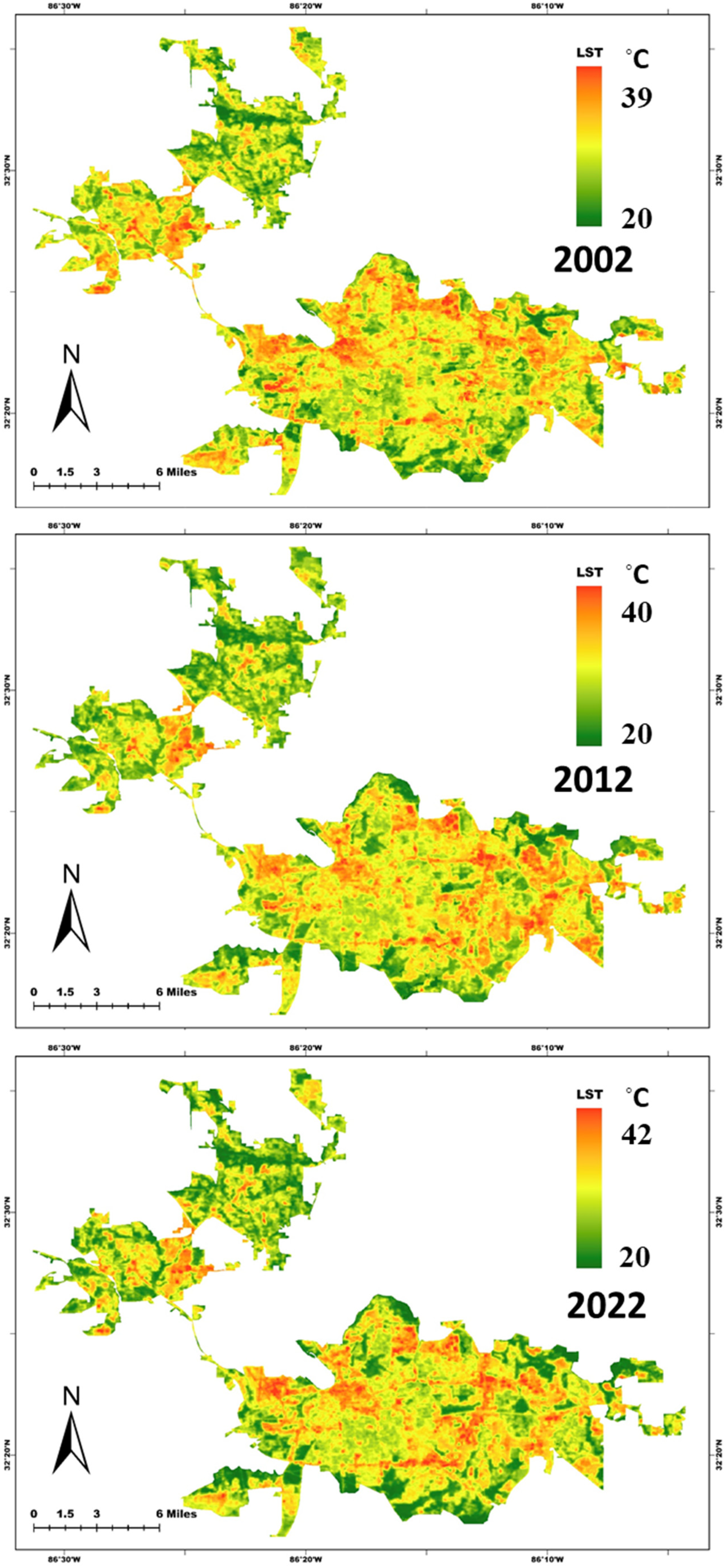
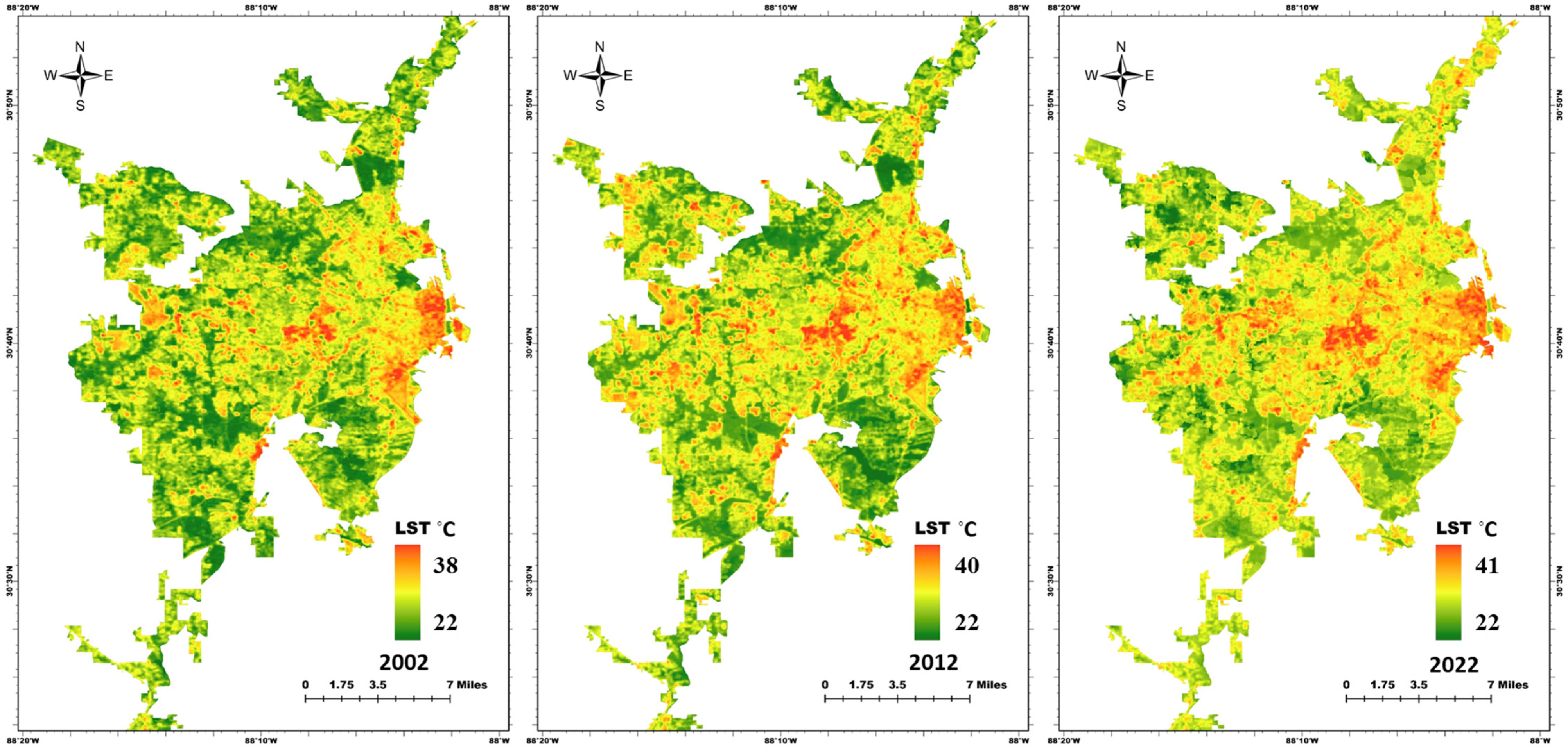
3.2. Spatiotemporal Variations of LST
3.3. Effects of LULC Change on UHI
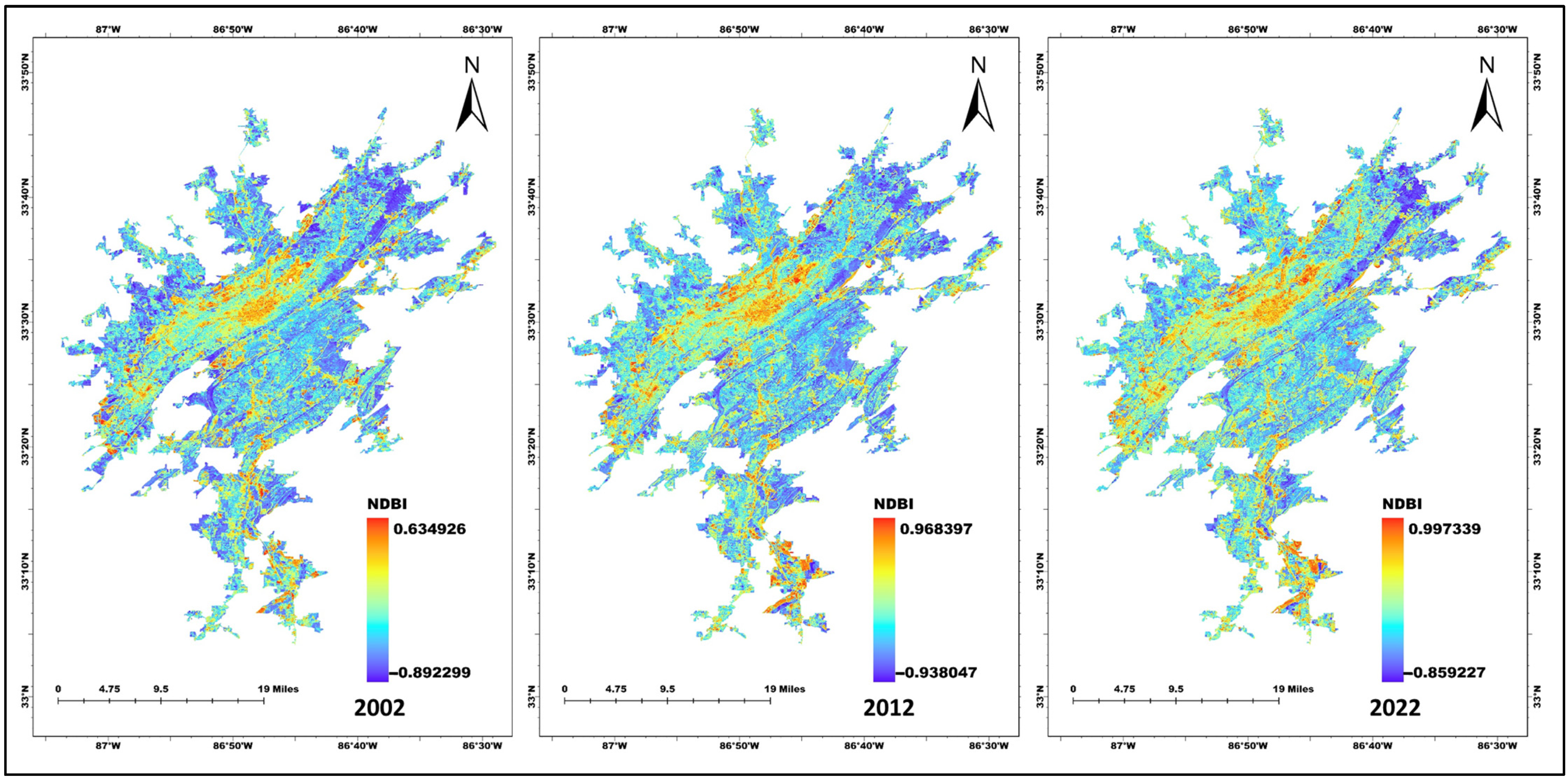
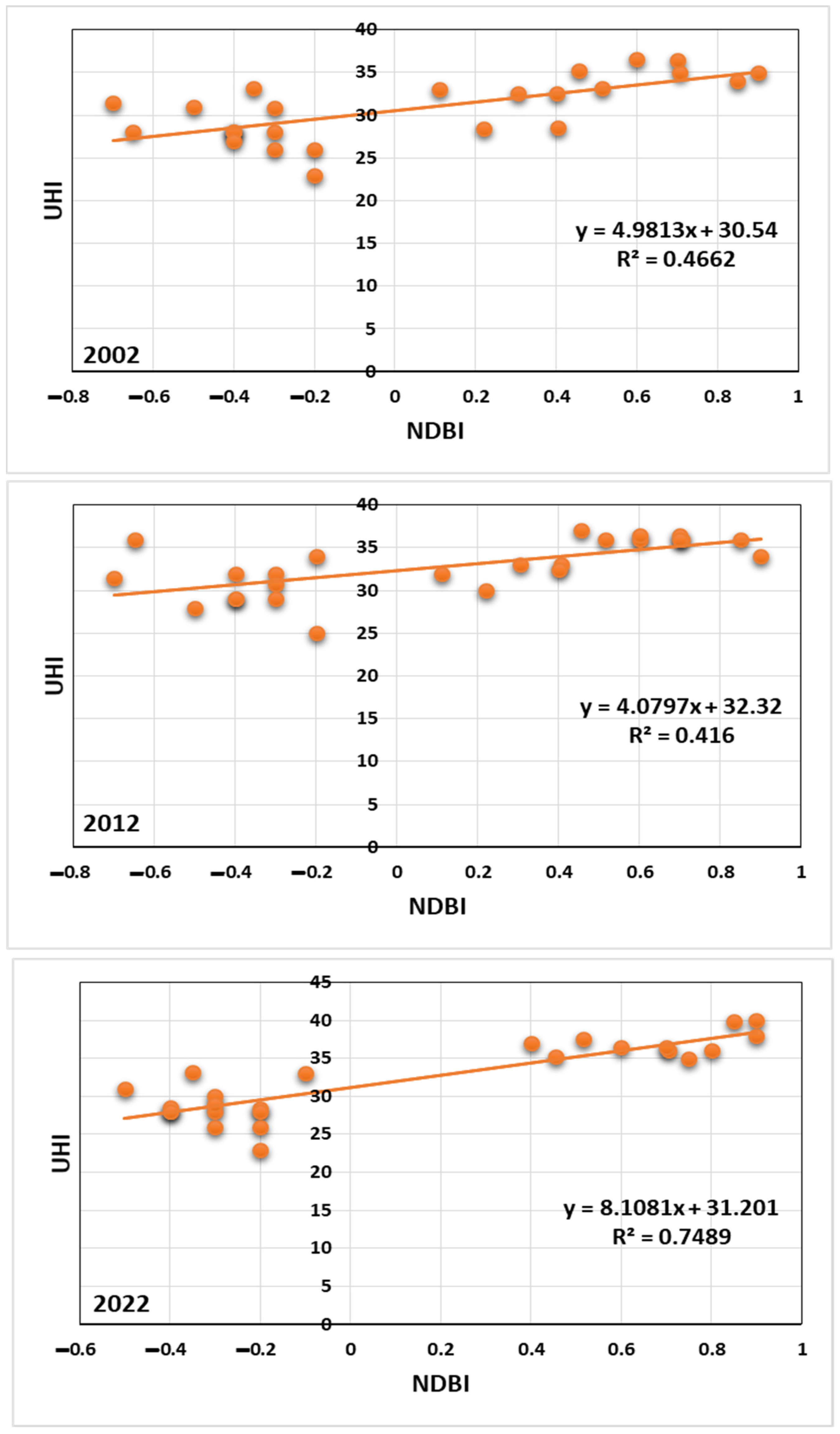
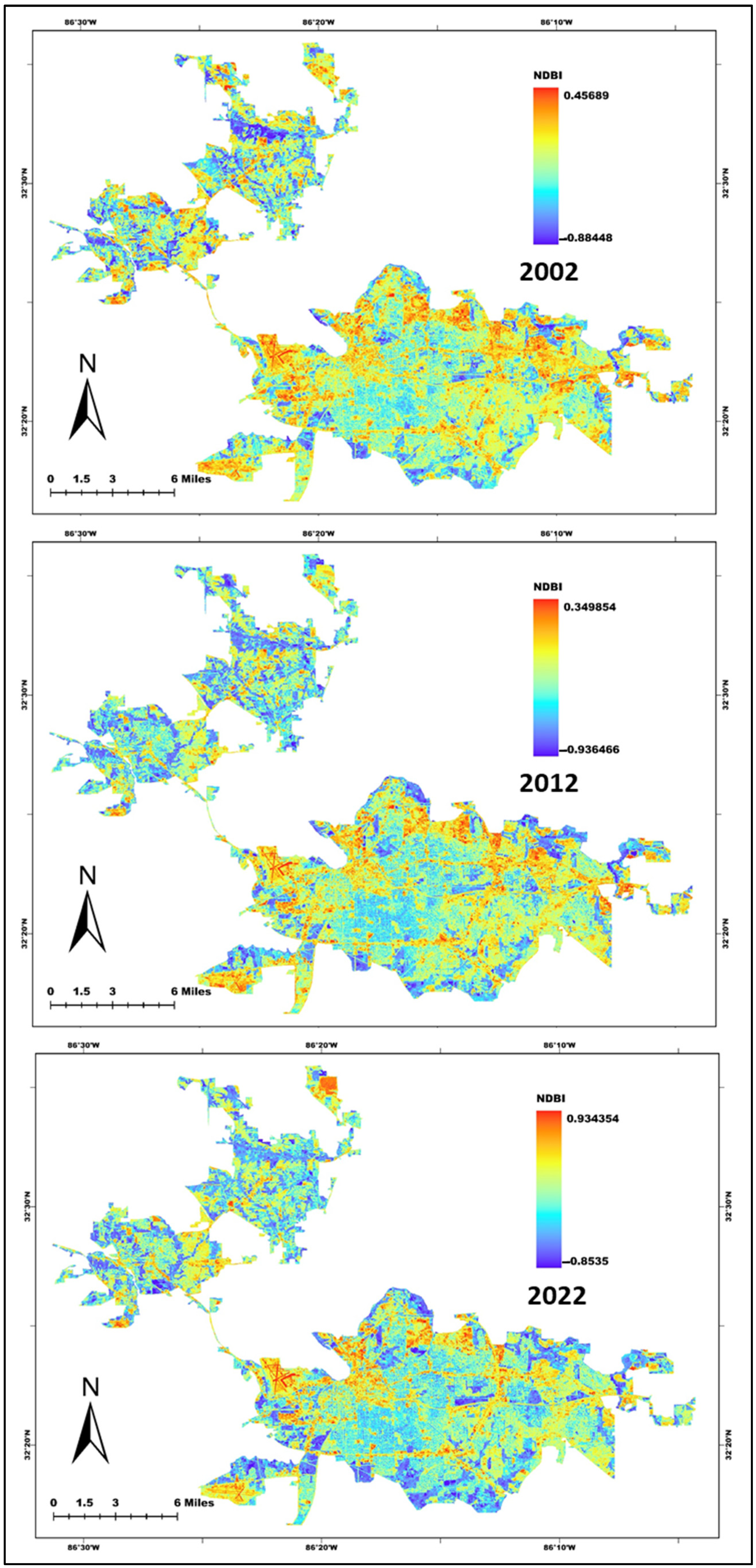
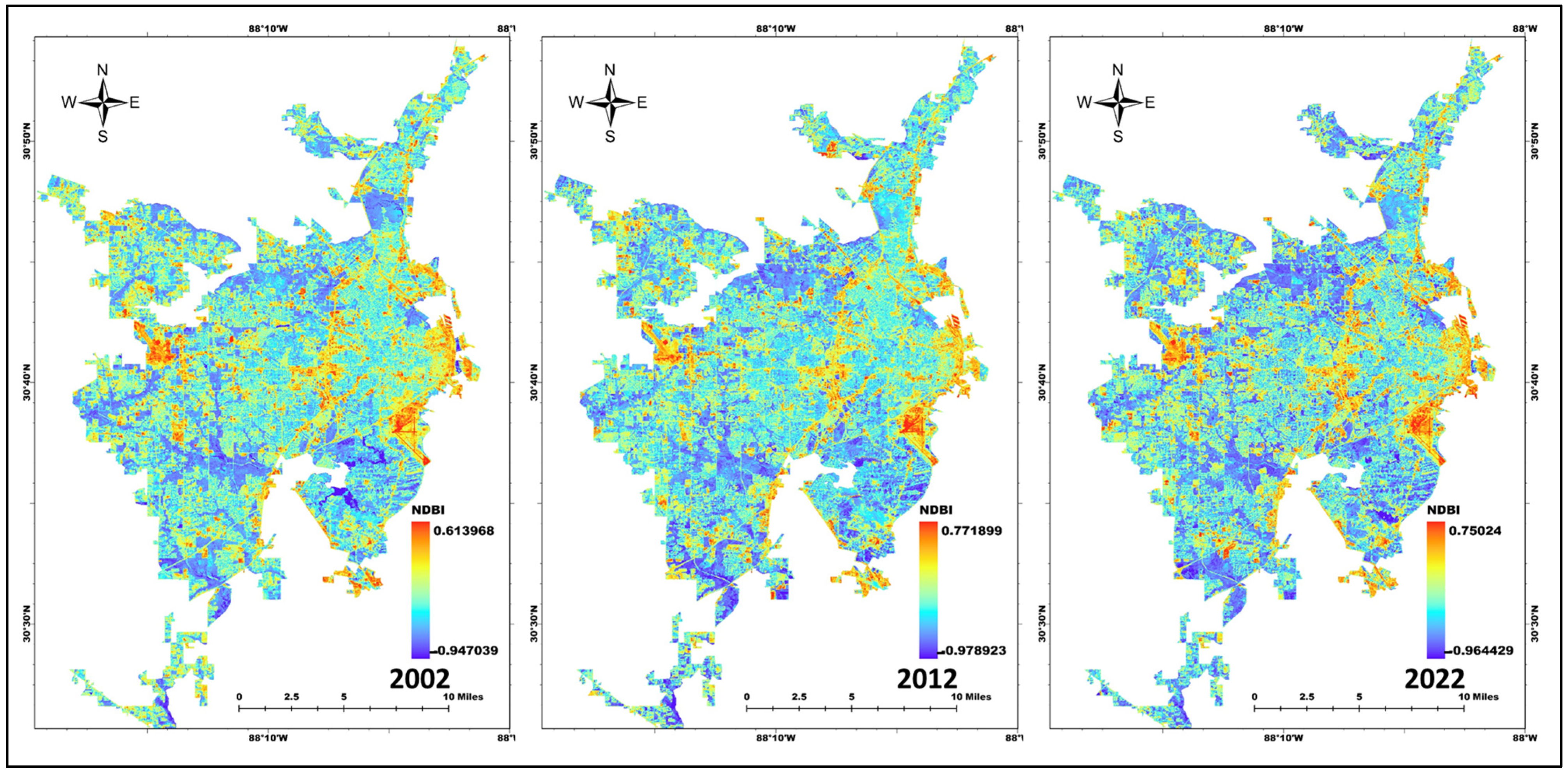
3.4. Spatiotemporal Variations of NDBI
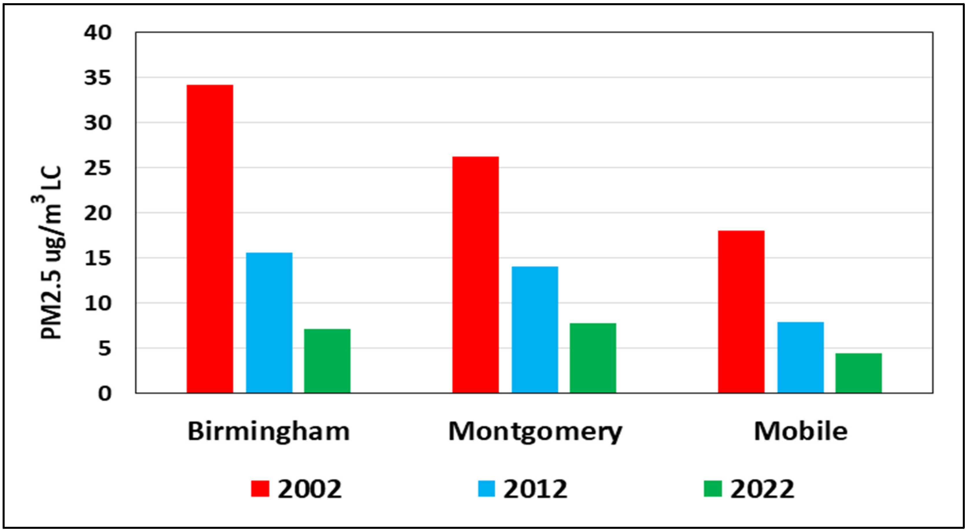
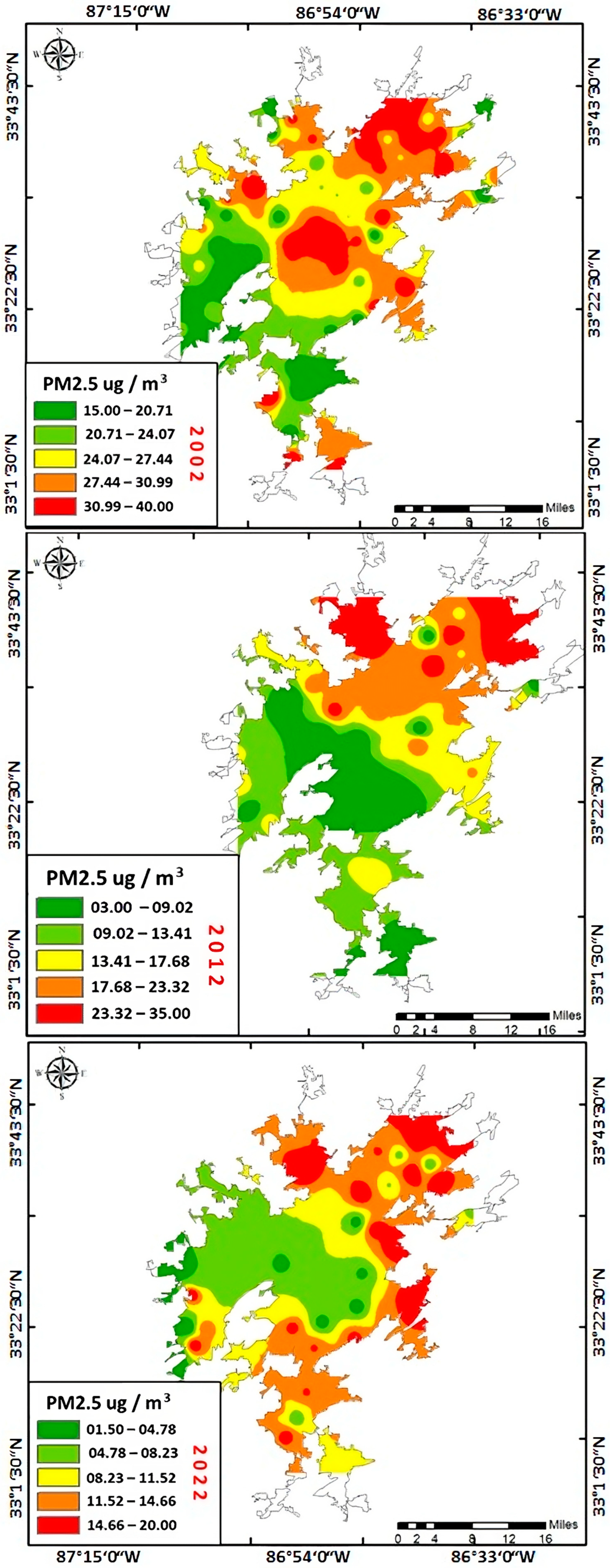
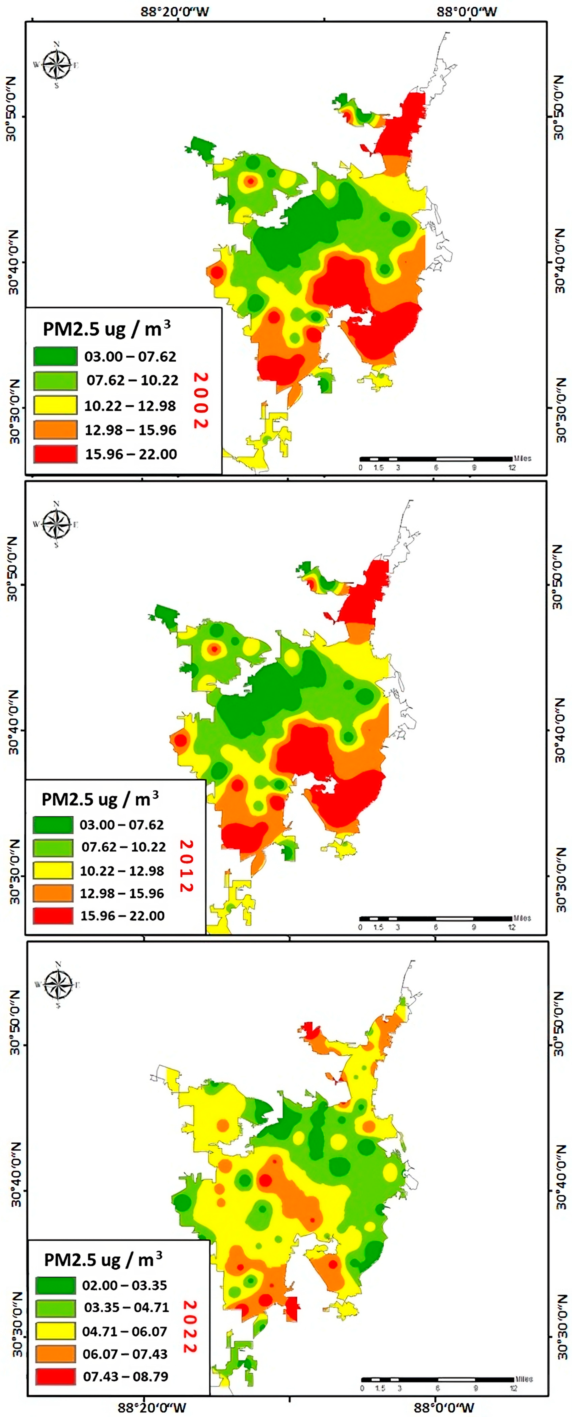
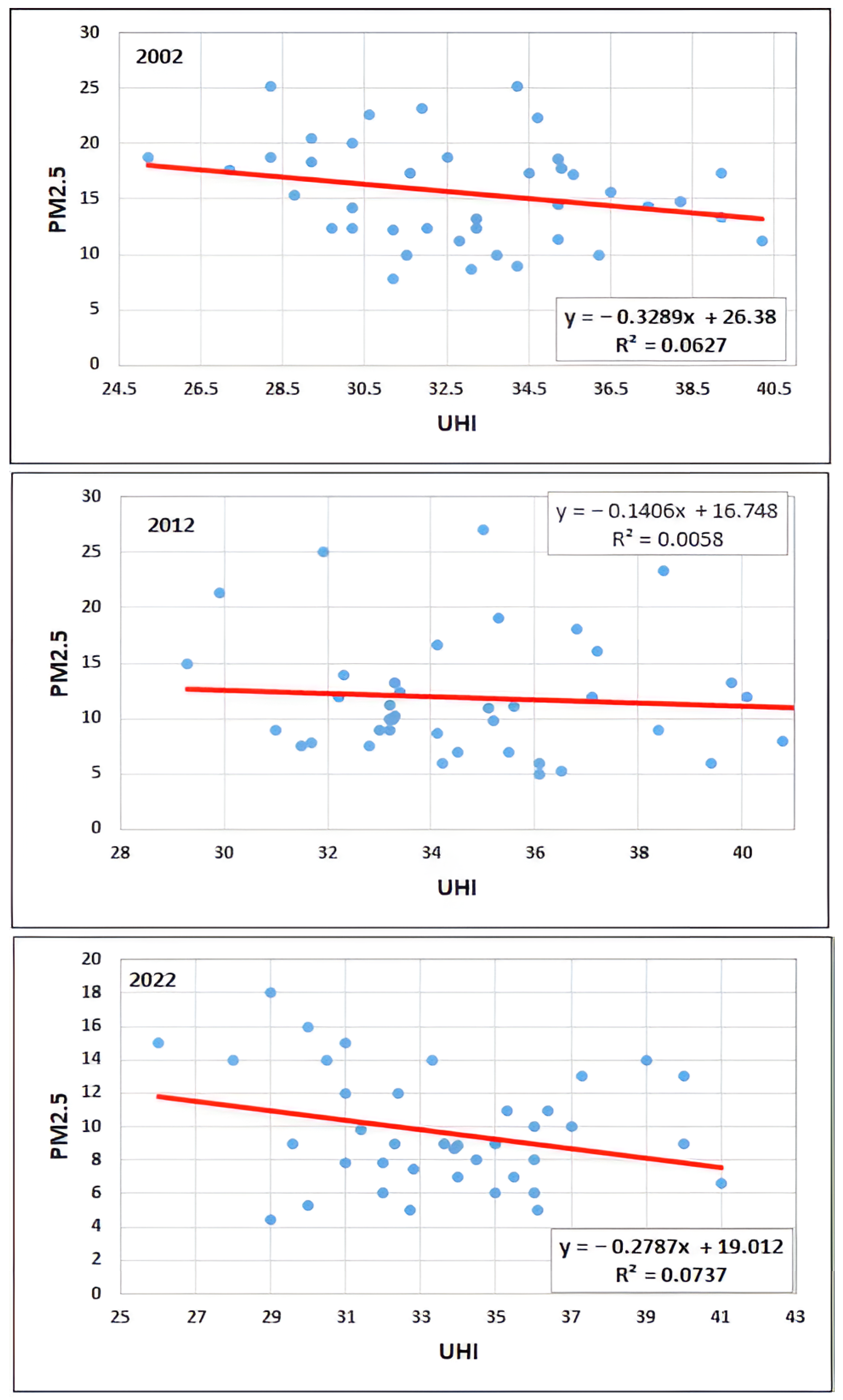
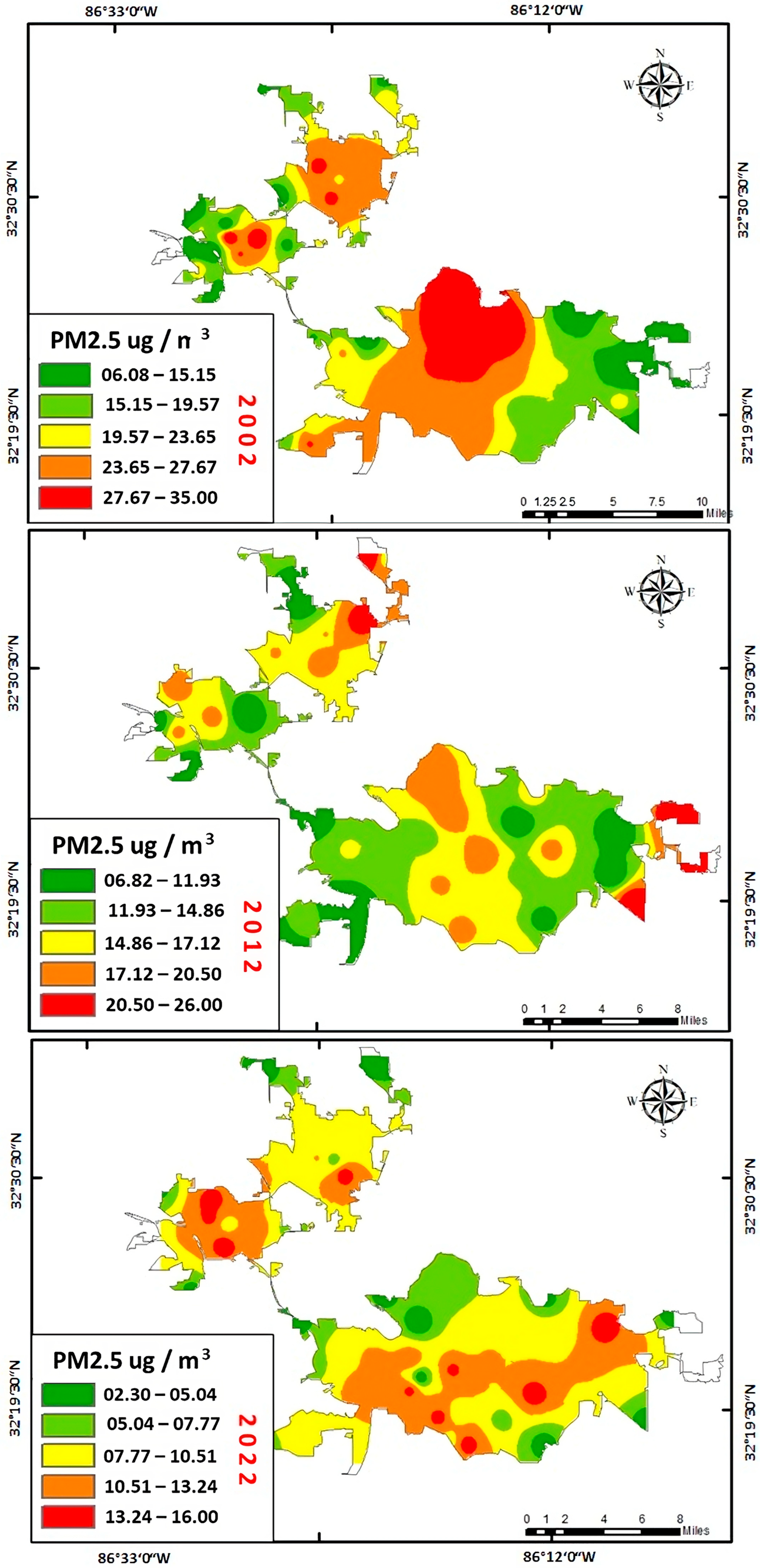
3.5. Spatiotemporal Variations of PM2.5 Concentration
3.6. PM2.5 Spatial Interpolation Model
4. Discussion
5. The Study Limitations
6. Conclusions
Author Contributions
Funding
Data Availability Statement
Conflicts of Interest
Appendix A
- TOA Radiance: Top of Atmosphere radiance
- MLQcal: DN value of pixel for radiance
- AL: The maximum radiance
- TOA Reflectance: Top of Atmosphere
- MLQcal: DN value of pixel for reflectance
- Aρ: The maximum reflectance
- Lλ: Spectral radiance
- Lmax: Maximum radiance
- Lmini: Minimum radiance
- Qcal: DN value of the pixel
- Qcalmax: DN value of pixel maximum
- Qcalmin: DN value of pixel minimum
- Oi: Correction value for bands 6 and 10
- K1 and K2 are the thermal constants of Radiance of bands 10 and 6 which can be identified in the metadata file associated with the satellite image.
- Lλ: Spectral radiance
- ԑv: Vegetation emissivity
- ԑs: Soil emissivity
- C: Surface roughness
- Ts: LST in Celsius (°C).
- BT: sensor BT (°C).
- λ: Average wavelength of bands 6 and 10.
- ԑλ Emissivity and ρ is (h x) which is equal to 1.438 × 10⁻² m/K.
- σ is the Boltzmann constant (1.38 × 10⁻²³ J/K).
- h is Planck’s constant (6.626 × 10⁻³⁴).
- c is the velocity of light (3 × 10⁸ m/s).
- UHI: Urban Heat Island.
- LST: Land Surface Temperature
- ∆Tu-r: UHI intensity
- Tu: Urban Temperature
- Tr: Rural Temperature
Appendix B

| Urban Area | Rural Area | Name of Station | Location of Station |
|---|---|---|---|
| Montgomery | Pike | Montgomery Airport AL, | 32.29 N–86.40 W |
| Birmingham | Shelby | Alabaster Shelby Co Air | 33.17 N–86.78 W |
| Mobile | Baldwin | Fairhope 3 NE, AL | 30.54 N–87.87 W |
| City | R2 Value | ||
|---|---|---|---|
| 2002 | 2012 | 2022 | |
| Birmingham | 0.89 | 0.93 | 0.95 |
| Montgomery | 0.85 | 0.89 | 0.92 |
| Mobile | 0.80 | 0.92 | 0.93 |
References
- Bettencourt, L.M.A. Urban Growth and the Emergent Statistics of Cities. Sci. Adv. 2020, 6, eaat8812. [Google Scholar] [CrossRef] [PubMed]
- Wang, J.; Yan, Z.-W. Urbanization-Related Warming in Local Temperature Records: A Review. Atmos. Ocean. Sci. Lett. 2016, 9, 129–138. [Google Scholar] [CrossRef]
- Ranagalage, M.; Ratnayake, S.S.; Dissanayake, D.; Kumar, L.; Wickremasinghe, H.; Vidanagama, J.; Cho, H.; Udagedara, S.; Jha, K.K.; Simwanda, M.; et al. Spatiotemporal Variation of Urban Heat Islands for Implementing Nature-Based Solutions: A Case Study of Kurunegala, Sri Lanka. ISPRS Int. J. Geo-Inf. 2020, 9, 461. [Google Scholar] [CrossRef]
- Dutta, D.; Rahman, A.; Paul, S.K.; Kundu, A. Impervious Surface Growth and Its Inter-Relationship with Vegetation Cover and Land Surface Temperature in Peri-Urban Areas of Delhi. Urban Clim. 2021, 37, 100799. [Google Scholar] [CrossRef]
- Buo, I.; Sagris, V.; Burdun, I.; Uuemaa, E. Estimating the Expansion of Urban Areas and Urban Heat Islands (UHI) in Ghana: A Case Study. Nat. Hazards 2021, 105, 1299–1321. [Google Scholar] [CrossRef]
- Shi, L.; Chu, E.; Anguelovski, I.; Aylett, A.; Debats, J.; Goh, K.; Schenk, T.; Seto, K.C.; Dodman, D.; Roberts, D.; et al. Roadmap towards Justice in Urban Climate Adaptation Research. Nat. Clim. Chang. 2016, 6, 131–137. [Google Scholar] [CrossRef]
- Du, P.; Chen, J.; Bai, X.; Han, W. Understanding the Seasonal Variations of Land Surface Temperature in Nanjing Urban Area Based on Local Climate Zone. Urban Clim. 2020, 33, 100657. [Google Scholar] [CrossRef]
- McDonnell, M.J.; MacGregor-Fors, I. The ecological future of cities. Science 2016, 352, 936–938. [Google Scholar] [CrossRef]
- Naim, N.H.; Kafy, A.-A. Assessment of Urban Thermal Field Variance Index and Defining the Relationship between Land Cover and Surface Temperature in Chattogram City: A Remote Sensing and Statistical Approach. Environ. Chall. 2021, 4, 100107. [Google Scholar] [CrossRef]
- Liu, P.; Jia, S.; Han, R.; Liu, Y.; Lu, X.; Zhang, H. RS and GIS Supported Urban LULC and UHI Change Simulation and Assessment. J. Sens. 2020, 2020, 5863164. [Google Scholar] [CrossRef]
- Martilli, A.; Krayenhoff, E.S.; Nazarian, N. Is the Urban Heat Island Intensity Relevant for Heat Mitigation Studies? Urban Clim. 2020, 31, 100541. [Google Scholar] [CrossRef]
- Qiao, Z.; Lu, Y.; He, T.; Wu, F.; Xu, X.; Liu, L.; Wang, F.; Sun, Z.; Han, D. Spatial Expansion Paths of Urban Heat Islands in Chinese Cities: Analysis from a Dynamic Topological Perspective for the Improvement of Climate Resilience. Resour. Conserv. Recycl. 2023, 188, 106680. [Google Scholar] [CrossRef]
- Atasoy, M. Assessing the Impacts of Land-Use/Land-Cover Change on the Development of Urban Heat Island Effects. Environ. Dev. Sustain. 2020, 22, 7547–7557. [Google Scholar] [CrossRef]
- Shahfahad; Rihan, M.; Naikoo, M.W.; Ali, M.A.; Usmani, T.M.; Rahman, A. Urban Heat Island Dynamics in Response to Land-Use/Land-Cover Change in the Coastal City of Mumbai. J. Indian Soc. Remote Sens. 2021, 49, 2227–2247. [Google Scholar] [CrossRef]
- Shahfahad; Talukdar, S.; Rihan, M.; Hang, H.T.; Bhaskaran, S.; Rahman, A. Modelling Urban Heat Island (UHI) and Thermal Field Variation and Their Relationship with Land Use Indices over Delhi and Mumbai Metro Cities. Environ. Dev. Sustain. 2022, 24, 3762–3790. [Google Scholar] [CrossRef]
- Stowell, J.D.; Bi, J.; Al-Hamdan, M.Z.; Lee, H.J.; Lee, S.-M.; Freedman, F.; Kinney, P.L.; Liu, Y. Estimating PM 2.5 in Southern California Using Satellite Data: Factors That Affect Model Performance. Environ. Res. Lett. 2020, 15, 094004. [Google Scholar] [CrossRef]
- Wang, Y.; Du, H.; Xu, Y.; Lu, D.; Wang, X.; Guo, Z. Temporal and Spatial Variation Relationship and Influence Factors on Surface Urban Heat Island and Ozone Pollution in the Yangtze River Delta, China. Sci. Total Environ. 2018, 631–632, 921–933. [Google Scholar] [CrossRef]
- Li, H.; Meier, F.; Lee, X.; Chakraborty, T.; Liu, J.; Schaap, M.; Sodoudi, S. Interaction between Urban Heat Island and Urban Pollution Island during Summer in Berlin. Sci. Total Environ. 2018, 636, 818–828. [Google Scholar] [CrossRef]
- Guo, G.; Zhou, X.; Wu, Z.; Xiao, R.; Chen, Y. Characterizing the Impact of Urban Morphology Heterogeneity on Land Surface Temperature in Guangzhou, China. Environ. Model. Softw. 2016, 84, 427–439. [Google Scholar] [CrossRef]
- Yang, G.; Ren, G.; Zhang, P.; Xue, X.; Tysa, S.K.; Jia, W.; Qin, Y.; Zheng, X.; Zhang, S. PM 2.5 Influence on Urban Heat Island (UHI) Effect in Beijing and the Possible Mechanisms. Geophys. Res. Atmos. 2021, 126, e2021JD035227. [Google Scholar] [CrossRef]
- Von Bismarck-Osten, C.; Birmili, W.; Ketzel, M.; Massling, A.; Petäjä, T.; Weber, S. Characterization of Parameters Influencing the Spatio-Temporal Variability of Urban Particle Number Size Distributions in Four European Cities. Atmos. Environ. 2013, 77, 415–429. [Google Scholar] [CrossRef]
- Borge, R.; Narros, A.; Artíñano, B.; Yagüe, C.; Gómez-Moreno, F.J.; De La Paz, D.; Román-Cascón, C.; Díaz, E.; Maqueda, G.; Sastre, M.; et al. Assessment of Microscale Spatio-Temporal Variation of Air Pollution at an Urban Hotspot in Madrid (Spain) through an Extensive Field Campaign. Atmos. Environ. 2016, 140, 432–445. [Google Scholar] [CrossRef]
- Zhao, L.; Oppenheimer, M.; Zhu, Q.; Baldwin, J.W.; Ebi, K.L.; Bou-Zeid, E.; Guan, K.; Liu, X. Interactions between Urban Heat Islands and Heat Waves. Environ. Res. Lett. 2018, 13, 034003. [Google Scholar] [CrossRef]
- Yue, W.; Liu, X.; Zhou, Y.; Liu, Y. Impacts of Urban Configuration on Urban Heat Island: An Empirical Study in China Mega-Cities. Sci. Total Environ. 2019, 671, 1036–1046. [Google Scholar] [CrossRef]
- Zhou, D.; Zhao, S.; Zhang, L.; Sun, G.; Liu, Y. The Footprint of Urban Heat Island Effect in China. Sci. Rep. 2015, 5, 11160. [Google Scholar] [CrossRef] [PubMed]
- Giridharan, R.; Emmanuel, R. The Impact of Urban Compactness, Comfort Strategies and Energy Consumption on Tropical Urban Heat Island Intensity: A Review. Sustain. Cities Soc. 2018, 40, 677–687. [Google Scholar] [CrossRef]
- Zhou, B.; Rybski, D.; Kropp, J.P. The Role of City Size and Urban Form in the Surface Urban Heat Island. Sci. Rep. 2017, 7, 4791. [Google Scholar] [CrossRef]
- Kang, H.; Zhu, B.; De Leeuw, G.; Yu, B.; Van Der A, R.J.; Lu, W. Impact of Urban Heat Island on Inorganic Aerosol in the Lower Free Troposphere: A Case Study in Hangzhou, China. Atmos. Chem. Phys. 2022, 22, 10623–10634. [Google Scholar] [CrossRef]
- Hinkel, K.M.; Nelson, F.E.; Klene, A.E.; Bell, J.H. The Urban Heat Island in Winter at Barrow, Alaska. Int. J. Climatol. 2003, 23, 1889–1905. [Google Scholar] [CrossRef]
- Ackley, J.W.; Angilletta, M.J.; DeNardo, D.; Sullivan, B.; Wu, J. Urban Heat Island Mitigation Strategies and Lizard Thermal Ecology: Landscaping Can Quadruple Potential Activity Time in an Arid City. Urban Ecosyst. 2015, 18, 1447–1459. [Google Scholar] [CrossRef]
- Tan, J.; Zheng, Y.; Tang, X.; Guo, C.; Li, L.; Song, G.; Zhen, X.; Yuan, D.; Kalkstein, A.J.; Li, F.; et al. The Urban Heat Island and Its Impact on Heat Waves and Human Health in Shanghai. Int. J. Biometeorol. 2010, 54, 75–84. [Google Scholar] [CrossRef] [PubMed]
- Simwanda, M.; Ranagalage, M.; Estoque, R.C.; Murayama, Y. Spatial Analysis of Surface Urban Heat Islands in Four Rapidly Growing African Cities. Remote Sens. 2019, 11, 1645. [Google Scholar] [CrossRef]
- Dian, C.; Pongrácz, R.; Dezső, Z.; Bartholy, J. Annual and Monthly Analysis of Surface Urban Heat Island Intensity with Respect to the Local Climate Zones in Budapest. Urban Clim. 2020, 31, 100573. [Google Scholar] [CrossRef]
- Dissanayake, D.M.S.L.B.; Morimoto, T.; Ranagalage, M.; Murayama, Y. Land-Use/Land-Cover Changes and Their Impact on Surface Urban Heat Islands: Case Study of Kandy City, Sri Lanka. Climate 2019, 7, 99. [Google Scholar] [CrossRef]
- Balew, A.; Semaw, F. Impacts of Land-Use and Land-Cover Changes on Surface Urban Heat Islands in Addis Ababa City and Its Surrounding. Environ. Dev. Sustain. 2022, 24, 832–866. [Google Scholar] [CrossRef]
- Cheval, S.; Popa, A.-M.; Șandric, I.; Iojă, I.-C. Exploratory Analysis of Cooling Effect of Urban Lakes on Land Surface Temperature in Bucharest (Romania) Using Landsat Imagery. Urban Clim. 2020, 34, 100696. [Google Scholar] [CrossRef]
- Rousta, I.; Sarif, M.; Gupta, R.; Olafsson, H.; Ranagalage, M.; Murayama, Y.; Zhang, H.; Mushore, T. Spatiotemporal Analysis of Land Use/Land Cover and Its Effects on Surface Urban Heat Island Using Landsat Data: A Case Study of Metropolitan City Tehran (1988–2018). Sustainability 2018, 10, 4433. [Google Scholar] [CrossRef]
- Han, D.; Zhang, T.; Qin, Y.; Tan, Y.; Liu, J. A Comparative Review on the Mitigation Strategies of Urban Heat Island (UHI): A Pathway for Sustainable Urban Development. Clim. Dev. 2023, 15, 379–403. [Google Scholar] [CrossRef]
- Shen, P.; Wang, M.; Liu, J.; Ji, Y. Hourly Air Temperature Projection in Future Urban Area by Coupling Climate Change and Urban Heat Island Effect. Energy Build. 2023, 279, 112676. [Google Scholar] [CrossRef]
- Gedzelman, S.D.; Austin, S.; Cermak, R.; Stefano, N.; Partridge, S.; Quesenberry, S.; Robinson, D.A. Mesoscale Aspects of the Urban Heat Island around New York City. Theor. Appl. Climatol. 2003, 75, 29–42. [Google Scholar] [CrossRef]
- Lokoshchenko, M.A.; Alekseeva, L.I. Influence of Meteorological Parameters on the Urban Heat Island in Moscow. Atmosphere 2023, 14, 507. [Google Scholar] [CrossRef]
- Sofer, M.; Potchter, O. The Urban Heat Island of a City in an Arid Zone: The Case of Eilat, Israel. Theor. Appl. Climatol. 2006, 85, 81–88. [Google Scholar] [CrossRef]
- Murata, A.; Sasaki, H.; Hanafusa, M.; Kurihara, K. Estimation of Urban Heat Island Intensity Using Biases in Surface Air Temperature Simulated by a Nonhydrostatic Regional Climate Model. Theor. Appl. Clim. 2013, 112, 351–361. [Google Scholar] [CrossRef]
- Gao, Y.; Zhao, J.; Han, L. Exploring the Spatial Heterogeneity of Urban Heat Island Effect and Its Relationship to Block Morphology with the Geographically Weighted Regression Model. Sustain. Cities Soc. 2022, 76, 103431. [Google Scholar] [CrossRef]
- Hu, D.; Meng, Q.; Schlink, U.; Hertel, D.; Liu, W.; Zhao, M.; Guo, F. How Do Urban Morphological Blocks Shape Spatial Patterns of Land Surface Temperature over Different Seasons? A Multifactorial Driving Analysis of Beijing, China. Int. J. Appl. Earth Obs. Geoinf. 2022, 106, 102648. [Google Scholar] [CrossRef]
- Ivajnšič, D.; Kaligarič, M.; Žiberna, I. Geographically Weighted Regression of the Urban Heat Island of a Small City. Appl. Geogr. 2014, 53, 341–353. [Google Scholar] [CrossRef]
- Zhang, L.; Shi, X.; Chang, Q. Exploring Adaptive UHI Mitigation Solutions by Spatial Heterogeneity of Land Surface Temperature and Its Relationship to Urban Morphology in Historical Downtown Blocks, Beijing. Land 2022, 11, 544. [Google Scholar] [CrossRef]
- Xiang, Y.; Huang, C.; Huang, X.; Zhou, Z.; Wang, X. Seasonal Variations of the Dominant Factors for Spatial Heterogeneity and Time Inconsistency of Land Surface Temperature in an Urban Agglomeration of Central China. Sustain. Cities Soc. 2021, 75, 103285. [Google Scholar] [CrossRef]
- Taha, H. Meso-Urban Meteorological and Photochemical Modeling of Heat Island Mitigation. Atmos. Environ. 2008, 42, 8795–8809. [Google Scholar] [CrossRef]
- Weng, Q.; Fu, P. Modeling Diurnal Land Temperature Cycles over Los Angeles Using Downscaled GOES Imagery. ISPRS J. Photogramm. Remote Sens. 2014, 97, 78–88. [Google Scholar] [CrossRef]
- Vahmani, P.; Ban-Weiss, G.A. Impact of Remotely Sensed Albedo and Vegetation Fraction on Simulation of Urban Climate in WRF-Urban Canopy Model: A Case Study of the Urban Heat Island in Los Angeles: Satellite-Supported Urban Climate Model. J. Geophys. Res. Atmos. 2016, 121, 1511–1531. [Google Scholar] [CrossRef]
- Bornstein, R.; Lin, Q. Urban Heat Islands and Summertime Convective Thunderstorms in Atlanta: Three Case Studies. Atmos. Environ. 2000, 34, 507–516. [Google Scholar] [CrossRef]
- Chun, B.; Guhathakurta, S. Daytime and Nighttime Urban Heat Islands Statistical Models for Atlanta. Environ. Plan. B Urban Anal. City Sci. 2017, 44, 308–327. [Google Scholar] [CrossRef]
- Lo, C.P.; Quattrochi, D.A. Land-Use and Land-Cover Change, Urban Heat Island Phenomenon, and Health Implications: A Remote Sensing Approach. Photogramm. Eng. Remote Sens. 2003, 69, 1053–1063. [Google Scholar] [CrossRef]
- Liao, D.; Zhu, H.; Jiang, P. Study of Urban Heat Island Index Methods for Urban Agglomerations (Hilly Terrain) in Chongqing. Theor. Appl. Clim. 2021, 143, 279–289. [Google Scholar] [CrossRef]
- Ying, Q.; Wu, L.; Zhang, H. Local and Inter-Regional Contributions to PM2.5 Nitrate and Sulfate in China. Atmos. Environ. 2014, 94, 582–592. [Google Scholar] [CrossRef]
- Zhang, H.; Hu, J.; Kleeman, M.; Ying, Q. Source Apportionment of Sulfate and Nitrate Particulate Matter in the Eastern United States and Effectiveness of Emission Control Programs. Sci. Total Environ. 2014, 490, 171–181. [Google Scholar] [CrossRef]
- Kim, Y.-H.; Baik, J.-J. Daily Maximum Urban Heat Island Intensity in Large Cities of Korea. Theor. Appl. Clim. 2004, 79, 151–164. [Google Scholar] [CrossRef]
- Khorrami, B.; Gunduz, O. Spatio-Temporal Interactions of Surface Urban Heat Island and Its Spectral Indicators: A Case Study from Istanbul Metropolitan Area, Turkey. Environ. Monit. Assess. 2020, 192, 386. [Google Scholar] [CrossRef]
- Peng, S.; Feng, Z.; Liao, H.; Huang, B.; Peng, S.; Zhou, T. Spatial-Temporal Pattern of, and Driving Forces for, Urban Heat Island in China. Ecol. Indic. 2019, 96, 127–132. [Google Scholar] [CrossRef]
- Xiang, Y.; Cen, Q.; Peng, C.; Huang, C.; Wu, C.; Teng, M.; Zhou, Z. Surface Urban Heat Island Mitigation Network Construction Utilizing Source-Sink Theory and Local Climate Zones. Build. Environ. 2023, 243, 110717. [Google Scholar] [CrossRef]
- Geng, X.; Zhang, D.; Li, C.; Yuan, Y.; Yu, Z.; Wang, X. Impacts of Climatic Zones on Urban Heat Island: Spatiotemporal Variations, Trends, and Drivers in China from 2001–2020. Sustain. Cities Soc. 2023, 89, 104303. [Google Scholar] [CrossRef]
- Li, Y.; Sun, Y.; Li, J.; Gao, C. Socioeconomic Drivers of Urban Heat Island Effect: Empirical Evidence from Major Chinese Cities. Sustain. Cities Soc. 2020, 63, 102425. [Google Scholar] [CrossRef]
- Meng, F.; Ren, G.; Zhang, R. Impacts of UHI on Heating and Cooling Loads in Residential Buildings in Cities of Different Sizes in Beijing–Tianjin–Hebei Region in China. Atmosphere 2023, 14, 1193. [Google Scholar] [CrossRef]
- Sabrin, S.; Karimi, M.; Nazari, R. Modeling Heat Island Exposure and Vulnerability Utilizing Earth Observations and Social Drivers: A Case Study for Alabama, USA. Build. Environ. 2022, 226, 109686. [Google Scholar] [CrossRef]
- Abbas, W.; Ismael, H. Assessment of Constructing Canopy Urban Heat Island Temperatures from Thermal Images: An Integrated Multi-Scale Approach. Sci. Afr. 2020, 10, e00607. [Google Scholar] [CrossRef]
- Wang, Z.; Shafieezadeh, A. ESC: An Efficient Error-Based Stopping Criterion for Kriging-Based Reliability Analysis Methods. Struct. Multidiscip. Optim. 2019, 59, 1621–1637. [Google Scholar] [CrossRef]
- Xu, C.; Wang, J.; Hu, M.; Wang, W. A New Method for Interpolation of Missing Air Quality Data at Monitor Stations. Environ. Int. 2022, 169, 107538. [Google Scholar] [CrossRef]
- Wei, P.; Xie, S.; Huang, L.; Liu, L.; Tang, Y.; Zhang, Y.; Wu, H.; Xue, Z.; Ren, D. Spatial Interpolation of PM2.5 Concentrations during Holidays in South-Central China Considering Multiple Factors. Atmos. Pollut. Res. 2022, 13, 101480. [Google Scholar] [CrossRef]
- Yang, J.; Zhao, Y.; Zou, Y.; Xia, D.; Lou, S.; Liu, W.; Ji, K. Effects of Tree Species and Layout on the Outdoor Thermal Environment of Squares in Hot-Humid Areas of China. Buildings 2022, 12, 1867. [Google Scholar] [CrossRef]
- Tang, Y.; Xie, S.; Huang, L.; Liu, L.; Wei, P.; Zhang, Y.; Meng, C. Spatial Estimation of Regional PM2.5 Concentrations with GWR Models Using PCA and RBF Interpolation Optimization. Remote Sens. 2022, 14, 5626. [Google Scholar] [CrossRef]
- Ghosh, S.; Kumar, D.; Kumari, R. Assessing Spatiotemporal Dynamics of Land Surface Temperature and Satellite-Derived Indices for New Town Development and Suburbanization Planning. Urban Gov. 2022, 2, 144–156. [Google Scholar] [CrossRef]
- Kim, K.; Jeon, J.; Jung, H.; Kim, T.K.; Hong, J.; Jeon, G.-S.; Kim, H.S. PM2.5 Reduction Capacities and Their Relation to Morphological and Physiological Traits in 13 Landscaping Tree Species. Urban For. Urban Green. 2022, 70, 127526. [Google Scholar] [CrossRef]
- Wu, H.; Wang, T.; Wang, Q.; Cao, Y.; Qu, Y.; Nie, D. Radiative Effects and Chemical Compositions of Fine Particles Modulating Urban Heat Island in Nanjing, China. Atmos. Environ. 2021, 247, 118201. [Google Scholar] [CrossRef]
- Sheridan, S.C. A Survey of Public Perception and Response to Heat Warnings across Four North American Cities: An Evaluation of Municipal Effectiveness. Int. J. Biometeorol. 2007, 52, 3–15. [Google Scholar] [CrossRef]
- Masson, V. Urban Surface Modeling and the Meso-Scale Impact of Cities. Theor. Appl. Climatol. 2006, 84, 35–45. [Google Scholar] [CrossRef]
- Pal, S.; Xueref-Remy, I.; Ammoura, L.; Chazette, P.; Gibert, F.; Royer, P.; Dieudonné, E.; Dupont, J.-C.; Haeffelin, M.; Lac, C.; et al. Spatio-Temporal Variability of the Atmospheric Boundary Layer Depth over the Paris Agglomeration: An Assessment of the Impact of the Urban Heat Island Intensity. Atmos. Environ. 2012, 63, 261–275. [Google Scholar] [CrossRef]
- Fallmann, J.; Forkel, R.; Emeis, S. Secondary Effects of Urban Heat Island Mitigation Measures on Air Quality. Atmos. Environ. 2016, 125, 199–211. [Google Scholar] [CrossRef]
- Balew, A.; Korme, T. Monitoring Land Surface Temperature in Bahir Dar City and Its Surrounding Using Landsat Images. Egypt. J. Remote Sens. Space Sci. 2020, 23, 371–386. [Google Scholar] [CrossRef]
- Shirangi, A.; Nieuwenhuijsen, M.; Vienneau, D.; Holman, C.D.J. Living near Agricultural Pesticide Applications and the Risk of Adverse Reproductive Outcomes: A Review of the Literature. Paediatr. Perinat. Epidemiol. 2011, 25, 172–191. [Google Scholar] [CrossRef]
- Guha, S.; Govil, H.; Gill, N.; Dey, A. Analytical Study on the Relationship between Land Surface Temperature and Land Use/Land Cover Indices. Ann. GIS 2020, 26, 201–216. [Google Scholar] [CrossRef]
- Zekar, A.; Milojevic-Dupont, N.; Zumwald, M.; Wagner, F.; Creutzig, F. Urban Form Features Determine Spatio-Temporal Variation of Ambient Temperature: A Comparative Study of Three European Cities. Urban Clim. 2023, 49, 101467. [Google Scholar] [CrossRef]
- Kumari, P.; Garg, V.; Kumar, R.; Kumar, K. Impact of Urban Heat Island Formation on Energy Consumption in Delhi. Urban Clim. 2021, 36, 100763. [Google Scholar] [CrossRef]
- Sharma, A.; Kumar, V.; Shahzad, B.; Tanveer, M.; Sidhu, G.P.S.; Handa, N.; Kohli, S.K.; Yadav, P.; Bali, A.S.; Parihar, R.D.; et al. Worldwide Pesticide Usage and Its Impacts on Ecosystem. SN Appl. Sci. 2019, 1, 1446. [Google Scholar] [CrossRef]
- Sobrino, J.A.; Oltra-Carrió, R.; Sòria, G.; Bianchi, R.; Paganini, M. Impact of Spatial Resolution and Satellite Overpass Time on Evaluation of the Surface Urban Heat Island Effects. Remote Sens. Environ. 2012, 117, 50–56. [Google Scholar] [CrossRef]
- Liu, Z.; Lai, J.; Zhan, W.; Bechtel, B.; Voogt, J.; Quan, J.; Hu, L.; Fu, P.; Huang, F.; Li, L.; et al. Urban Heat Islands Significantly Reduced by COVID-19 Lockdown. Geophys. Res. Lett. 2022, 49, e2021GL096842. [Google Scholar] [CrossRef]
- San Martini, F.M.; Hasenkopf, C.A.; Roberts, D.C. Statistical Analysis of PM2.5 Observations from Diplomatic Facilities in China. Atmos. Environ. 2015, 110, 174–185. [Google Scholar] [CrossRef]
- Sharma, R.; Pradhan, L.; Kumari, M.; Bhattacharya, P. Assessing Urban Heat Islands and Thermal Comfort in Noida City Using Geospatial Technology. Urban Clim. 2021, 35, 100751. [Google Scholar] [CrossRef]
- Hong, J.; Lee, M.; Huh, W.; Kim, T.K.; Jeon, J.; Lee, H.; Kim, K.; Byeon, S.; Park, C.; Kim, H.S. Comparisons of PM2.5 Mitigation with Stand Characteristics between Evergreen Korean Pine Plantations and Deciduous Broad-Leaved Forests in the Republic of Korea. Environ. Pollut. 2023, 334, 122240. [Google Scholar] [CrossRef]
- Lee, H.; Jeon, J.; Lee, M.; Kim, H.S. Seasonal Contrasting Effects of PM2.5 on Forest Productivity in Peri-urban Region of Seoul Metropolitan Area, Republic of Korea. Agric. For. Meteorol. 2022, 325, 109149. [Google Scholar] [CrossRef]
- Chen, Y.; Ke, X.; Min, M.; Zhang, Y.; Dai, Y.; Tang, L. Do We Need More Urban Green Space to Alleviate PM2.5 Pollution? A Case Study in Wuhan, China. Land 2022, 11, 776. [Google Scholar] [CrossRef]
- Yin, S.; Zhang, X.; Yu, A.; Sun, N.; Lyu, J.; Zhu, P.; Liu, C. Determining PM2.5 Dry Deposition Velocity on Plant Leaves: An Indirect Experimental Method. Urban For. Urban Green. 2019, 46, 126467. [Google Scholar] [CrossRef]


| Sensor | Path/Raw | Location | Acquisition Date | Time (GMT) | K1 | K2 | Resolution (PAN/MS/TIRS) |
|---|---|---|---|---|---|---|---|
| Landsat 7 ETM+ | 020/037 | 32.29 N–86.40 W | 7 July 2002 | 18:26:00 | 607.56 | 1260.56 | 15/30/60 m |
| 021/038 | 33.17 N–86.78 W | ||||||
| 021/039 | 30.54 N–87.87 W | ||||||
| Landsat 8 OLI/TIRS | 020/037 | 32.29 N–86.40 W | 7 August 2012 | 18:45:03 | 774.88 | 1321.07 | 15/30/100 m |
| 021/038 | 33.17 N–86.78 W | ||||||
| 021/039 | 30.54 N–87.87 W | ||||||
| Landsat 8 OLI/TIRS | 020/037 | 32.29 N–86.40 W | 7 July 2022 | 18:59:17 | 774.88 | 1321.07 | 15/30/100 m |
| 021/038 | 33.17 N–86.78 W | ||||||
| 021/039 | 30.54 N–87.87 W |
| Year | User’s Accuracy (%) | Producer’s Accuracy (%) | Overall Accuracy (%) | Kappa Coefficient (%) |
|---|---|---|---|---|
| 2002 | 96.6 | 92.3 | 92.3 | 0.93 |
| 2012 | 95.4 | 89.4 | 93.5 | 0.95 |
| 2022 | 94.8 | 88.0 | 92.80 | 0.90 |
| Birmingham LULC Class | 2002 | 2012 | 2022 | |||
|---|---|---|---|---|---|---|
| Area in sq. km | Area in % | Area in sq. km | Area in % | Area in sq. km | Area in % | |
| Built-up area | 217.60 | 13.10 | 242.00 | 14.56 | 294.50 | 17.73 |
| Cropland | 478.60 | 28.80 | 367.25 | 22.10 | 465.81 | 28.03 |
| Forest | 957.18 | 57.61 | 1042.63 | 62.75 | 891.88 | 53.70 |
| Water bodies | 8.05 | 0.48 | 9.53 | 0.57 | 9.22 | 0.55 |
| Total | 1,661,410 | 100 | 1,661,410 | 100 | 1,661,410 | 100 |
| Montgomery LULC Class | 2002 | 2012 | 2022 | |||
| Area in sq. km | Area in % | Area in sq. km | Area in % | Area in sq. km | Area in % | |
| Built-up area | 170.48 | 42.60 | 182.20 | 45.53 | 205.57 | 51.37 |
| Cropland | 47.54 | 11.88 | 59.48 | 14.86 | 55.40 | 13.84 |
| Forest | 179.84 | 44.94 | 156.35 | 39.07 | 136.07 | 34.00 |
| Water bodies | 2.3292 | 0.58 | 2.169 | 0.54 | 3.164 | 0.79 |
| Total | 4,001,994 | 100 | 4,001,994 | 100 | 4,001,994 | 100 |
| Mobile LULC Class | 2002 | 2012 | 2022 | |||
| Area in sq. km | Area in % | Area in sq. km | Area in % | Area in sq. km | Area in % | |
| Built-up area | 184.06 | 26.91 | 211.22 | 30.88 | 285.13 | 41.68 |
| Cropland | 130.26 | 19.04 | 120.78 | 17.66 | 90.97 | 13.30 |
| Forest | 359.20 | 52.51 | 342.21 | 50.02 | 295.47 | 43.19 |
| Water bodies | 10.59 | 1.55 | 9.8811 | 1.44 | 12.546 | 1.83 |
| Total | 684.1026 | 100 | 684.1026 | 100 | 684.1026 | 100 |
| Birmingham LULC Class | Mean LST | Mean LST Difference | ||||
|---|---|---|---|---|---|---|
| 2002 | 2012 | 2022 | 2002–2012 | 2012–2022 | 2002–2022 | |
| Built-up area | 34.10 | 36.50 | 38.00 | 1.90 | 1.50 | 3.90 |
| Cropland | 33.20 | 33.30 | 33.60 | 0.10 | 0.30 | 0.40 |
| Forest | 31.00 | 31.50 | 31.80 | 0.50 | 0.70 | 0.20 |
| Water bodies | 23.30 | 23.10 | 23.30 | 0.20 | 0.80 | 1.00 |
| Montgomery LULC Class | Mean LST | Mean LST Difference | ||||
| 2002 | 2012 | 2022 | 2002–2012 | 2012–2022 | 2002–2022 | |
| Built-up area | 36.20 | 36.80 | 39.40 | 0.60 | 2.60 | 3.20 |
| Cropland | 26.50 | 25.40 | 26.00 | −0.90 | 0.60 | −0.50 |
| Forest | 23.00 | 23.10 | 23.00 | 0.10 | −0.10 | 0.00 |
| Water bodies | 22.10 | 22.00 | 22.30 | 0.10 | −010 | −0.20 |
| Mobile LULC Class | Mean LST | Mean LST Difference | ||||
| 2002 | 2012 | 2022 | 2002–2012 | 2012–2022 | 2002–2022 | |
| Built-up area | 33.40 | 36.00 | 37.20 | 2.60 | 1.20 | 3.80 |
| Cropland | 28.40 | 28.50 | 28.10 | 0.10 | −0.40 | −0.30 |
| Forest | 24.20 | 24.00 | 23.60 | 0.20 | −0.40 | −0.40 |
| Water bodies | 23.00 | 23.50 | 23.60 | 0.50 | 0.10 | 0.30 |
| City | Diurnal LST °C 2002–2022 | Diurnal LST °C 2012–2022 | Diurnal LST °C 2002–2022 | ||||||
|---|---|---|---|---|---|---|---|---|---|
| Urban | Rural | UHI Intensity | Urban | Rural | UHI Intensity | Urban | Rural | UHI Intensity | |
| Birmingham | 37.3 | 35.4 | 1.9 | 38.4 | 35.8 | 2.6 | 41 | 37.4 | 3.6 |
| Montgomery | 38.2 | 34.8 | 3.4 | 39.9 | 36.4 | 3.5 | 42.1 | 38.6 | 3.5 |
| Mobile | 38.1 | 35.5 | 2.6 | 39.6 | 36.2 | 3.4 | 42.6 | 38.7 | 3.9 |
Disclaimer/Publisher’s Note: The statements, opinions and data contained in all publications are solely those of the individual author(s) and contributor(s) and not of MDPI and/or the editor(s). MDPI and/or the editor(s) disclaim responsibility for any injury to people or property resulting from any ideas, methods, instructions or products referred to in the content. |
© 2023 by the authors. Licensee MDPI, Basel, Switzerland. This article is an open access article distributed under the terms and conditions of the Creative Commons Attribution (CC BY) license (https://creativecommons.org/licenses/by/4.0/).
Share and Cite
El Afandi, G.; Ismael, H. Spatiotemporal Variation of Summertime Urban Heat Island (UHI) and Its Correlation with Particulate Matter (PM2.5) over Metropolitan Cities in Alabama. Geographies 2023, 3, 622-653. https://doi.org/10.3390/geographies3040033
El Afandi G, Ismael H. Spatiotemporal Variation of Summertime Urban Heat Island (UHI) and Its Correlation with Particulate Matter (PM2.5) over Metropolitan Cities in Alabama. Geographies. 2023; 3(4):622-653. https://doi.org/10.3390/geographies3040033
Chicago/Turabian StyleEl Afandi, Gamal, and Hossam Ismael. 2023. "Spatiotemporal Variation of Summertime Urban Heat Island (UHI) and Its Correlation with Particulate Matter (PM2.5) over Metropolitan Cities in Alabama" Geographies 3, no. 4: 622-653. https://doi.org/10.3390/geographies3040033
APA StyleEl Afandi, G., & Ismael, H. (2023). Spatiotemporal Variation of Summertime Urban Heat Island (UHI) and Its Correlation with Particulate Matter (PM2.5) over Metropolitan Cities in Alabama. Geographies, 3(4), 622-653. https://doi.org/10.3390/geographies3040033