Temporal Relationship between Daily Reports of COVID-19 Infections and Related GDELT and Tweet Mentions

Abstract

Social media platforms are valuable data sources in the study of public reactions to events such as natural disasters and epidemics. This research assesses for selected countries around the globe the time lag between daily reports of COVID-19 cases and GDELT (Global Database of Events, Language, and Tone) and Twitter (X) COVID-19 mentions between February 2020 and April 2021 using time series analysis. Results show that GDELT articles and tweets preceded COVID-19 infections in Australia, Brazil, France, Greece, India, Italy, the U.S., Canada, Germany, and the U.K., while for Poland and the Philippines, tweets preceded and GDELT articles lagged behind COVID-19 disease incidences, respectively. This shows that the application of social media and news data for surveillance and management of pandemics needs to be assessed on a case-by-case basis for different countries. It also points towards the applicability of time series data analysis for only a limited number of countries due to strict data requirements (e.g., stationarity). A deviation from generally observed lag patterns in a country, i.e., periods with low COVID-19 infections but unusually high numbers of COVID-19-related GDELT articles or tweets, signals an anomaly. We use the seasonal hybrid extreme Studentized deviate test to detect such anomalies. This is followed by text analysis of news headlines from NewsBank and Google on the date of these anomalies to determine the probable event causing an anomaly, which includes elections, holidays, and protests.

1. Introduction

The COVID-19 pandemic restrained daily life activities worldwide for large parts of 2020 and 2021, resulting in economic [1] and social [2] disruptions. It dominated both the news and social media [3,4] beginning from March 2020, when the World Health Organization (WHO) declared it a pandemic [5].

Various communication channels such as official government websites [6], health organizations such as the Centers for Disease Control and Prevention (CDC) [7], mass media [8], and social media [9] were used to raise awareness and disseminate information about the pandemic. Moreover, social media applications such as Twitter (X) [10] and news outlets [11] facilitated public discussions around the pandemic, thus enabling the analysis of public attention to the disease. Among social media platforms, Twitter data were the most prominently featured in COVID-19-related research [12]. However, social media data have their limitations [13], such as user selection bias, which may affect conclusions drawn from the analysis of such data.

Comparison and cross-validation of Twitter data with other datasets can help to identify and potentially mitigate these drawbacks. GDELT is a news repository which is built upon machine learning algorithms that monitor over 300 categories of events spanning different locations around the world [14]. It has been used to study public attention to the Zika epidemic [15] but is underexplored pertaining to COVID-19-related research [16].

The public response to events on social media and other online platforms can be analyzed from thematic, information flow, spatial, and temporal standpoints [17]. Our study primarily focuses on the temporal aspect and analyzes the synchronicity between the number of newly reported COVID-19 infections and related responses on GDELT and Twitter using cross-correlation analysis [18,19]. The novelty of this study is in assessing the effectiveness of this technique across diverse datasets and regions. That is, datasets from 13 countries were used for the cross-correlation analysis, which demonstrates the applicability of the chosen approach beyond single nations. We also discuss its limitations for countries that failed to meet its data requirements.

This method involves assessing COVID-19 case trends and related GDELT and tweet volume fluctuations to identify lead–lag patterns that describe whether COVID-19 cases are correlated with GDELT and Twitter responses and which of these online sources precedes or follows the other. This information can aid in anticipating potential stress periods within the public health system, which is important when devising efficient public health management strategies during health-related crises. Moreover, the analysis deepens our understanding of how the public’s attention shifts during health crises, contributing to advancement of the evolution of theories regarding public attention economics, social media, and online news patterns.

Days with low records of new COVID-19 infections but unusually high numbers of COVID-19-related GDELT articles or tweets denote outliers (anomalies) and, as such, a disconnect between new COVID-19 case numbers and the public attention. Anomalies may be caused by specific events impacting public attention. Part of our analysis explores which events cause such news or tweeting spikes. For this task, news headlines from NewsBank and results from Google searches, based on the ‘COVID’ search keyword, were scraped for those dates and analyzed using text analysis.

The two described objectives of this study can therefore be summarized as follows:

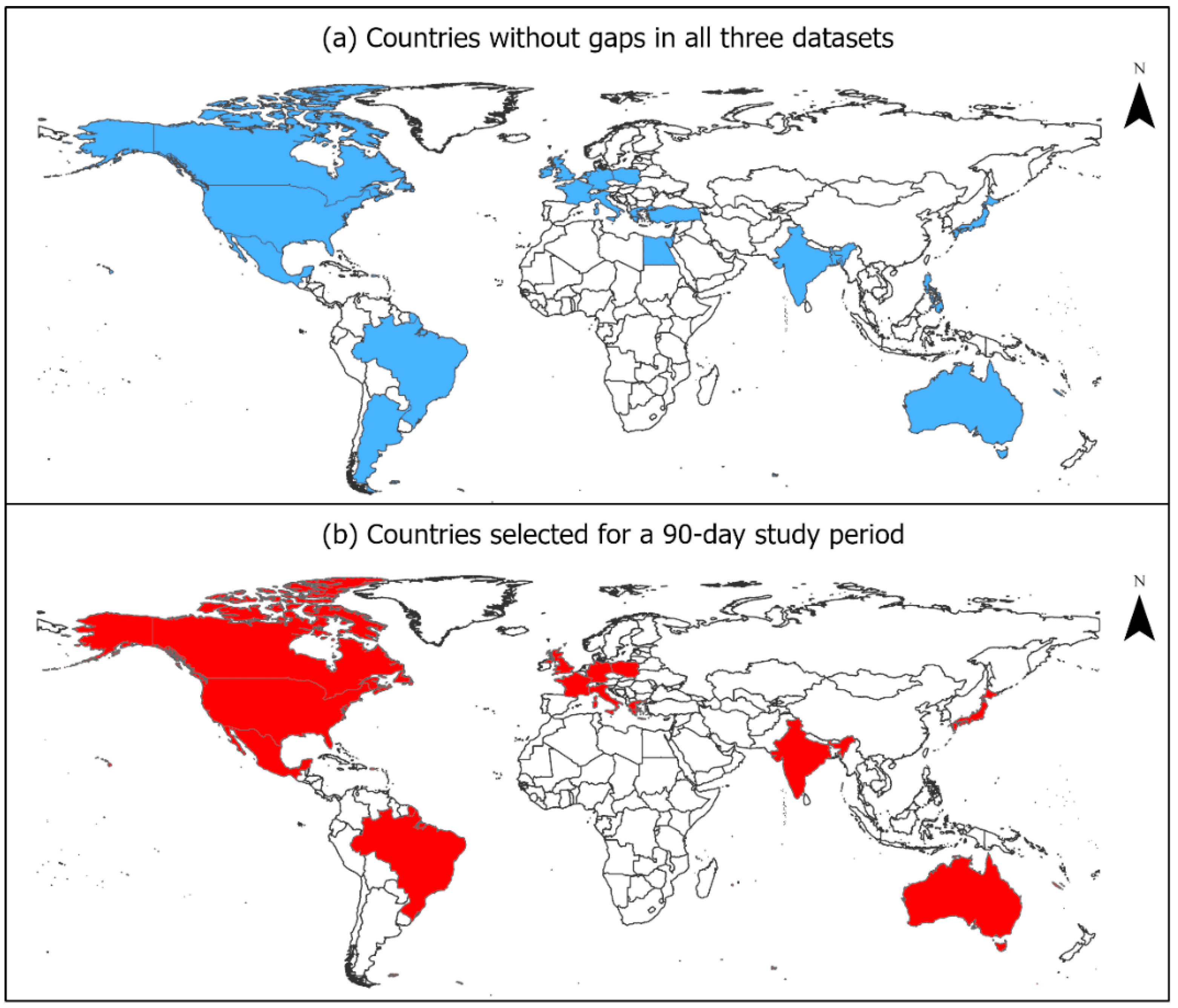
• Assess time-lagged relationships between new COVID-19 cases and the number of COVID-19-related GDELT articles and tweets in selected countries using cross-correlation analysis.
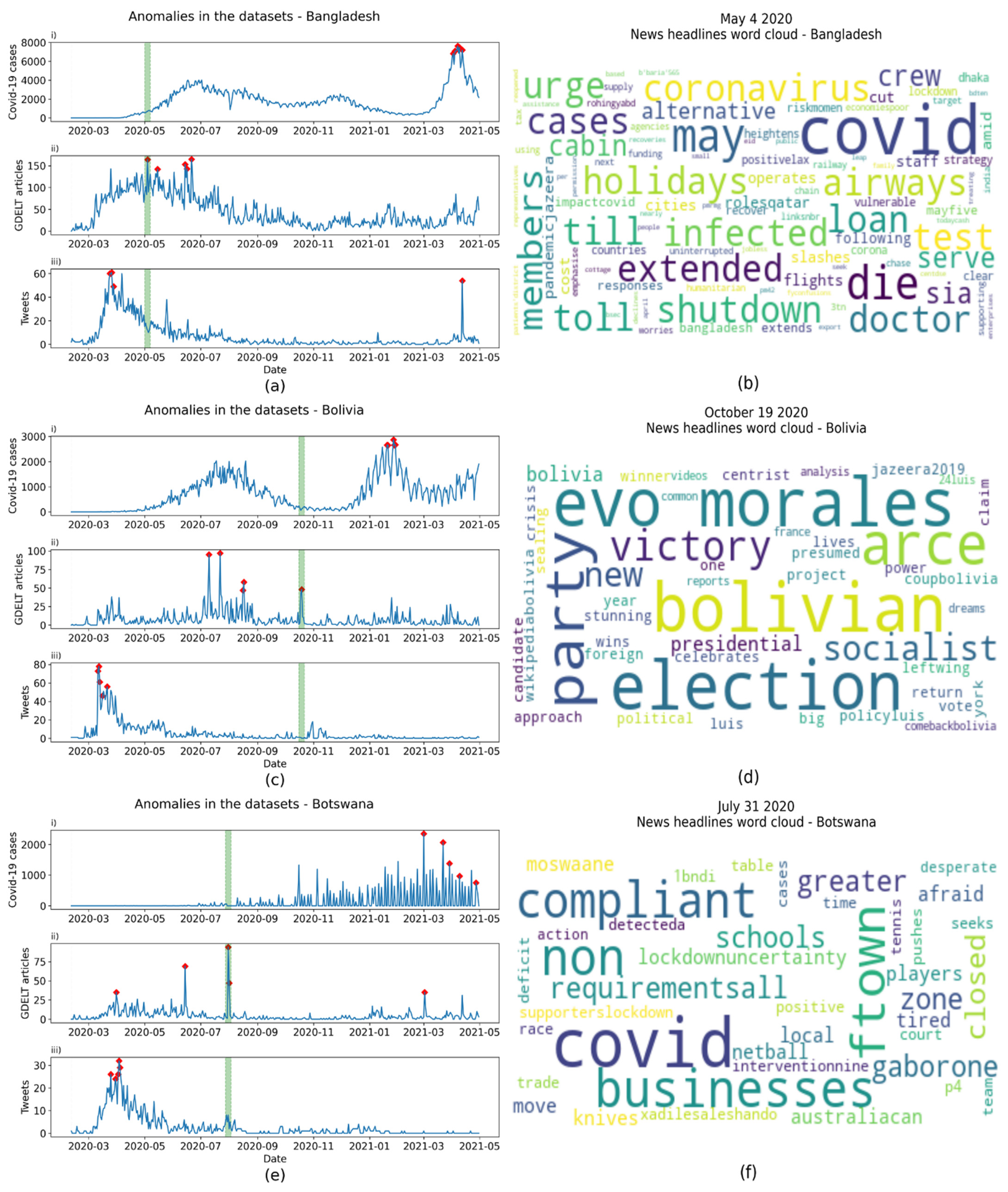
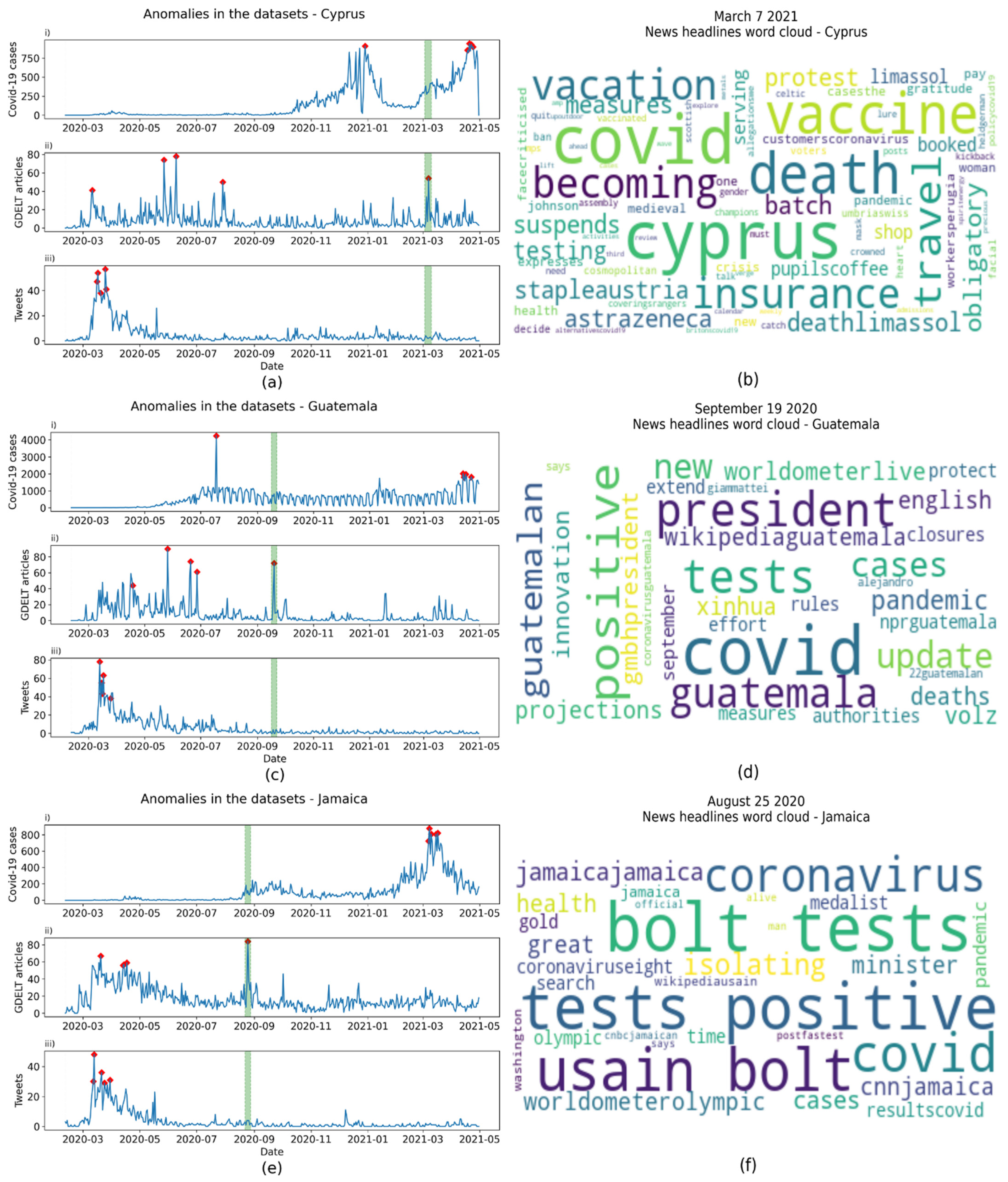
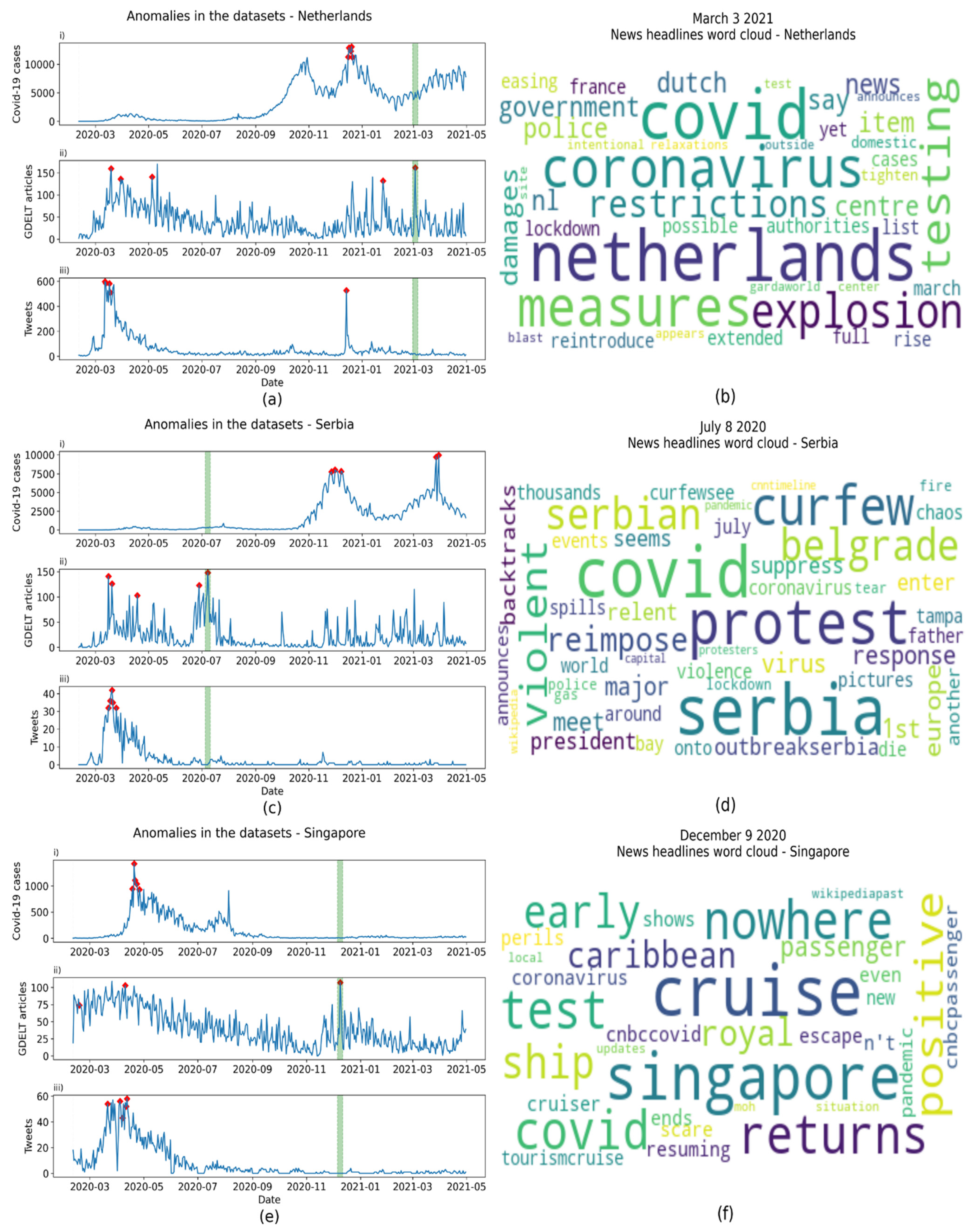
• Identify anomalies and their causes on days with abnormally high COVID-19-related responses on GDELT and Twitter but low numbers of new COVID-19 cases.

2. Literature Review

Previous studies have exemplified how social media platforms, news media portals, and data from online search engines are reflective of the chronology of real-time events [20,21]. They used time series analysis to examine pattern changes and time-lagged relationships and to make predictions.

Time-lagged relationships between time series datasets are often determined using cross-correlation analysis [18]. At the core of the method is the use of an autoregressive integrated moving average (ARIMA) model, where future values of a univariate time series with a constant mean and variance are predicted using its past values and errors of the series [22]. In the case of existing feedback relationships, where the predictor and the dependent variables influence each other, vector autoregressive (VAR) models are more appropriate [23].

Cross-correlation analysis has been used to study the temporal relationship between factual information and misinformation related to COVID-19 on Twitter [24] as well as the effect of various climate variables, such as solar exposure, on the spread of COVID-19. It has also been used to explore the interaction between social media posts (tweets), traditional mass media outlets (newspapers), and information-seeking tools (Google Trends) during peak years of the California drought 2013–2015 [25]. Regarding GDELT, cross-correlation analysis revealed that the Saudi Stock Market Index (TASI) lagged the tone of GDELT news by one day, indicating that GDELT could have a predictive power over TASI [26].

Regular patterns in a time series can be affected by other events, leading to abnormal changes. Such artifacts can be discovered through a variety of methods, which can be categorized into statistical, clustering, classification, and regression techniques [27]. Time series data from online sources tend to exhibit characteristics such as multimodal distribution, volatility, and seasonality, which need to be handled accordingly in anomaly detection, for example, by using the seasonal hybrid extreme Studentized deviate (SHESD) test [28]. This method has been applied in the temporal analysis of Twitter data and Google Trends before [29] and is a modified version of the extreme Studentized deviate (ESD) test [30].

Social media data have known limitations such as geodata sparsity, retrieval restrictions, and sociodemographic bias, and they are affected by data privacy regulations [13]. GDELT’s global coverage of events with over two billion geocoded data, its historical coverage which reaches back to 1979, and its 15 min update cycle allow for a comprehensive and rapid analysis of events. These facts render GDELT a potentially viable alternative data source to Twitter and other social media for disease monitoring and prediction. GDELT has been rarely used in the context of COVID-19, with only a few exceptions, such as the use of 4Chan, Reddit, and GDELT data to analyze pandemic-related conspiracies [31].

Existing studies have analyzed online news media coverage of COVID-19 [32] and used data from Twitter for predicting COVID-19 infections [33,34]. The spike in tweets around disease news can, among other factors, be explained by preference of user-generated content sites compared to those of governmental authorities to share disease-related news, such as information on outbreaks and case reports [35]. This can lead the number of disease-related tweets to increase even before governmental official announcements of first probable disease cases, as was found for the Ebola outbreak in Nigeria [36]. However, the accuracy of social media surveillance systems can decline with media attention, since this increases messages about the disease that do not pertain to an actual infection [37].

3. Materials and Methods

3.1. Data Sources

3.1.1. New Daily COVID-19 Infections

The number of new daily cases of COVID-19 per country reported between 11 February 2020 and 30 April 2021 were obtained as CSV files from Johns Hopkins University [38]. The data quality differs between countries due to varying degrees of access to resources needed to adequately monitor disease spread [39]. Low quality of data (e.g., missing records) for numerous countries prevented the use of their data in cross-correlation and anomaly analysis. Where possible, linear interpolation was used to fill in data gaps.

3.1.2. Twitter

The academic research product track on the Twitter API provided free access to the full-archive search endpoint. This enabled the retrieval of geotagged COVID-19-related tweets worldwide between 11 February 2020 and 30 April 2021. With an API rate limit of 900 requests/15 min, a delay between requests was used to adhere to this restriction, which extended the data collection process to seven weeks. The following ten COVID-19-related hashtags were used as a filter: #Coronavirus, #COVID2019, #2019nCoV, #COVID_19, #socialdistancing, #novelcoronavirus, #stayhome, #SARSCoV2, #lockdown, and #quarantine.

Tweets can be tagged with location data including the exact geographic coordinates or the bounding box enclosing a place (e.g., neighborhood, city, administrative area). Since Twitter for iPhone, Twitter for Android, and Instagram have the highest number of geotagged tweets and effectively exclude automated tweets (bots) [40], only tweets posted from those sources were used. Duplicate tweets shared by the same user in a day were deleted as they are characteristics of robotic content which can skew the analysis results [41]. Tweets were downloaded in JSON (JavaScript Object Notation) format and stored in a PostgreSQL database.

3.1.3. GDELT

GDELT is a worldwide news repository of events gathered from broadcast, print, and online news media in over 100 languages that contains hyperlinks to news articles. The dataset can be freely accessed as raw CSV files or, as was performed in this study, through Google BigQuery by querying GDELT’s Global Geographic Graph (GGG), which contains over 2.1 billion location mentions of events from various web news sources worldwide. The graph enables mapping of an event of interest at the location at which it is mentioned with the spatial resolution of location data extracted from articles coded as follows: 1 = country, 2 = U.S. state, 3 = U.S. city or landmark, 4 = city or landmark outside the U.S., and 5 = administrative area outside the U.S. that is equivalent to a U.S. state.

The GGG was queried to analyze the worldwide news coverage of the coronavirus pandemic between 11 February 2020 and 30 April 2021 for all five spatial resolution categories. Contextual texts like ‘COVID’ and ‘coronavirus’ were used as keywords to retrieve articles using Structured Query Language (SQL).

3.2. Data Preprocessing

For objective 1, the analysis of time series data required the extraction of underlying patterns comprising a trend, seasonality, and residuals. Preliminary analysis of the three datasets (new daily COVID-19 infections, GDELT news, and tweets) for some countries revealed a weekly seasonality pattern which can be studied using the seasonal-trend decomposition (STL) using LOESS (locally estimated scatterplot smoothing) [42]. Cross-correlation employs STL, which uses a logarithm transformation to ensure seasonal variations are constant in scale. Due to the use of a logarithm, only countries with positive count values in the three datasets between the date of the first reported COVID-19 case and 30 April 2021 were selected for cross-correlation analysis. This criterion was met by 21 out of 197 countries (Figure 1a).

Cross-correlation analysis requires each of the three datasets to be stationary, which means that their mean and variance have to be constant with no autocorrelation in the ARIMA model residuals throughout their respective timelines [23]. Therefore, time series data from each of the 21 previously identified countries were screened for the presence of a 90-day period which satisfied required statistical regularities in each of the three datasets. Such a 90-day period was identified for a subset of 13 countries (Figure 1b).

As a result, cross-correlations between COVID-19 cases and related GDELT articles and tweets were computed for a 12-week period between 29 February 2020 and 29 May 2020 for Australia, Canada, Germany, Italy, the U.K., and the U.S., and between 11 March 2020 and 9 June 2020 for France, Brazil, Greece, India, Philippines, Poland, and Mexico.

For objective 2, anomaly detection and text analysis were attempted on the three datasets for the original 197 countries between 11 February 2020 and 30 April 2021. Datasets from numerous countries had to be excluded from the analysis because of low daily sample numbers in any of the three sources. This left the following ten countries for this part of the analysis: Bangladesh, Bolivia, Botswana, Cyprus, Guatemala, Jamaica, Lebanon, Netherlands, Serbia, and Singapore.

For the 23 countries analyzed for objective 1 (13 countries) and objective 2 (10 countries), a weekly average of 1,514,844 new COVID-19 cases, 23,901 related tweets, and 48,958 related GDELT news mentions were observed.

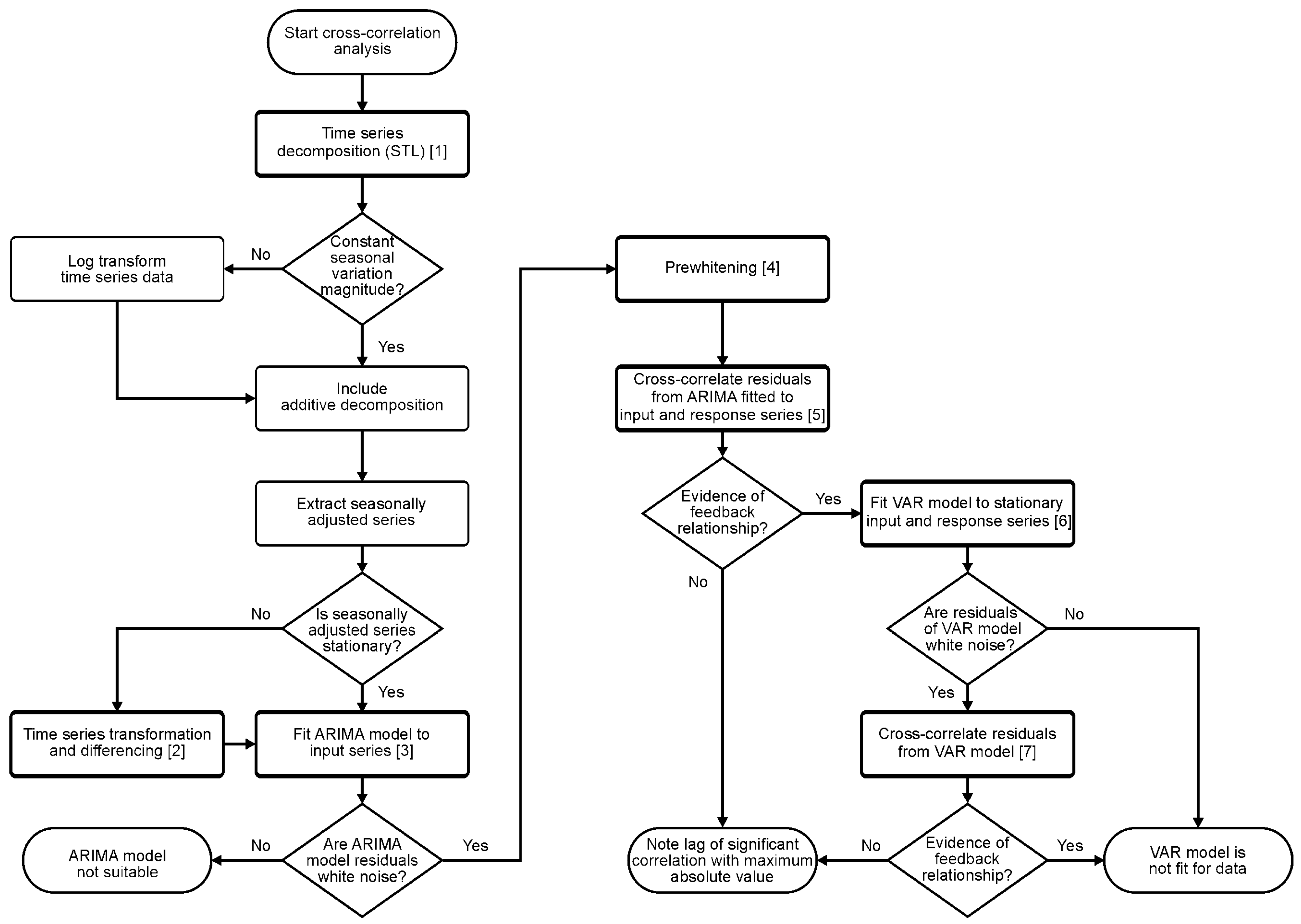
3.3. Cross-Correlation Analysis

Cross-correlation analysis models the time-lag relationship between two time series datasets by measuring their similarity through the correlation coefficient at each lag and testing its significance. The time series of the independent variable (new COVID-19 infections) is the input series, whereas the dependent variable (GDELT articles or tweets) is the response series. The principle of cross-correlation entails carrying out a lagged regression where the response time series (Y variable) is predicted at the present time using lags of an input times series (X variable) and lags of the Y variable.

This process cannot be performed using the original time series datasets because the cross-correlation function (CCF) value is affected by the time series structure of the input series and any long-term common patterns between the input and response series, which results in dependencies [43]. These interdependencies can be removed through prewhitening. During this procedure, an ARIMA model is first fitted to the input series (COVID-19 cases), and then the same model is fitted to the response variable (GDELT/Twitter). Finally, their respective residuals are used to calculate the CCF. Prewhitening helped, for example, to remove dubious correlations resulting from chronological dependencies between COVID-19 cases and related GDELT articles or tweets [31].

The steps involved in cross-correlation analysis are described in the following subsections and annotated through numbers in the flowchart (Figure 2) as follows: (1) time series decomposition, (2) transformation and differencing, (3) ARIMA model fitting, (4) prewhitening, (5) cross-correlation of residuals from the ARIMA model, (6) vector autoregressive model fitting, and (7) cross-correlation of residuals from the VAR model.

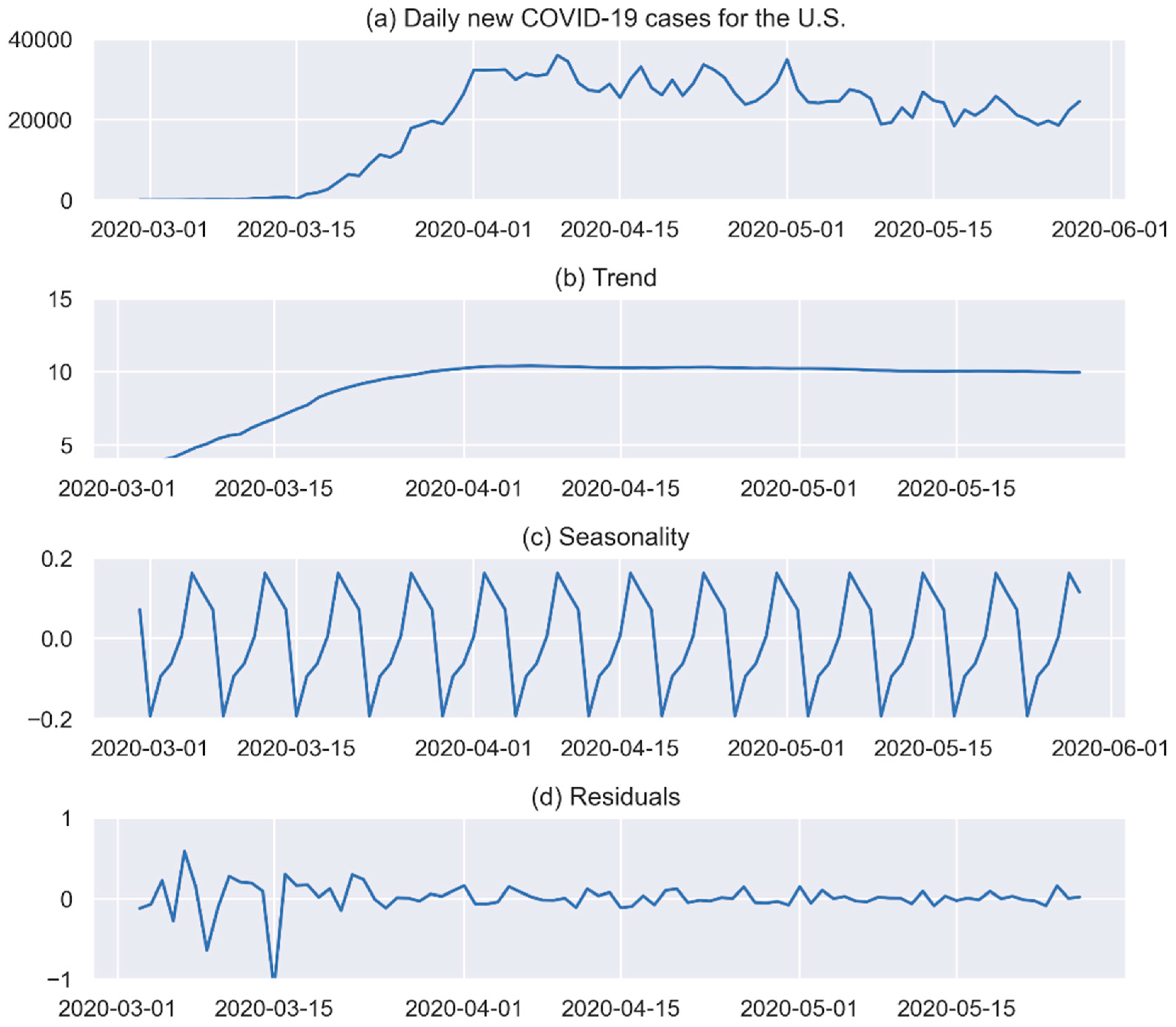
3.3.1. Step 1: Time Series Decomposition

The patterns inherent in each of the three time series datasets (new COVID-19 cases, GDELT activity, and Twitter activity) can be split into three components, i.e., trend, seasonality, and residuals. This is shown in Figure 3b–d for new COVID-19 cases for the U.S. as an example.

During the decomposition process of time series data, components can be combined additively or multiplicatively, reflecting an additive or multiplicative decomposition approach, respectively. Additive decomposition is applicable when the magnitude of the seasonal component fluctuations is constant over time, whereas multiplicative is used when it changes over time.

The trend, which is the upward or downward pattern of a time series, can be estimated using smoothing techniques such as moving average. Seasonality expresses fluctuations that occur repeatedly after specific periods. A fast Fourier transform (FFT) applied to COVID-19 case numbers, GDELT news articles, and tweets time series data revealed a predominant frequency of seven days and, thus, a weekly seasonality. Removal of seasonality and trend is a prerequisite for achieving stationarity before cross-correlation [44].

The residuals are the noise components which remain after the removal of trend and seasonal parts. They can be distorted by large anomalies, which affect the mean and exaggerate the variance of time series data values. This influence can be reduced through the STL technique, which uses locally weighted regression to extract the seasonal component. Each of the three time series datasets for the remaining 13 countries were of a multiplicative nature and hence were decomposed using R (stl function in the R stats package) into their constituent parts. The seasonally adjusted data were recovered by applying R (seasadj function in the R forecast package) on the decomposed components to remove the seasonal components.

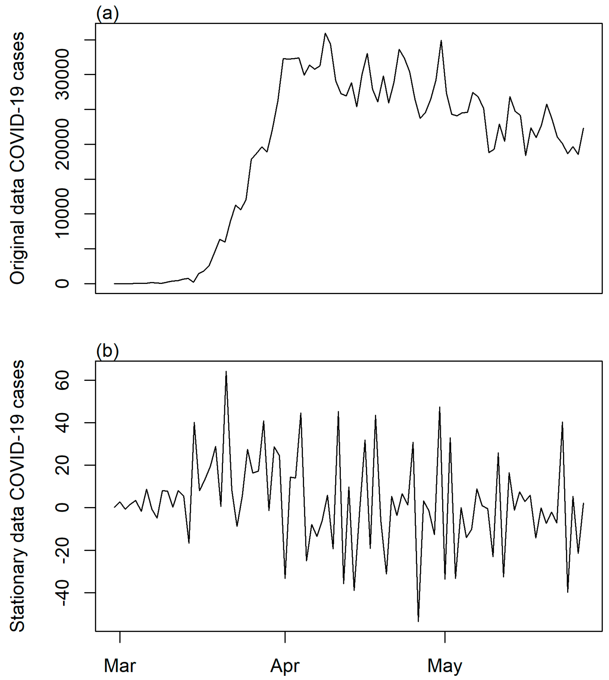
3.3.2. Step 2: Time Series Transformation and Differencing

The augmented Dickey–Fuller (ADF) test showed that seasonally adjusted observations of the three datasets for the 13 countries were nonstationary. To reach a stable variance, a power transformation (Equation (1), upper clause) was applied to each variable ${\mathrm{y}}_{\mathrm{t}}$ $\mathrm{a}\mathrm{t}$ a time period t where lambda λ values were chosen from the interval [0; 1] using R (BoxCox.lambda function in the R forecast package). If λ = 0, Box–Cox transformations [45] can be applied instead (Equation (1), lower clause).

$${\mathrm{w}}_{\mathrm{t} }=\left\{\begin{array}{c}{(\mathrm{y}}_{\mathrm{t} }^{\mathsf{\lambda }}-1)/\mathsf{\lambda }\hspace{1em}\mathrm{if} \mathsf{\lambda } \ne 0.\\ \mathrm{l}\mathrm{o}\mathrm{g}{(\mathrm{y}}_{\mathrm{t}}) \hspace{1em}\mathrm{if} \mathsf{\lambda } = 0;\end{array}\right.$$

(1)

To stabilize the mean and remove the trend, the transformed datasets underwent first-order differencing. Figure 4a depicts the original U.S. COVID-19 cases time series between 29 February 2020 and 29 May 2020, and Figure 4b shows the result of these two processes (transformation and differencing). A subsequent ADF test confirmed that the modified time series were stationary.

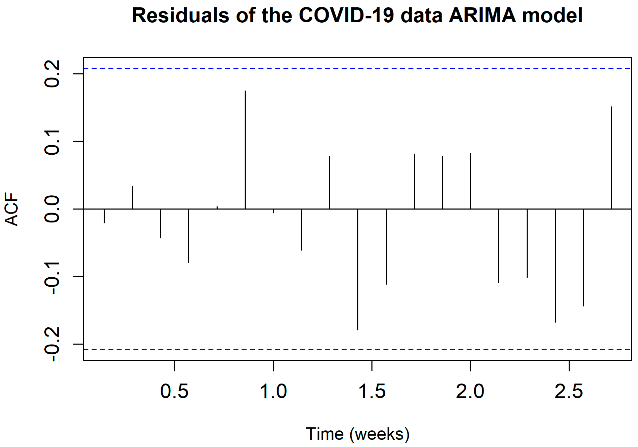
3.3.3. Step 3: Fitting an ARIMA Model to the Input Series

An ARIMA model performs time series forecasts using its past data values, which are defined in the autoregressive (AR) term, and past errors, which are described by the moving average (MA) term. The (I) term represents the order of differencing applied.

An ARIMA model specification is given as ARIMA (p, d, q) where p captures the AR term, d the differencing order, and q the MA term. With a seasonal component present, additional (P, D, Q)_s terms are included where P, D, Q, and s represent the seasonal AR term, differencing order, MA term, and seasonality, respectively, as in ARIMA (p, d, q) (P, D, Q)_s. An ARMA (autoregressive moving average) model of (p, q) order consists of p AR and q MA terms, as shown in Equation (2) where $\left\{{\mathrm{Z}}_{\mathrm{t}}\right\}$ is a purely random process with mean zero and variance ${\mathsf{\sigma }}_{\mathrm{z}}^2$ and ${\mathsf{\alpha }}_{1\dots \mathrm{p}}$ and ${\mathsf{\beta }}_{1\dots \mathrm{q}}$ are the autoregressive and moving average coefficients, respectively [46].

$${\mathrm{X}}_{\mathrm{t}}={\mathsf{\alpha }}_1{\mathrm{X}}_{\mathrm{t}-1}+\dots +{\mathsf{\alpha }}_{\mathrm{p}}{\mathrm{X}}_{\mathrm{t}-\mathrm{p}}+{\mathrm{Z}}_{\mathrm{t} }+{\mathsf{\beta }}_1{\mathrm{Z}}_{\mathrm{t}-1}+\dots +{\mathsf{\beta }}_{\mathrm{q}}{\mathrm{Z}}_{\mathrm{t}-\mathrm{q}}$$

(2)

${\mathrm{X}}_{\mathrm{t}}$ represents a time series variable at time t estimated through a linear combination of the lagged values (${\mathrm{X}}_{\mathrm{t}-1}$...${\mathrm{X}}_{\mathrm{t}-\mathrm{p}}$) of ${\mathrm{X}}_{\mathrm{t}}$ where p are the lags of the AR terms and ${\mathrm{Z}}_{\mathrm{t}-1}$...${\mathrm{Z}}_{\mathrm{t}-\mathrm{q}}$ represent lagged forecast errors in past values with q as the lags of the MA terms.

Using the backward shift operator B, Equation (2) can be rewritten as (Equation (3)):

$$\mathrm{ARMA}\left(\mathrm{p},\mathrm{q}\right):\mathsf{\varphi }\left(\mathrm{B}\right){\mathrm{X}}_{\mathrm{t}}=\mathsf{\theta }\left(\mathrm{B}\right){\mathrm{Z}}_{\mathrm{t}}$$

(3)

where ϕ is a nonseasonal autoregressive parameter of order p, θ a nonseasonal moving average parameter of order q, and ϕ(B) and θ(B) polynomials of order p, q, respectively, such that (Equation (4))

$$\mathsf{\varphi }\left(\mathrm{B}\right)=1-{\mathsf{\alpha }}_1\mathrm{B}-\dots -{\mathsf{\alpha }}_{\mathrm{P}}{\mathrm{B}}^{\mathrm{P}}$$

(4)

$$\mathsf{\theta }\left(\mathrm{B}\right)=1+{\mathsf{\beta }}_1\mathrm{B}+\dots +{\mathsf{\beta }}_{\mathrm{q}}{\mathrm{B}}^{\mathrm{q}}$$

ARIMA adds a nonseasonal differencing order d with (1 − B)^d equal to the d-th nonseasonal difference so that an ARIMA process of order (p, d, q) can be formulated as (Equation (5)):

$$\mathrm{ARIMA}\left(\mathrm{p},\mathrm{d},\mathrm{q}\right):\mathsf{\varphi }\left(\mathrm{B}\right){(1-\mathrm{B})}^{\mathrm{d}}{\mathrm{X}}_{\mathrm{t}}=\mathsf{\theta }\left(\mathrm{B}\right){\mathrm{Z}}_{\mathrm{t}}$$

(5)

After obtaining stationarity in the daily COVID-19 dataset, it was fitted to an ARIMA model using R (auto.arima function in the R forecast package) to identify the best ARIMA model based on the Akaike information criterion (AIC) [47].

The residuals were normally distributed, had a zero mean and constant variance, and were not autocorrelated, as confirmed using R (checkresiduals function in the R forecast package). The function includes the Ljung Box test [48], which tests the overall randomness based on a number of lags. The test resulted in a correlogram, which plots residual autocorrelation function values (ACF) against lag time (Figure 5). All lags fall inside the 95% confidence interval (dashed blue lines), indicating that the residuals from the ARIMA model for new COVID-19 cases in the U.S. were not autocorrelated.

3.3.4. Steps 4 and 5: Prewhitening and Cross-Correlation of Residuals

The ARIMA (0, 1, 2) (1, 0, 1)₇ model for the U.S. obtained in the previous step was fitted to the stationary response variables, i.e., COVID-19-related GDELT articles and tweets for the U.S., respectively (step 4). The residuals were then cross-correlated with residuals from the ARIMA model of the COVID-19 dataset (step 5). CCF plots in Figure 6 display cross-correlation values of COVID-19 cases versus GDELT articles (Figure 6a) and tweets (Figure 6b) in the U.S. for different time lags.

Qualitative aspects of cross-correlation plots from previous works [19] guided the interpretation of the cross-correlation results. This includes use of the highest peak magnitude in the plot, which indicates the strength of the correlation between the two time series at that specific time lag, as well as the arithmetic sign, which specifies the direction of strength of the peaks. The time lag at significant cross-correlations, determined through hypothesis testing at a predetermined 0.05 significance level, was used as a quantitative measure.

Each CCF plot can be divided into four quadrants representing different combinations of arithmetic signs for cross-correlations and lags. When a significant correlation is found on positive lags (x axis), it means that the GDELT or Twitter time series leads the COVID-19 time series, whereas a negative lag means the opposite. Cross-correlation patterns for analyzed countries fell into either quadrant 1 or 3, which will therefore be discussed in more detail in the Results section. The lag whose correlation value exceeds the blue dashed line and has the largest absolute value is picked as the lag for interpretation [49].

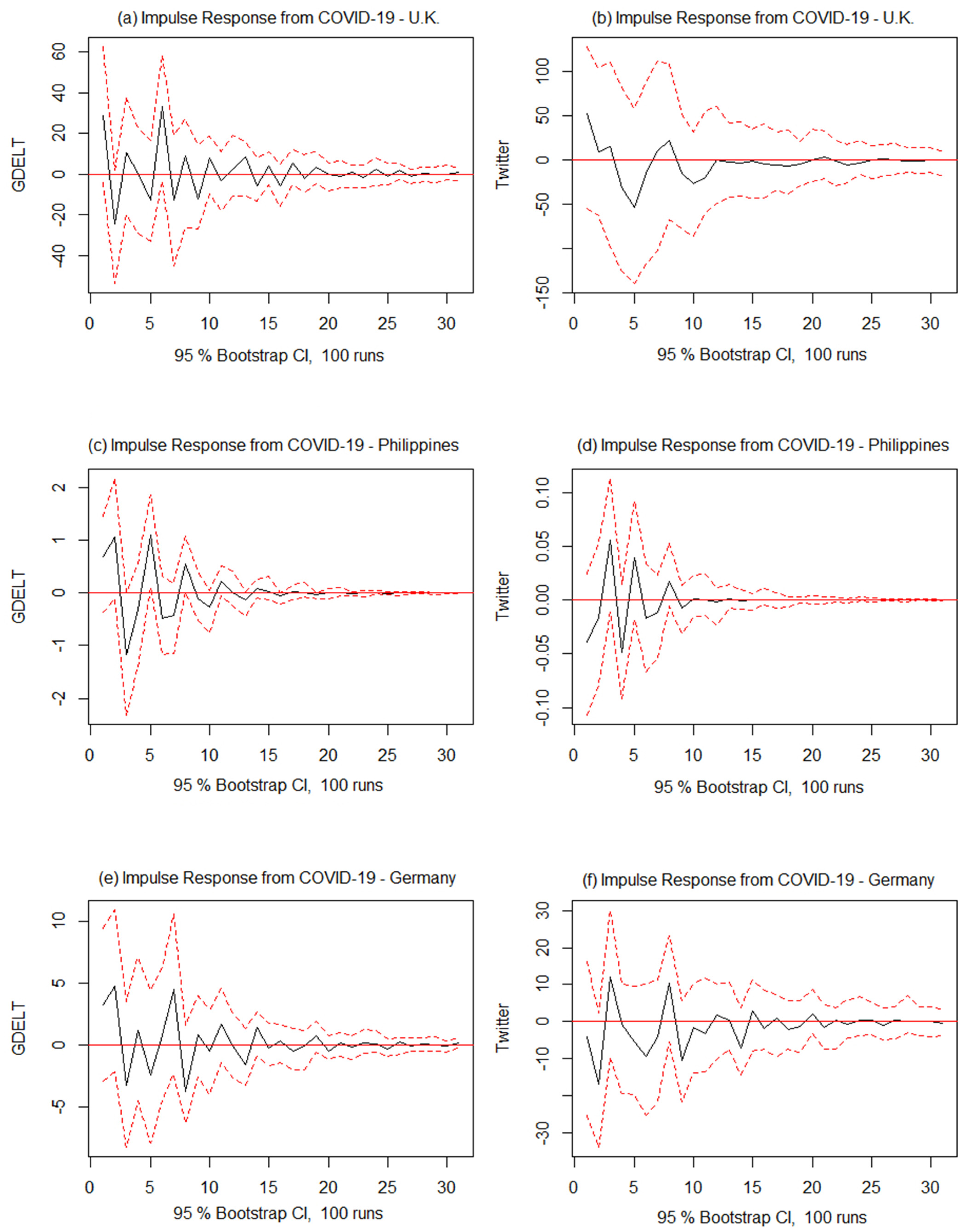
3.3.5. Steps 6 and 7: Vector Autoregressive Models and Cross-Correlation of Residuals

The cross-correlation of residuals from ARIMA models sometimes yields inconclusive results, as indicated through significant correlations in both the positive and negative lags. This occurrence shows the presence of a feedback relationship where the dependent and predictor variables influence each other. In such a case, a VAR model can help distinguish the dynamics of the interrelations between variables [23] (step 6). A VAR model requires the time series datasets to meet the stationarity condition. Therefore, time series decomposition, differencing, and transformation must be applied before the optimal VAR model can be identified based on the lowest AIC value. A useful VAR model yields uncorrelated, heteroscedastic, normally distributed, and stable residuals.

A formulation of a VAR (p) model with m variables and of p-th order can be written as (Equation (6) [46]):

$$\mathsf{\Phi }\left(\mathrm{B}\right){\mathbf{X}}_{\mathbf{t}}={\mathsf{ϵ}}_{\mathbf{t}}$$

(6)

where ${\mathbf{X}}_{\mathrm{t}}$ is an (m × 1) vector of m observed variables, Φ is a matrix polynomial of order p in the backward shift operator B, and ${\mathsf{ϵ}}_{\mathrm{t}}$ is a vector of white noise error terms for the m variables at time t. A VAR (1) model for two series is shown in Equation (7), where values of ${\mathrm{X}}_{1, \mathrm{t}}{ \mathrm{and} \mathrm{X}}_{2,\mathrm{t}}$ depend linearly on the values of both series at time t−1, and {${\mathsf{\varphi }}_{\mathrm{ij}}$} are autoregressive coefficients.

$${\mathrm{X}}_{1,\mathrm{t} }={\mathsf{\varphi }}_{11}{\mathrm{X}}_{1,\mathrm{t}-1 }+{\mathsf{\varphi }}_{12}{\mathrm{X}}_{2,\mathrm{t}-1 }+{\mathsf{ϵ}}_{1,\mathrm{t}}$$

(7)

$${\mathrm{X}}_{2,\mathrm{t} }={\mathsf{\varphi }}_{21}{\mathrm{X}}_{1,\mathrm{t}-1 }+{\mathsf{\varphi }}_{22}{\mathrm{X}}_{2,\mathrm{t}-1 }+{\mathsf{ϵ}}_{2,\mathrm{t}}$$

In the first VAR model in our study, ${\mathrm{X}}_1$ and ${\mathrm{X}}_{2 }$ represent COVID-19 cases and COVID-19-related GDELT articles, respectively, and in the second VAR model, ${\mathrm{X}}_1$ and ${\mathrm{X}}_{2 }$ represent COVID-19 cases and COVID-19-related tweets, respectively. For each VAR model, the ACF of the residuals from the variables did not have any significant correlations for any lag; thus, residuals were considered white noise. These residuals from the respective VAR model were then cross-correlated individually to find significant correlations at different lags to identify the lead–follow patterns between the variables in the model (step 7).

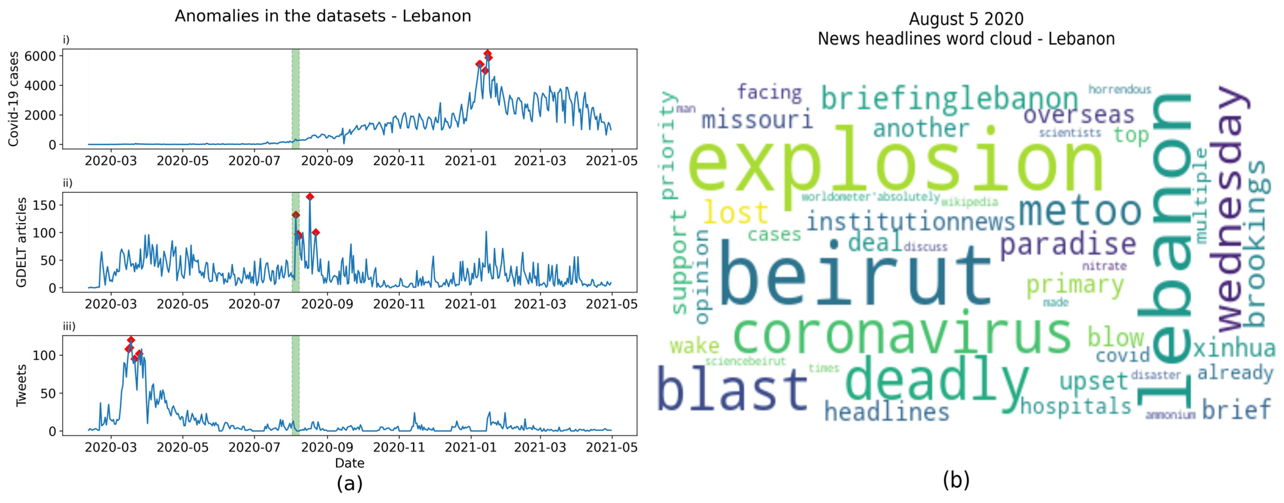
3.4. Anomaly Detection

The three analyzed datasets exhibited weekly seasonality patterns and multimodal distribution for all ten countries in this part of the study, rendering conventional anomaly detection methods such as the Grubbs’ test and extreme Studentized deviate (ESD) test, which require normally distributed data, unsuitable [30]. Therefore, the SHESD test, which is a modified version of the ESD test, was used instead to find unexpected patterns in COVID-19-related activities on GDELT and Twitter.

For the ESD test, the residual component of a time series ${\mathrm{R}}_{\mathrm{t}}$ at time t is obtained by subtracting the seasonal component ${\mathrm{S}}_{\mathrm{t}}$ and the median ${\mathrm{M}}_{\mathrm{t}}$ from the values of the original time series ${\mathrm{Y}}_{\mathrm{t} }$(Equation (8)):

$${\mathrm{R}}_{\mathrm{t} }={ \mathrm{Y}}_{\mathrm{t} }-{\mathrm{S}}_{\mathrm{t}} -{\mathrm{M}}_{\mathrm{t}}$$

(8)

The ESD test is then applied to the residuals, which requires defining an upper bound of the number of suspected outliers (k). Its null hypothesis is that there are no outliers, while the alternative hypothesis is that there are up to k outliers in the dataset. The ESD test performs k separate runs, i.e., a test for one outlier, a test for two outliers, etc., up to k outliers, with a total of k test statistics. The SHESD test is a variation of the ESD test in that it uses (a) the median in place of the mean and (b) the median of absolute deviations from the sample median in place of the standard deviation to compute the test statistics.

A comparative review of outlier detection methods found that the SHESD test performs satisfactorily in identifying point anomalies on univariate data [50], which is the setting in our study.

3.5. Word Frequency Analysis

The results from anomaly detection were used to identify events that caused a spike in the number of COVID-19-related GDELT articles and tweets during days of few newly reported COVID-19 infections. To identify potential events causing such spikes, articles for a country of interest were obtained from the NewsBank news repository [51] using the ‘COVID’ keyword. In addition, a customized Python script was used to scrape results from a Google search with search terms comprising the date of the anomaly, the country name of interest, and the word ‘COVID’.

Word frequency analysis was run on unstructured text in the headlines using the Natural Language Toolkit (NLTK) package in Python after headlines were tokenized (extraction of individual words) and stop words, such as prepositions or conjunctions, and punctuation marks were removed. High-frequency buzzwords were then visualized as word clouds using the word cloud Python library.

4. Results

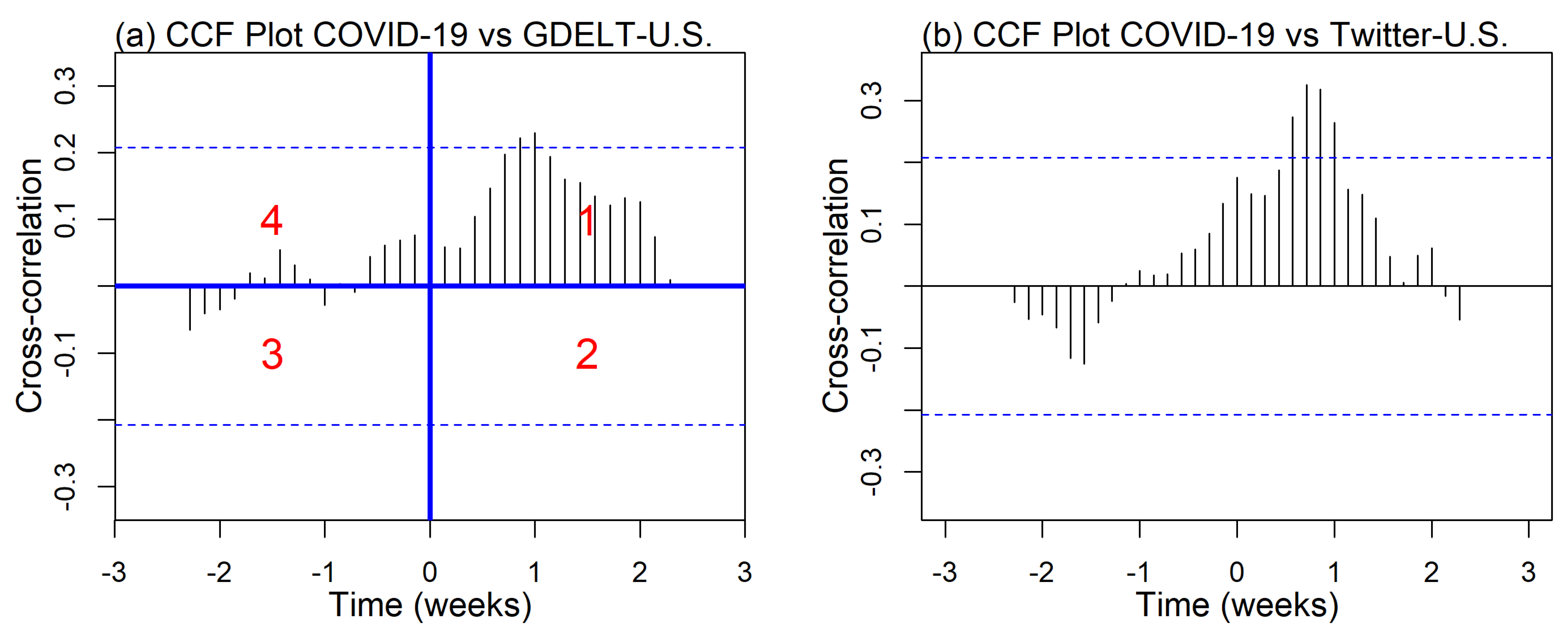
4.1. Cross-Correlation

The temporal relationships between new daily COVID-19 infections (input series) and COVID-19-related GDELT articles and tweets (output series) are depicted in cross-correlograms. The following sections discuss the 12 countries that revealed significant cross-correlation, grouped by the arithmetic sign of cross-correlation, and identified lags, i.e., by quadrants shown in Figure 6a.

4.1.1. Positive Lag

The cross-correlation of COVID-19 cases versus GDELT and Twitter had significant positive correlations on positive lags (first quadrant) for the U.S. (Figure 6), Australia, India, Brazil, Greece, and Italy. The same cross-correlation pattern (first quadrant) was reflected only for Twitter but not GDELT for France. Significant positive correlations on positive lags imply that the input series (COVID-19) follows GDELT and tweet activity numbers, respectively. The CCF plot for COVID-19 cases versus Twitter for Greece reveals a significant positive correlation at lag 0, meaning that COVID-19-related tweets reflect COVID-19 infections immediately, without lag time.

4.1.2. Negative Lag

COVID-19 cases versus GDELT CCF plots for Poland reveal a significant negative correlation at a negative lag (third quadrant). This means that the input series (new COVID-19 cases) led related GDELT articles, respectively. Therefore, as COVID-19 cases increased, the respective GDELT articles followed with a delayed decrease. The COVID-19 cases versus Twitter CCF had a significant positive correlation at lag 0 (first quadrant), meaning that COVID-19-related tweets reflected COVID-19 infections immediately, without lag time.

4.1.3. Positive and Negative Lag

In the datasets for Canada, the U.K., the Philippines, and Germany, significant correlations were found at both negative and positive lags, which is indicative of feedback relationships. For example, COVID-19 cases versus GDELT news CCF plots had significant correlations for positive and negative lags. To determine the most significant correlation and the direction of the relationship, VAR models were used instead.

After implementing separate VAR models, the cross-correlations of residuals for COVID-19 infections versus GDELT and Twitter for Canada resulted in single significant correlations on positive lags indicating that the input series (COVID-19) followed GDELT without lag time (lag 0) and tweets by 11 days, respectively. A similar application of VAR models led to single significant correlations for either negative or positive lags for GDELT and Twitter correlograms for the U.K., the Philippines, and Germany.

Estimated coefficients, standard errors, and goodness-of-fit measures for the VAR models are shown in

Table 1. VAR parameters for COVID-19 infections versus GDELT and Twitter (Canada).

Lag	VAR (COVID-19 and GDELT)		Lag	VAR (COVID-19 and Twitter)
	COVID-19	GDELT		COVID-19	Twitter
COVID-19 (1)	−0.860 *** (0.122)		COVID-19 (1)	−0.865 *** (0.22)
GDELT (1) (1)		−0.289 ** (0.121)	Twitter (1)	0.002 * (0.001)
GDELT (2)		−0.288 *** (0.125)	Twitter (2)		−0.466 *** (0.120)
GDELT (3)	0.029 * (0.015)		Twitter (3)		0.303 * (0.130)
COVID-19 (5)	0.346 ** (0.156)		Twitter (4)	0.002 * (0.001)
COVID-19 (6)	0.234 * (0.122)		Twitter (5)	2.079 ** (0.937)	0.334 *** (0.124)
N	83	83		84	84
R2	0.614	0.219		0.601	0.385
Adjusted R2	0.506	0.091		0.506	0.238

p < 0.001 ‘***’, p < 0.05 ‘**’, p < 0.1 ‘*’.

(Canada) and

Table A1. VAR parameters for COVID-19 infections versus GDELT and Twitter for the U.K., the Philippines, and Germany.

	Lag	VAR (COVID-19 vs. GDELT)		Lag	VAR (COVID-19 vs. Twitter)
		COVID-19	GDELT		COVID-19	Twitter
U.K.	GDELT (1)		−0.429 *** (0.128)	Twitter (2)		−0.546 *** (0.125)
	GDELT (2)		−0.291 ** (0.141)	Twitter (6)		0.218 * (0.126)
	COVID-19 (5)		−0.087 * (0.045)	COVID-19 (7)	0.229 ** (0.123)
	COVID-19 (7)	0.217 * (0.122)		Twitter (4)		0.213 * (0.123)
	N	82	82		82	82
	R2	0.482	0.281		0.448	0.416
	Adjusted R2	0.312	0.046		0.267	0.225
Philippines	COVID-19 (1)	−0.615 *** (0.101)	5.450 ** (2.173)	COVID-19 (1)	−0.599 *** (0.121)
	GDELT (1)		−0.448 *** (0.103)	Twitter (1)	0.191 * (0.114)	−0.594 *** (0.118)
	COVID-19 (2)	−0.475 *** (0.105)		COVID-19 (2)	−0.449 ** (0.138)
	GDELT (2)		−0.421 *** (0.098)	Twitter (2)		−0.375 * (0.132)
				Twitter (3)		−0.301 ** (0.131)
	N	87	87		82	82
	R2	0.391	0.364		0.449	0.352
	Adjusted R2	0.311	0.281		0.338	0.222
Germany	COVID-19 (1)	−0.625 *** (0.113)	0.011 ** (0.005)	COVID-19 (1)	−0.653 *** (0.125)
	GDELT (1)		−0.665 *** (0.121)	Twitter (3)	1.692 * (0.915)
	GDELT (2)		−0.513 *** (0.145)	COVID-19 (4)	0.322 ** (0.132)
	GDELT (3)		−0.430 *** (0.150)	Twitter (4)		0.213 * (0.123)
	COVID-19 (4)	0.302 ** (0.131)		COVID-19 (5)	0.443 *** (0.136)
	COVID-19 (5)	0.386 *** (0.112)		Twitter (6)	2.079 ** (0.937)
	N	84	84		82	82
	R2	0.522	0.418		0.598	0.322
	Adjusted R2	0.408	0.280		0.467	0.099

p < 0.001 ‘***’, p < 0.01 ‘**’, p < 0.05 ‘*’.

(the U.K., the Philippines, and Germany). In the VAR model that uses COVID-19 cases and GDELT responses, 50.6% of the variation in COVID-19 cases was explained by both variables at specific lags (second column). For the VAR model that uses COVID-19 cases and Twitter responses, COVID-19 cases on lag 1 and related content from Twitter at lags 1, 4, and 5 explain 50.6% of the variation in COVID-19 cases (fifth column). The VAR models explain 9.1% and 23.8% of the variation in the COVID-19-related GDELT (third column) and Twitter (sixth column) responses, respectively, using different lags. Corresponding results for the U.K., the Philippines, and Germany are presented in Table A1.

To analyze the dynamic relationship between the variables in the VAR models, the impulse response function (IRF), as implemented in R (irf function in the R vars package), was applied to the models. This resulted in plots that were jagged, as in Figure 7 (Canada) and Figure A2 (the U.K., Philippines, and Germany).

In these figures, the y axis represents the responses of GDELT and Twitter to a one-standard-deviation shock from new COVID-19 cases over time. In all IRF plots, due to sudden changes in COVID-19 cases, there are irregular fluctuations in the responses characterized by a decline followed by tapering growth that gradually diminishes until the impact returns to zero by the end of the 30-day (x axis) period.

The optimal ARIMA models, based on the lowest AIC values for the cross-correlation analysis for all countries with significant correlations, are summarized in

Table 2. ARIMA and VAR models with their respective cross-correlation time lags.

Country	Model	Time Lag in Days		Quadrant
		COVID-19 vs. GDELT	COVID-19 vs. Twitter
Australia	ARIMA (1, 0, 2)	12	3	1
Brazil	ARIMA (0, 0, 1) with nonzero mean	7	10	1
France	ARIMA (0, 0, 1)	none	8	1
Greece	ARIMA (0, 0, 1)	1	0	1
India	ARIMA (4, 0, 0) with nonzero mean	7	14	1
Italy	ARIMA (0, 1, 2) (0, 0, 1)7	16	1	1
Poland	ARIMA (2, 0, 0) with nonzero mean	−16	0	1 and 3
U.S.	ARIMA (0, 1, 2) (1, 0, 1)7	7	5	1
Canada	VAR (6)—COVID-19 and GDELT VAR (5)—COVID-19 and Twitter	0	11	1
Germany	VAR (5)—COVID-19 and GDELT VAR (7)—COVID-19 and Twitter	7	11	1
Philippines	VAR (2)—COVID-19 and GDELT VAR (4)—COVID-19 and Twitter	−7	4	1 and 3
U.K.	VAR (7)—COVID-19 and GDELT VAR (7)—COVID-19 and Twitter	15	13	1

. Only ARIMA models for the U.S. and Italy had both nonseasonal and seasonal components (weekly seasonality represented by 7), whereas the others had only nonseasonal components. Some countries, such as India, had a nonzero value of the intercept in the ARIMA model. VAR(n) models, where n stands for the autoregressive order, were applied for four countries (Canada, Germany, the Philippines, and the U.K.). No significant cross-correlations were found for Mexico.

4.2. Anomaly Detection

COVID-19, GDELT, and Twitter time series were analyzed for anomalies for ten countries (see Section 3.2). Between 11 February 2020 and 4 March 2020, most countries experienced low COVID-19 infections but high related activity on GDELT and Twitter due to the news about the virus spreading. Therefore, only outliers detected after this period were investigated.

Generally, there was a significant drop in the number of COVID-19-related tweets for all countries after May 2020. The Twitter time series, therefore, had only a few outliers after May 2020, all of which occurred when there was an upsurge in COVID-19 infection cases. This was, for example, the case for Bangladesh (Figure A3a(iii)) and the Netherlands (Figure A5a(iii)). Therefore, the anomalies that were investigated further for event detection were flagged on GDELT time series charts when COVID-19 cases were low, whereas no further investigation was conducted for tweets in this regard.

As an example, Figure 8a(ii) indicates that GDELT articles in Lebanon had an uptick on 5 August 2020 (green highlighted area) with one outlier. This was associated with keywords such as ‘explosion’, ‘deadly’, and ‘beirut’ (Figure 8b), which relate to headlines about the Port of Beirut explosion. Other GDELT anomalies on August 8, 17, and 22 (Figure 8a(ii)) were about how the blast affected the spread of infections.

The locations of COVID-19 news mentions on GDELT related to the Port of Beirut explosion in Lebanon on August 5, 2020, are mapped in Figure A1. Whereas only 209 news mentions focused on the blast, 747 news announcements mentioned the explosion in the context of COVID-19.

The GDELT outlier and word frequency analyses were able to identify at least one event in each of the ten countries (

Table 3. Buzzwords in word clouds for ten countries based on GDELT time series anomalies.

Country	Anomaly Date	Frequent Words	Events
Bangladesh	2020-05-04	holidays	National holiday
Bolivia	2020-10-19	election, party, victory	General elections
Botswana	2020-7-31	requirements, compliant	Introduction of lockdown
Cyprus	2021-03-07	Cyprus, protest	Protests
Guatemala	2020-09-19	president	President of Guatemala contracted COVID-19
Jamaica	2020-08-25	Usain Bolt	Jamaican Olympian contracted COVID-19
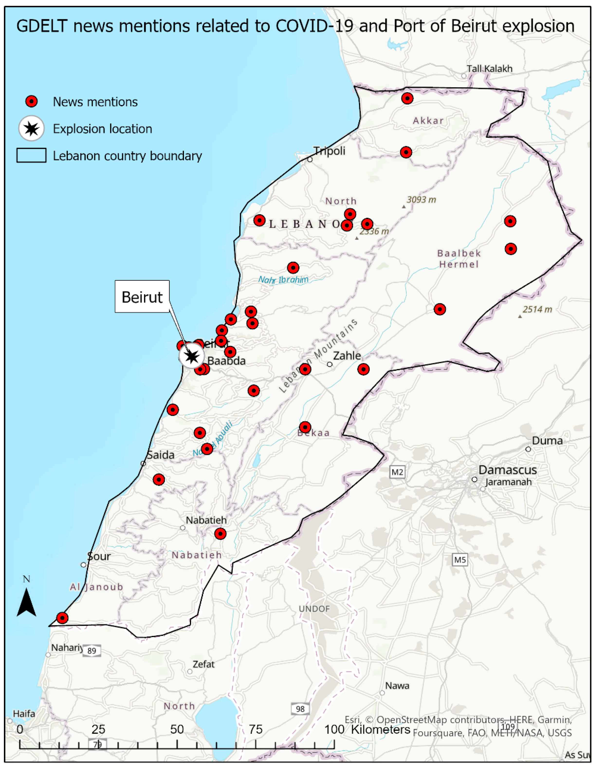
Lebanon	2020-08-05	explosion, deadly, Beirut	Beirut port explosion
Netherlands	2021-03-03	explosion	Explosion
Serbia	2020-07-08	protest, violent	Protests
Singapore	2020-12-09	cruise	COVID-19 scare on a cruise ship

). The corresponding headline buzzwords in word clouds (Figure A3 through Figure A5) describe different events discovered in the remaining nine countries, which include explosions, an election, protests, contraction of COVID-19 by prominent people, the announcement of COVID-19 mitigation measures, and a COVID-19 scare on a cruise ship.

5. Discussion

Earlier studies found that COVID-19-related Twitter posts preceded COVID-19 cases and deaths by two to three weeks [52]. Regarding the Ebola virus disease, an increase in related tweets occurred seven days prior to the confirmation of the first case of the virus [36]. In our study, ARIMA and VAR models identified similar patterns for selected countries. That is, COVID-19-related GDELT articles and tweets preceded the number of new COVID-19 infections in Australia, Brazil, Greece, India, Italy, the U.S., Canada, Germany, and the U.K., and the same was true for tweets in France, Poland, and the Philippines.

Positive cross-correlations with positive lags between COVID-19 cases and GDELT and Twitter news counts for 10 out of 12 countries (Table 2) indicate that an increase in COVID-19-related GDELT and Twitter responses was followed by an increase in new COVID-19 cases sometime later, which is in line with previous epidemiological studies [53]. COVID-19 disease incidence and Twitter activity has been found to be positively correlated in previous research [54,55,56], supporting the idea that social media is useful for disease surveillance [57]. Similarly, COVID-19 infections were also found to be positively correlated with related news reports during the start of the outbreak in China [58]. COVID-19-linked GDELT articles for Canada and tweets for Greece and Poland had instantaneous response to reports of new COVID-19 infections without lag time, which provides further evidence that online data sources can be useful for near-real-time disease monitoring [59].

Social media applications and news media have been critical for communication between officials and the public during the COVID-19 pandemic to share public health information and mitigate the spread of the virus [43]. Our study theorizes that the findings of COVID-19-linked GDELT articles and tweets preceding reports of COVID-19 infections are an indicator of how news media and social media were globally used to encourage the public to take preventative action to mitigate disease spread.

For Poland and the Philippines, the CCF results show that COVID-19-related GDELT responses lagged behind new infections and were negatively correlated to each other, meaning that an increase in new COVID-19 cases was followed by a decrease in related GDELT and Twitter responses after a period of time. Improvement of testing modalities (higher detection rate) and accessibility of COVID-19 tests as the pandemic progressed could have resulted in these patterns [60]. In addition, time series charts show how interest in COVID-19 dropped after May 2020 on GDELT for most countries. This drop in public attention to COVID-19 marked by lower volume counts of news items as the outbreak progressed may have led to these negative correlations as well [58]. The lack of effective treatments at the start of the pandemic caused an increase in false information about treatment and prevention measures in various online news sources and social media platforms [61]. This may have led to an inflation in COVID-19-related GDELT articles and tweets. Data breaches in social media platforms have prompted the enactment of laws and regulations such as the European Union’s General Data Protection Regulation (GDPR) in 2018. Recently, several U.S. states, such as California and New York, have passed laws to safeguard user data. These laws led some social media applications such as Facebook to restrict access to their user data through their API [62]. Our study revealed that sparsity of geotagged COVID-19 tweets was the main caveat of using Twitter data for time series analysis for various countries. A change in the Twitter app functionality in 2019 which limits users to sharing their precise locations only through the camera app led to fewer tweets with exact coordinates, which affects the sample size available for research [63]. These limitations call for the exploration of alternative data sources such as GDELT, which are not affected by data privacy regulations or changed app functionality.

Disease surveillance and prediction have often relied on reactions on social media [64] applications which result in positive correlations with the disease incidence. Cross-correlation analysis has been used to explore the causal relationships between Twitter activity and new COVID-19 cases [65]. However, the application of GDELT data in this context is underexplored. Twitter provides paid access to all tweets published since its inception in 2006 through the full-archive search API, while GDELT’s freely accessible archive currently goes back to 1979. Whereas Twitter is banned in countries such as China, pairing Twitter data with GDELT, which has a global coverage of data points, presents an opportunity to obtain a more holistic picture about the pandemic compared to one data source alone.

Multiplatform analyses using datasets such as Google search query, Wikipedia, and Twitter data to detect COVID-19 deaths have been found to be useful when conducting disease surveillance, as they provide comparative insights in relation to the research question [66]. Our study, therefore, posits GDELT as a reliable data source for this type of application, as it compares and validates its findings with those from Twitter. For instance, there was an evident drop in the volume of COVID-19-related GDELT and Twitter responses after May 2020. Since activity on social media data sources can be used as a proxy for disease activity [55], this drop can be an indicator of changes in disease risk perception by the public, which should be considered when creating pandemic control responses. In our study, GDELT data also detected a larger number of COVID-19-related local events (e.g., protests) that triggered anomalies in the respective GDELT time series charts, which shows its ability to uncover patterns that can broaden our understanding of COVID-19-related public attention beyond social media.

The lead–lag relationships observed between COVID-19-related GDELT and Twitter responses and COVID-19 cases serve as indicators of public awareness about the virus and can guide the design of targeted health communication campaigns that will sustain this awareness. In addition, the impulse response function plots of VAR models showed the dynamics of the relationship between COVID-19 cases and related GDELT and Twitter responses, which depicted the attenuation of public attention from both sources as COVID-19 cases became more commonplace. By capitalizing on the dynamics of attention, public health advisories can be timed to coincide with increased GDELT and tweet activity to ensure critical information reaches the public before the initial attention to the outbreak subsides.

Utilizing longitudinal analysis to detect anomalies within the datasets enabled the identification of pandemic-related events, which provides insights into how public discourse responds to external stimuli (e.g., holidays, disasters, and contraction of COVID-19 by prominent people).

The use of different 90-day time periods for the cross-correlation analysis means that its results are only valid for the period considered. As these temporal relationships change over time due to evolving public perceptions or media coverage, long-term forecasting using the results might be inaccurate. For longer study periods, prediction models can introduce lagged variables that capture lead–lag relationships for improved forecasting.

ARIMA and VAR models used in this study are linear models, which cannot analyze nonlinear patterns that might be present in the three datasets for other periods. In this study, deficiencies (reporting delays, data entry errors) associated with the data collection of COVID-19 cases [39] combined with the digital divide [67] can result in a skewed representation of a phenomenon and consequently affect data samples. Another aspect that may affect our cross-correlation results is that some COVID-19-related GDELT news articles or tweets observed in a country may not always relate to local cases but to events or new COVID-19 outbreaks abroad.

6. Conclusions

This study explored GDELT as an alternative data source to tweets for global disease surveillance. The combination of GDELT and Twitter data sources underscores the nuanced insights that can be unveiled regarding lead–follow patterns between online mentions and new COVID-19 cases. This study was able to capture the temporal relationship between new COVID-19 infections and GDELT/Twitter responses for 12 countries by providing both the strength and direction of their respective cross-correlations through specifying the lead–lag relationships. The results demonstrated that there are temporal lags between new COVID-19 cases and counts of COVID-19-linked GDELT articles and tweets. The time series for the three datasets that go beyond the selected 90-day periods had unstable variances; therefore, nonlinear models, which are capable of handling time varying variances [68], may be implemented in the future to analyze longer time periods. Buzzwords discovered through outliers in the GDELT time series led to the identification of COVID-19-related events. For future work, we plan to expand the comparison of Twitter and GDELT event data to other crowdsourced event data sources, such as Google Trends.

References

- McKibbin, W.; Fernando, R. The Economic Impact of COVID-19. In Economics in the Time of COVID-19; CEPR Press Centre for Economic Policy Research: London, UK, 2020; Volume 45. [Google Scholar]
- Prime, H.; Wade, M.; Browne, D.T. Risk and Resilience in Family Well-Being during the COVID-19 Pandemic. Am. Psychol. 2020, 75, 631. [Google Scholar] [CrossRef] [PubMed]
- Chipidza, W.; Akbaripourdibazar, E.; Gwanzura, T.; Gatto, N.M. Topic Analysis of Traditional and Social Media News Coverage of the Early COVID-19 Pandemic and Implications for Public Health Communication. Disaster Med. Public Health Prep. 2021, 16, 1881–1888. [Google Scholar] [CrossRef] [PubMed]
- Ng, R.; Chow, T.Y.J.; Yang, W. News Media Narratives of COVID-19 across 20 Countries: Early Global Convergence and Later Regional Divergence. PLoS ONE 2021, 16, e0256358. [Google Scholar] [CrossRef] [PubMed]
- World Health Organization WHO Director-General’s Opening Remarks at the Media Briefing on COVID-19–11 March 2020. Available online: https://www.who.int/director-general/speeches/detail/who-director-general-s-opening-remarks-at-the-media-briefing-on-covid-19---11-march-2020 (accessed on 20 August 2023).
- Moreland, A.; Herlihy, C.; Tynan, M.A.; Sunshine, G.; McCord, R.F.; Hilton, C.; Poovey, J.; Werner, A.K.; Jones, C.D.; Fulmer, E.B.; et al. Timing of State and Territorial COVID-19 Stay-at-Home Orders and Changes in Population Movement—United States, March 1–May 31, 2020. Morb. Mortal. Wkly. Rep. 2020, 69, 1198–1203. [Google Scholar] [CrossRef] [PubMed]
- Islam, M.S.; Rahman, K.M.; Sun, Y.; Qureshi, M.O.; Abdi, I.; Chughtai, A.A.; Seale, H. Current Knowledge of COVID-19 and Infection Prevention and Control Strategies in Healthcare Settings: A Global Analysis. Infect. Control. Hosp. Epidemiol. 2020, 41, 1196–1206. [Google Scholar] [CrossRef]
- Anwar, A.; Malik, M.; Raees, V.; Anwar, A. Role of Mass Media and Public Health Communications in the COVID-19 Pandemic. Cureus 2020, 12, e10453. [Google Scholar] [CrossRef]
- Cinelli, M.; Quattrociocchi, W.; Galeazzi, A.; Valensise, C.M.; Brugnoli, E.; Schmidt, A.L.; Zola, P.; Zollo, F.; Scala, A. The COVID-19 Social Media Infodemic. Sci. Rep. 2020, 10, 16598. [Google Scholar] [CrossRef]
- Boon-Itt, S.; Skunkan, Y. Public Perception of the COVID-19 Pandemic on Twitter: Sentiment Analysis and Topic Modeling Study. JMIR Public Health Surveill. 2020, 6, e21978. [Google Scholar] [CrossRef]
- Tagliabue, F.; Galassi, L.; Mariani, P. The “Pandemic” of Disinformation in COVID-19. SN Compr. Clin. Med. 2020, 2, 1287–1289. [Google Scholar] [CrossRef]
- Tsao, S.-F.; Chen, H.; Tisseverasinghe, T.; Yang, Y.; Li, L.; Butt, Z.A. What Social Media Told Us in the Time of COVID-19: A Scoping Review. Lancet Digit. Health 2021, 3, e175–e194. [Google Scholar] [CrossRef]
- Hargittai, E. Potential Biases in Big Data: Omitted Voices on Social Media. Soc. Sci. Comput. Rev. 2020, 38, 10–24. [Google Scholar] [CrossRef]
- GDELT. The GDELT Project. Available online: https://www.gdeltproject.org/ (accessed on 9 May 2023).
- Tizzoni, M.; Panisson, A.; Paolotti, D.; Cattuto, C. The Impact of News Exposure on Collective Attention in the United States during the 2016 Zika Epidemic. PLoS Comput. Biol. 2020, 16, e1007633. [Google Scholar] [CrossRef]
- Yao, Y.; Zhang, Y.; Liu, J.; Li, Y.; Li, X. Analysis of Spatiotemporal Characteristics and Influencing Factors for the Aid Events of COVID-19 Based on GDELT. Sustainability 2022, 14, 12522. [Google Scholar] [CrossRef]
- Goswami, A.; Kumar, A. A Survey of Event Detection Techniques in Online Social Networks. Soc. Netw. Anal. Min. 2016, 6, 107. [Google Scholar] [CrossRef]
- Hendriks, W.; Boshuizen, H.; Dekkers, A.; Knol, M.; Donker, G.A.; van der Ende, A.; Altes, H.K. Temporal Cross-Correlation between Influenza-like Illnesses and Invasive Pneumococcal Disease in The Netherlands. Influenza Other Respir. Viruses 2017, 11, 130–137. [Google Scholar] [CrossRef] [PubMed]
- Probst, W.N.; Stelzenmüller, V.; Fock, H.O. Using Cross-Correlations to Assess the Relationship between Time-Lagged Pressure and State Indicators: An Exemplary Analysis of North Sea Fish Population Indicators. ICES J. Mar. Sci. 2012, 69, 670–681. [Google Scholar] [CrossRef]
- Hasan, M.; Orgun, M.A.; Schwitter, R. Real-Time Event Detection from the Twitter Data Stream Using the TwitterNews+ Framework. Inf. Process. Manag. 2019, 56, 1146–1165. [Google Scholar] [CrossRef]
- Mavragani, A.; Gkillas, K. COVID-19 Predictability in the United States Using Google Trends Time Series. Sci. Rep. 2020, 10, 20693. [Google Scholar] [CrossRef]
- Alsharif, M.H.; Younes, M.K.; Kim, J. Time Series ARIMA Model for Prediction of Daily and Monthly Average Global Solar Radiation: The Case Study of Seoul, South Korea. Symmetry 2019, 11, 240. [Google Scholar] [CrossRef]
- Hyndman, R.J.; Athanasopoulos, G. Forecasting: Principles and Practice, 3rd, ed.; OTexts: Melbourne, Australia, 2021. [Google Scholar]
- Wang, Y.; Gao, S.; Gao, W. Investigating Dynamic Relations between Factual Information and Misinformation: Empirical Studies of Tweets Related to Prevention Measures during COVID-19. J. Contingencies Crisis Manag. 2021, 30, 427–439. [Google Scholar] [CrossRef]
- Matei, S.A.; Kulzick, R.; Sinclair-Chapman, V.; Potts, L. Setting the Agenda in Environmental Crisis: Relationships between Tweets, Google Search Trends, and Newspaper Coverage during the California Drought. PLoS ONE 2021, 16, e0259494. [Google Scholar] [CrossRef] [PubMed]
- Alamro, R.; McCarren, A.; Al-Rasheed, A. Predicting Saudi Stock Market Index by Incorporating GDELT Using Multivariate Time Series Modelling. In Proceedings of the Advances in Data Science, Cyber Security and IT Applications, Riyadh, Saudi Arabia, 10–12 December 2019; Alfaries, A., Mengash, H., Yasar, A., Shakshuki, E., Eds.; Springer International Publishing: Cham, Switzerland, 2019; pp. 317–328. [Google Scholar]
- Chandola, V.; Banerjee, A.; Kumar, V. Anomaly Detection: A Survey. ACM Comput. Surv. 2009, 41, 15:1–15:58. [Google Scholar] [CrossRef]
- Hochenbaum, J.; Vallis, O.S.; Kejariwal, A. Automatic Anomaly Detection in the Cloud Via Statistical Learning. arXiv 2017, arXiv:1704.07706. [Google Scholar]
- Caputi, T.L. Google Searches for “Cheap Cigarettes” Spike at Tax Increases: Evidence from an Algorithm to Detect Spikes in Time Series Data. Nicotine Tob. Res. 2018, 20, 779–783. [Google Scholar] [CrossRef]
- Rosner, B. Percentage Points for a Generalized ESD Many-Outlier Procedure. Technometrics 1983, 25, 165–172. [Google Scholar] [CrossRef]
- Shahsavari, S.; Holur, P.; Wang, T.; Tangherlini, T.R.; Roychowdhury, V. Conspiracy in the Time of Corona: Automatic Detection of Emerging COVID-19 Conspiracy Theories in Social Media and the News. J. Comput. Soc. Sci. 2020, 3, 279–317. [Google Scholar] [CrossRef] [PubMed]
- Krawczyk, K.; Chelkowski, T.; Laydon, D.J.; Mishra, S.; Xifara, D.; Gibert, B.; Flaxman, S.; Mellan, T.; Schwämmle, V.; Röttger, R.; et al. Quantifying Online News Media Coverage of the COVID-19 Pandemic: Text Mining Study and Resource. J. Med. Internet Res. 2021, 23, e28253. [Google Scholar] [CrossRef] [PubMed]
- Badawi, D. Intelligent Recommendations Based on COVID-19 Related Twitter Sentiment Analysis and Fake Tweet Detection in Apache Spark Environment. IETE J. Res. 2023, 1–24. [Google Scholar] [CrossRef]
- Thakur, N. Sentiment Analysis and Text Analysis of the Public Discourse on Twitter about COVID-19 and MPox. Big Data Cogn. Comput. 2023, 7, 116. [Google Scholar] [CrossRef]
- Fu, K.-W.; Liang, H.; Saroha, N.; Tse, Z.T.H.; Ip, P.; Fung, I.C.-H. How People React to Zika Virus Outbreaks on Twitter? A Computational Content Analysis. Am. J. Infect. Control. 2016, 44, 1700–1702. [Google Scholar] [CrossRef]
- Odlum, M.; Yoon, S. What Can We Learn about the Ebola Outbreak from Tweets? Am. J. Infect. Control. 2015, 43, 563–571. [Google Scholar] [CrossRef] [PubMed]
- Broniatowski, D.A.; Paul, M.J.; Dredze, M. National and Local Influenza Surveillance through Twitter: An Analysis of the 2012–2013 Influenza Epidemic. PLoS ONE 2013, 8, e83672. [Google Scholar] [CrossRef] [PubMed]
- Dong, E.; Du, H.; Gardner, L. An Interactive Web-Based Dashboard to Track COVID-19 in Real Time. Lancet Infect. Dis. 2020, 20, 533–534. [Google Scholar] [CrossRef]
- Sáez, C.; Romero, N.; Conejero, J.A.; García-Gómez, J.M. Potential Limitations in COVID-19 Machine Learning Due to Data Source Variability: A Case Study in the NCov2019 Dataset. J. Am. Med. Inform. Assoc. 2021, 28, 360–364. [Google Scholar] [CrossRef] [PubMed]
- Huang, B.; Carley, K.M. A Large-Scale Empirical Study of Geotagging Behavior on Twitter. In Proceedings of the IEEE/ACM International Conference on Advances in Social Networks Analysis and Mining, The Hague, The Netherlands, 7–10 December 2020; Association for Computing Machinery: New York, NY, USA, 2019; pp. 365–373. [Google Scholar]
- Alsmadi, I.; O’Brien, M.J. How Many Bots in Russian Troll Tweets? Inf. Process. Manag. 2020, 57, 102303. [Google Scholar] [CrossRef]
- Cleveland, R.B.; Cleveland, W.S.; McRae, J.E.; Terpenning, I. STL: A Seasonal-Trend Decomposition. J. Stat. 1990, 6, 3–73. [Google Scholar]
- Shi, X.; Ling, G.H.T.; Leng, P.C.; Rusli, N.; Matusin, A.M.R.A. Associations between Institutional-Social-Ecological Factors and COVID-19 Case-Fatality: Evidence from 134 Countries Using Multiscale Geographically Weighted Regression (MGWR). One Health 2023, 16, 100551. [Google Scholar] [CrossRef]
- Cryer, J.D.; Chan, K.-S. Time Series Analysis: With Applications in R; Springer: Berlin/Heidelberg, Germany, 2008; Volume 2. [Google Scholar]
- Box, G.E.P.; Cox, D.R. An Analysis of Transformations. J. R. Stat. Soc. Ser. B (Methodol.) 1964, 26, 211–243. [Google Scholar] [CrossRef]
- Chatfield, C.; Xing, H. The Analysis of Time Series: An Introduction with R; CRC Press: Boca Raton, CA, USA, 2019; ISBN 1-4987-9564-1. [Google Scholar]
- Hyndman, R.J.; Khandakar, Y. Automatic Time Series Forecasting: The Forecast Package for R. J. Stat. Softw. 2008, 27, 1–22. [Google Scholar] [CrossRef]
- Ljung, G.M.; Box, G.E. On a Measure of Lack of Fit in Time Series Models. Biometrika 1978, 65, 297–303. [Google Scholar] [CrossRef]
- Minitab Interpret the Key Results for Correlation. Available online: https://support.minitab.com/en-us/minitab/21/help-and-how-to/statistics/basic-statistics/how-to/correlation/interpret-the-results/key-results/ (accessed on 20 June 2022).
- Duraj, A.; Szczepaniak, P.S. Outlier Detection in Data Streams—A Comparative Study of Selected Methods. Procedia Comput. Sci. 2021, 192, 2769–2778. [Google Scholar] [CrossRef]
- Newsbank Access World News—Historical and Current\Textbar Easy Search: All Content. Available online: https://infoweb.newsbank.com/apps/news/?p=WORLDNEWS (accessed on 12 January 2022).
- Kogan, N.E.; Clemente, L.; Liautaud, P.; Kaashoek, J.; Link, N.B.; Nguyen, A.T.; Lu, F.S.; Huybers, P.; Resch, B.; Havas, C.; et al. An Early Warning Approach to Monitor COVID-19 Activity with Multiple Digital Traces in near Real Time. Sci. Adv. 2021, 7, eabd6989. [Google Scholar] [CrossRef] [PubMed]
- Ginsberg, J.; Mohebbi, M.H.; Patel, R.S.; Brammer, L.; Smolinski, M.S.; Brilliant, L. Detecting Influenza Epidemics Using Search Engine Query Data. Nature 2009, 457, 1012–1014. [Google Scholar] [CrossRef]
- Li, C.; Chen, L.J.; Chen, X.; Zhang, M.; Pang, C.P.; Chen, H. Retrospective Analysis of the Possibility of Predicting the COVID-19 Outbreak from Internet Searches and Social Media Data, China, 2020. Eurosurveillance 2020, 25, 2000199. [Google Scholar] [CrossRef] [PubMed]
- Gencoglu, O.; Gruber, M. Causal Modeling of Twitter Activity during COVID-19. Computation 2020, 8, 85. [Google Scholar] [CrossRef]
- Wong, C.M.L.; Jensen, O. The Paradox of Trust: Perceived Risk and Public Compliance during the COVID-19 Pandemic in Singapore. J. Risk Res. 2020, 23, 1021–1030. [Google Scholar] [CrossRef]
- Jordan, S.E.; Hovet, S.E.; Fung, I.C.-H.; Liang, H.; Fu, K.-W.; Tse, Z.T.H. Using Twitter for Public Health Surveillance from Monitoring and Prediction to Public Response. Data 2019, 4, 6. [Google Scholar] [CrossRef]
- Sun, K.; Chen, J.; Viboud, C. Early Epidemiological Analysis of the Coronavirus Disease 2019 Outbreak Based on Crowdsourced Data: A Population-Level Observational Study. Lancet Digit. Health 2020, 2, e201–e208. [Google Scholar] [CrossRef]
- Lee, K.; Agrawal, A.; Choudhary, A. Real-Time Disease Surveillance Using Twitter Data: Demonstration on Flu and Cancer. In Proceedings of the 19th ACM SIGKDD International Conference on Knowledge Discovery and Data Mining, Anchorage, AK, USA, 4–8 August 2019; Association for Computing Machinery: New York, NY, USA, 2013; pp. 1474–1477. [Google Scholar]
- Rubin, R. The Challenges of Expanding Rapid Tests to Curb COVID-19. JAMA 2020, 324, 1813–1815. [Google Scholar] [CrossRef]
- Apuke, O.D.; Omar, B. Fake News and COVID-19: Modelling the Predictors of Fake News Sharing among Social Media Users. Telemat. Inform. 2021, 56, 101475. [Google Scholar] [CrossRef]
- Schroepfer, M. An Update on Our Plans to Restrict Data Access on Facebook. Available online: https://about.fb.com/news/2018/04/restricting-data-access/ (accessed on 8 May 2023).
- Cao, J.; Hochmair, H.H.; Basheeh, F. The Effect of Twitter App Policy Changes on the Sharing of Spatial Information through Twitter Users. Geographies 2022, 2, 33. [Google Scholar] [CrossRef]
- Souza, R.C.S.N.P.; Assunção, R.M.; Neill, D.B.; Meira, W. Detecting Spatial Clusters of Disease Infection Risk Using Sparsely Sampled Social Media Mobility Patterns. In Proceedings of the 27th ACM SIGSPATIAL International Conference on Advances in Geographic Information Systems, Dallas/Fort Worth, TX, USA, 4–7 November 2019; Association for Computing Machinery: New York, NY, USA, 2019; pp. 359–368. [Google Scholar]
- Rivieccio, B.A.; Micheletti, A.; Maffeo, M.; Zignani, M.; Comunian, A.; Nicolussi, F.; Salini, S.; Manzi, G.; Auxilia, F.; Giudici, M.; et al. COVID-19, Learning from the Past: A Wavelet and Cross-Correlation Analysis of the Epidemic Dynamics Looking to Emergency Calls and Twitter Trends in Italian Lombardy Region. PLoS ONE 2021, 16, e0247854. [Google Scholar] [CrossRef] [PubMed]
- O’Leary, D.E.; Storey, V.C. A Google–Wikipedia–Twitter Model as a Leading Indicator of the Numbers of Coronavirus Deaths. Intell. Syst. Account. Financ. Manag. 2020, 27, 151–158. [Google Scholar] [CrossRef]
- Dargin, J.S.; Fan, C.; Mostafavi, A. Vulnerable Populations and Social Media Use in Disasters: Uncovering the Digital Divide in Three Major U.S. Hurricanes. Int. J. Disaster Risk Reduct. 2021, 54, 102043. [Google Scholar] [CrossRef]
- Chevallier, J. Time-Varying Correlations in Oil, Gas and CO2 Prices: An Application Using BEKK, CCC and DCC-MGARCH Models. Appl. Econ. 2012, 44, 4257–4274. [Google Scholar] [CrossRef]