
PCIer: Pavement Condition Evaluation Using Aerial Imagery and Deep Learning


Abstract
:1. Introduction
2. Deep Learning for Pavement Condition Evaluation
3. PCIer: The Proposed PCI Estimator
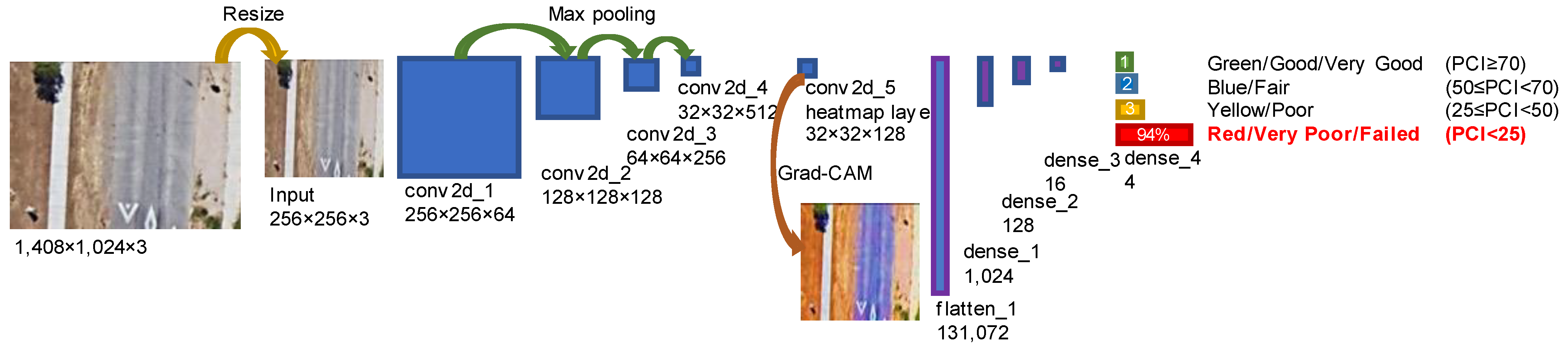
3.1. CNN Model for Classification and Visualization
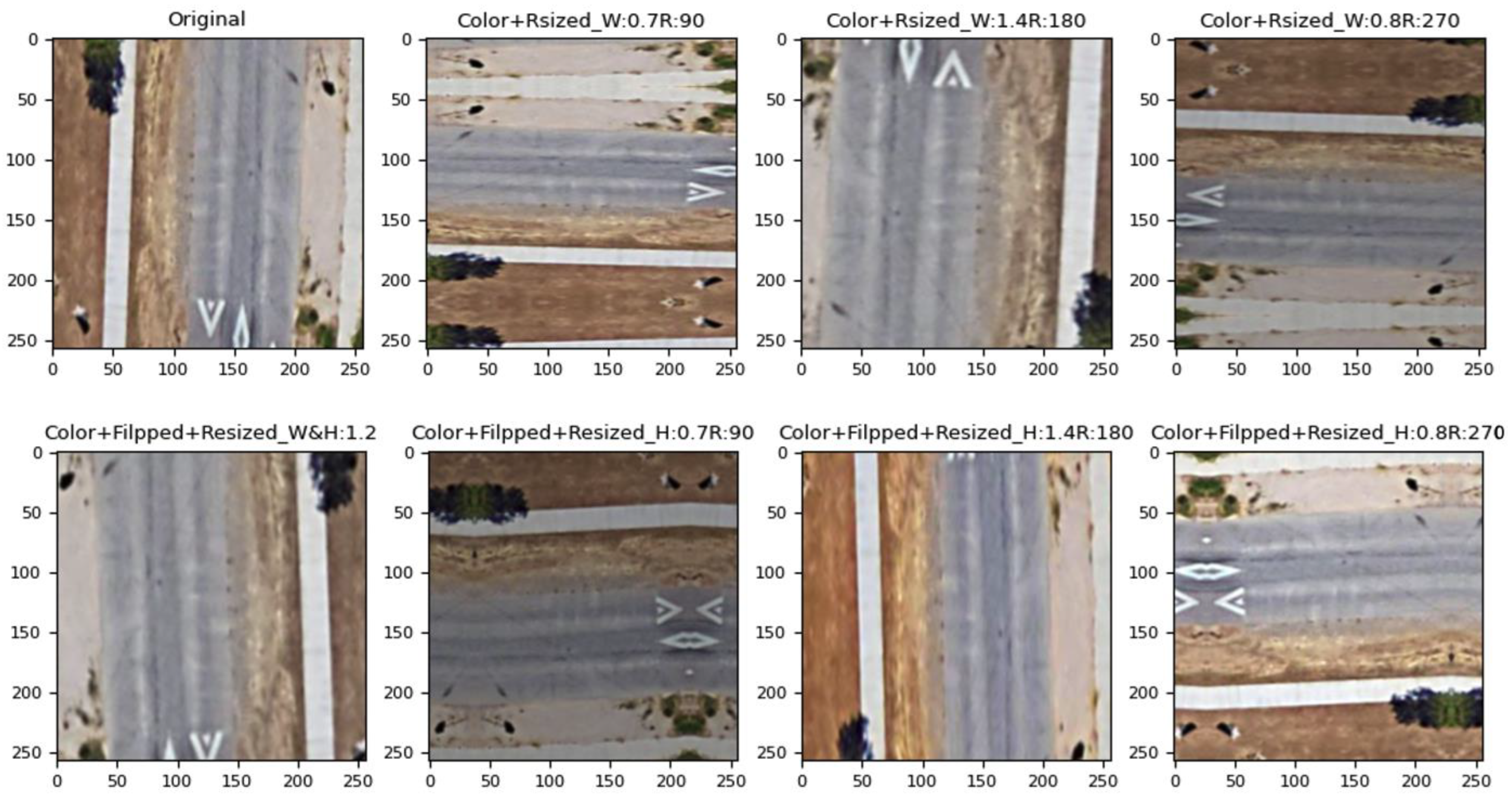
3.2. Data Augmentation
3.3. Evaluation Metrics
4. Experiments and Results
4.1. Dataset Preparation
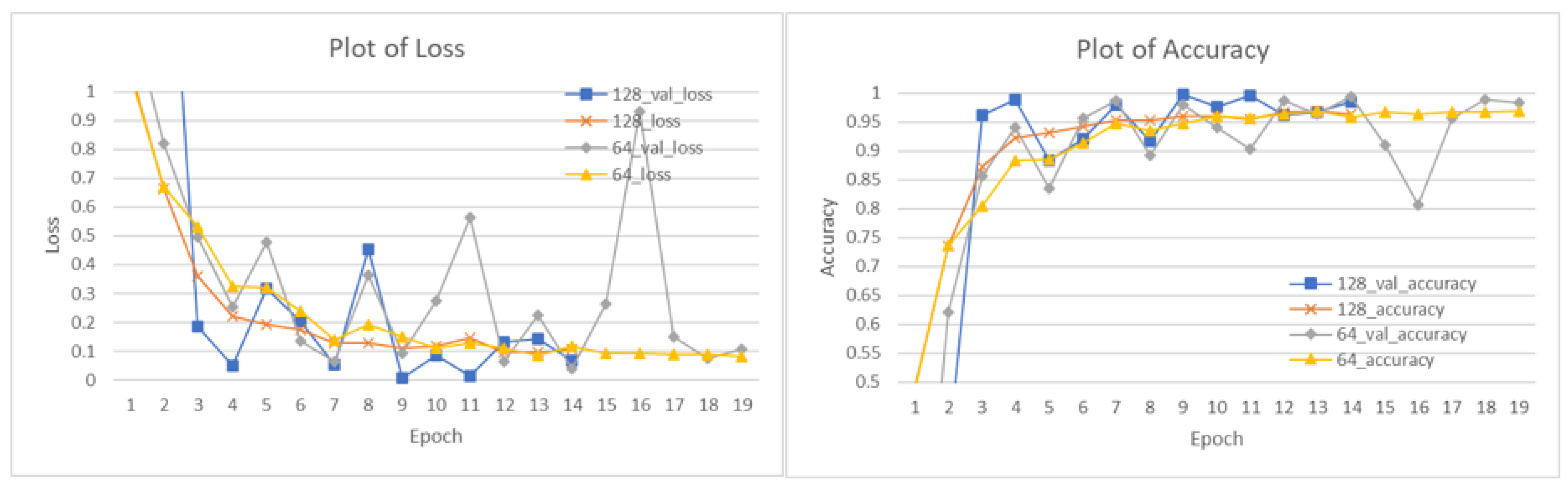
4.2. Model Training
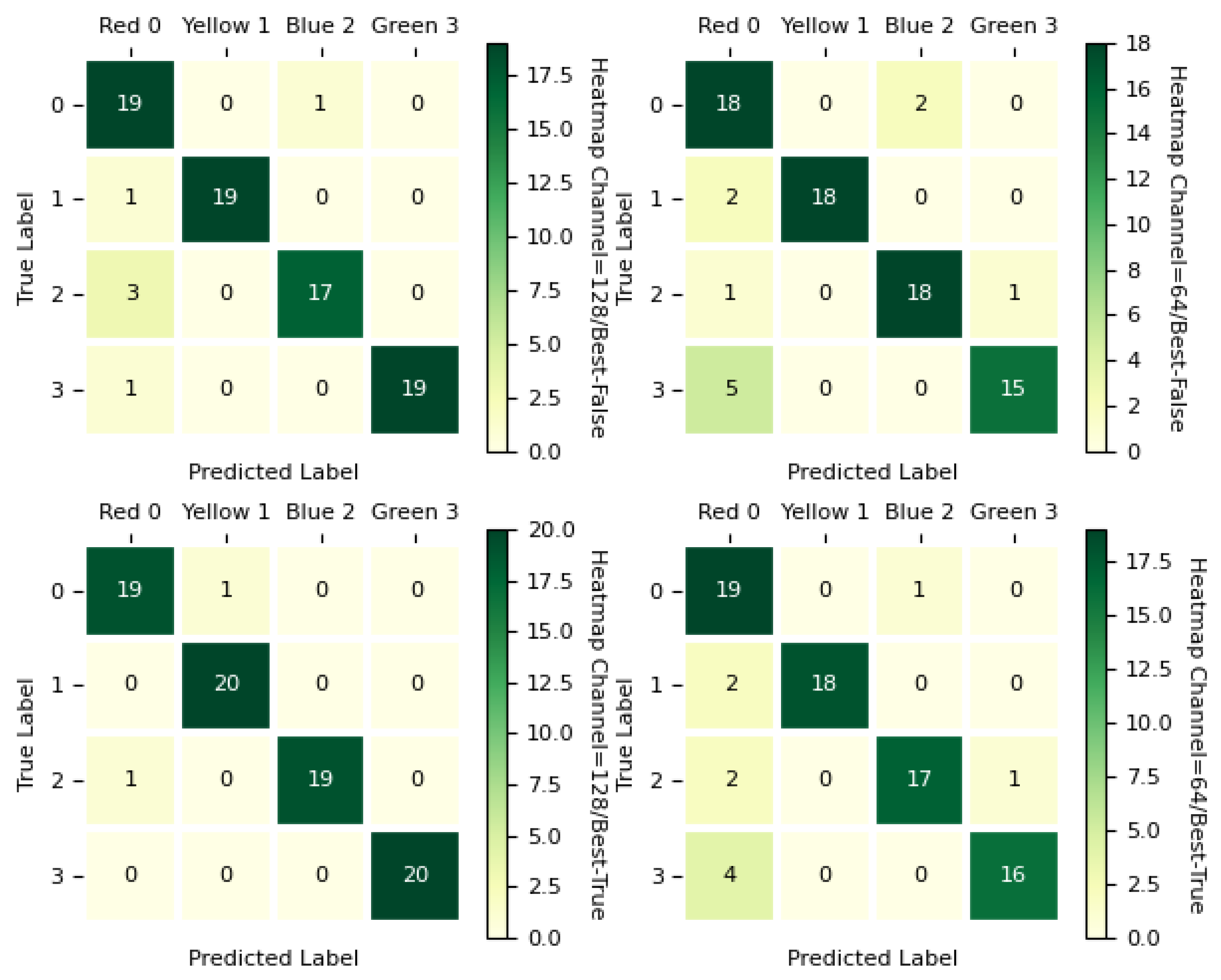
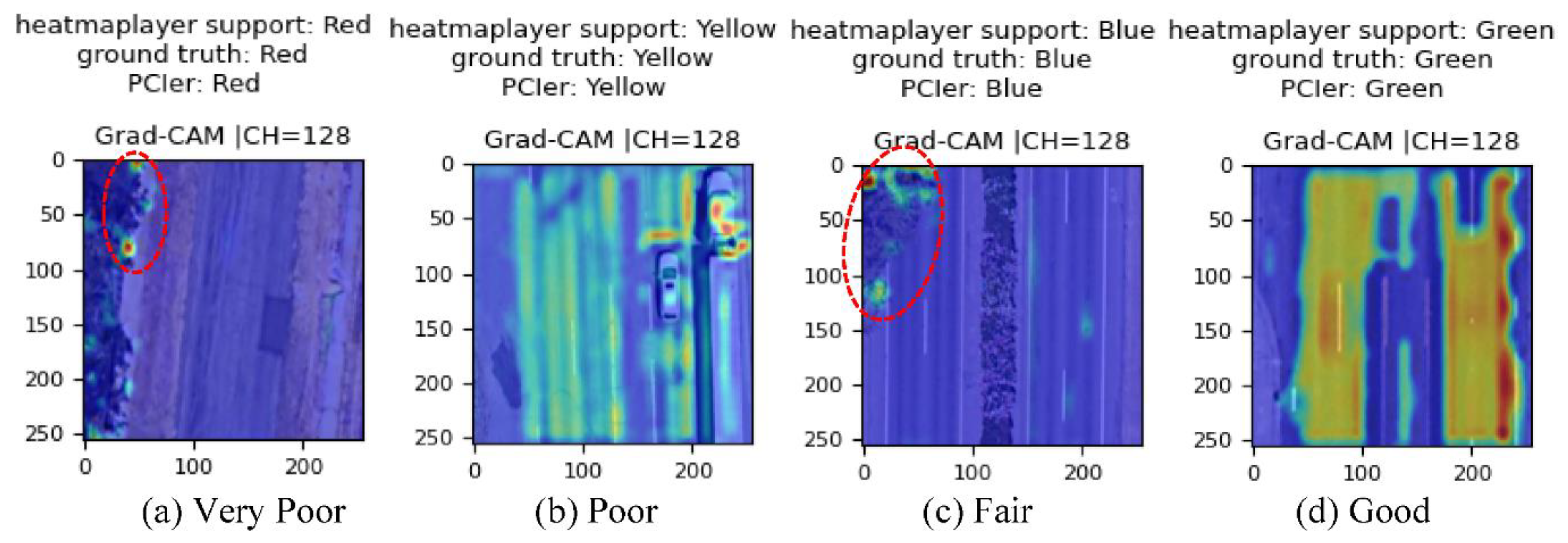
4.3. Model Testing
5. Discussion
5.1. Performance Comparison
5.2. Limitations
- (1)
- Collect more images for CNN model training to reduce the impact of non-street object obstruction on the classification results. In this approach, additional convolution layers (and channels) and dense layers may need to be added to the proposed CNN model for feature learning. Then, the complicated model might discard the vegetation zone.
- (2)
- Remove non-street (pavement) surfaces from the collected image. In this approach, the vegetation zone would be cropped, and only the street surface would show in the input images for the proposed CNN model.
5.3. Recommendation
6. Conclusions
Author Contributions
Funding
Data Availability Statement
Acknowledgments
Conflicts of Interest
References
- Texas Department of Transportation Pavement Manual. Available online: http://onlinemanuals.txdot.gov/txdotmanuals/pdm/index.htm (accessed on 14 January 2023).
- Fuentes, L.; Camargo, R.; Martínez-Arguelles, G.; Komba, J.J.; Naik, B.; Walubita, L.F. Pavement Serviceability Evaluation Using Whole Body Vibration Techniques: A Case Study for Urban Roads. Int. J. Pavement Eng. 2021, 22, 1238–1249. [Google Scholar] [CrossRef]
- Fuentes, L.; Taborda, K.; Hu, X.; Horak, E.; Bai, T.; Walubita, L.F. A Probabilistic Approach to Detect Structural Problems in Flexible Pavement Sections at Network Level Assessment. Int. J. Pavement Eng. 2022, 23, 1867–1880. [Google Scholar] [CrossRef]
- Matlack, G.R.; Horn, A.; Aldo, A.; Walubita, L.F.; Naik, B.; Khoury, I. Measuring Surface Texture of In-Service Asphalt Pavement: Evaluation of Two Proposed Hand-Portable Methods. Road Mater. Pavement Des. 2023, 24, 592–608. [Google Scholar] [CrossRef]
- ASTM D6433 2020; ASTM International Standard Practice for Roads and Parking Lots Pavement Condition Index Surveys. ASTM: West Conshohocken, PA, USA.
- Chambon, S.; Moliard, J.M. Automatic Road Pavement Assessment with Image Processing: Review and Comparison. Int. J. Geophys. 2011, 2011, 989354. [Google Scholar] [CrossRef]
- Ji, A.; Xue, X.; Wang, Y.; Luo, X.; Xue, W. An Integrated Approach to Automatic Pixel-Level Crack Detection and Quantification of Asphalt Pavement. Autom. Constr. 2020, 114, 103176. [Google Scholar] [CrossRef]
- Wang, W.; Wang, M.; Li, H.; Zhao, H.; Wang, K.; He, C.; Wang, J.; Zheng, S.; Chen, J. Pavement Crack Image Acquisition Methods and Crack Extraction Algorithms: A Review. J. Traffic Transp. Eng. 2019, 6, 535–556. [Google Scholar] [CrossRef]
- Kheradmandi, N.; Mehranfar, V. A Critical Review and Comparative Study on Image Segmentation-Based Techniques for Pavement Crack Detection. Constr. Build. Mater. 2022, 321, 126162. [Google Scholar] [CrossRef]
- Li, W.; Huyan, J.; Gao, R.; Hao, X.; Hu, Y.; Zhang, Y. Unsupervised Deep Learning for Road Crack Classification by Fusing Convolutional Neural Network and K_Means Clustering. J. Transp. Eng. Part B Pavements 2021, 147, 04021066. [Google Scholar] [CrossRef]
- Jiang, Y.; Han, S.; Bai, Y. Development of a Pavement Evaluation Tool Using Aerial Imagery and Deep Learning. J. Transp. Eng. Part B Pavements 2021, 147, 04021027. [Google Scholar] [CrossRef]
- Jiang, Y.; Bai, Y.; Han, S. Determining Ground Elevations Covered by Vegetation on Construction Sites Using Drone-Based Orthoimage and Convolutional Neural Network. J. Comput. Civ. Eng. 2020, 34, 04020049. [Google Scholar] [CrossRef]
- Zhang, C.; Nateghinia, E.; Miranda-Moreno, L.F.; Sun, L. Pavement Distress Detection Using Convolutional Neural Network (CNN): A Case Study in Montreal, Canada. Int. J. Transp. Sci. Technol. 2021, 11, 298–309. [Google Scholar] [CrossRef]
- Protopapadakis, E.; Voulodimos, A.; Doulamis, A.; Doulamis, N.; Stathaki, T. Automatic Crack Detection for Tunnel Inspection Using Deep Learning and Heuristic Image Post-Processing. Appl. Intell. 2019, 49, 2793–2806. [Google Scholar] [CrossRef]
- Maniat, M.; Camp, C.V.; Kashani, A.R. Deep Learning-Based Visual Crack Detection Using Google Street View Images. Neural Comput. Appl. 2021, 33, 14565–14582. [Google Scholar] [CrossRef]
- Zhou, S.; Song, W. Deep Learning-Based Roadway Crack Classification Using Laser-Scanned Range Images: A Comparative Study on Hyperparameter Selection. Autom. Constr. 2020, 114, 103171. [Google Scholar] [CrossRef]
- Ali, L.; Valappil, N.K.; Kareem, D.N.A.; John, M.J.; Al Jassmi, H. Pavement Crack Detection and Localization Using Convolutional Neural Networks (CNNs). In Proceedings of the 2019 International Conference on Digitization (ICD), Sharjah, United Arab Emirates, 18–19 November 2019; pp. 217–221. [Google Scholar]
- Fan, R.; Bocus, M.J.; Zhu, Y.; Jiao, J.; Wang, L.; Ma, F.; Cheng, S.; Liu, M. Road Crack Detection Using Deep Convolutional Neural Network and Adaptive Thresholding. In Proceedings of the 2019 IEEE Intelligent Vehicles Symposium (IV), Paris, France, 9–12 June 2019; Volume 2019, pp. 474–479. [Google Scholar]
- Jiang, Y. Remote Sensing and Neural Network-Driven Pavement Evaluation: A Review. In Proceedings of the The 12th International Conference on Construction in the 21st Century (CITC-12), Amman, Jordan, 16–19 May 2022; pp. 335–345. [Google Scholar]
- Dadrasjavan, F.; Zarrinpanjeh, N.; Ameri, A.; Engineering, G.; Branch, Q. Automatic Crack Detection of Road Pavement Based on Aerial UAV Imagery. Preprints 2019, 2019070009. [Google Scholar] [CrossRef]
- Edmondson, V.; Woodward, J.; Lim, M.; Kane, M.; Martin, J.; Shyha, I. Improved Non-Contact 3D Field and Processing Techniques to Achieve Macrotexture Characterisation of Pavements. Constr. Build. Mater. 2019, 227, 116693. [Google Scholar] [CrossRef]
- Roberts, R.; Inzerillo, L.; Di Mino, G. Exploiting Low-Cost 3D Imagery for the Purposes of Detecting and Analyzing Pavement Distresses. Infrastructures 2020, 5, 6. [Google Scholar] [CrossRef]
- Zhou, S.; Song, W. Robust Image-Based Surface Crack Detection Using Range Data. J. Comput. Civ. Eng. 2020, 34, 04019054. [Google Scholar] [CrossRef]
- Shi, Y.; Cui, L.; Qi, Z.; Meng, F.; Chen, Z. Automatic Road Crack Detection Using Random Structured Forests. IEEE Trans. Intell. Transp. Syst. 2016, 17, 3434–3445. [Google Scholar] [CrossRef]
- Tong, Z.; Yuan, D.; Gao, J.; Wei, Y.; Dou, H. Pavement-Distress Detection Using Ground-Penetrating Radar and Network in Networks. Constr. Build. Mater. 2020, 233, 117352. [Google Scholar] [CrossRef]
- Sukhobok, Y.A.; Verkhovtsev, L.R.; Ponomarchuk, Y.V. Automatic Evaluation of Pavement Thickness in GPR Data with Artificial Neural Networks. IOP Conf. Ser. Earth Environ. Sci. 2019, 272, 022202. [Google Scholar] [CrossRef]
- Jiang, Y.; Bai, Y. Estimation of Construction Site Elevations Using Drone-Based Orthoimagery and Deep Learning. J. Constr. Eng. Manag. 2020, 146, 04020086. [Google Scholar] [CrossRef]
- Selvaraju, R.R.; Cogswell, M.; Das, A.; Vedantam, R.; Parikh, D.; Batra, D. Grad-CAM: Visual Explanations from Deep Networks via Gradient-Based Localization. In Proceedings of the 2017 IEEE International Conference on Computer Vision (ICCV), Venice, Italy, 22–29 October 2017; Volume 128, pp. 618–626. [Google Scholar]
- Haeberli, P.; Voorhies, D. Image Processing By Interp and Extrapolation. Available online: http://www.graficaobscura.com/interp/index.html (accessed on 28 July 2021).
- Moore, R.; Montanez, J.; Smith, G.; Saenz, R. Pavement Condition Report. Available online: https://www.cityofsacramento.org/-/media/Corporate/Files/Public-Works/Maintenance-Services/Sacramento-2020-Pavement-Update---FINAL-3-25-20.pdf?la=en (accessed on 5 April 2022).
- Jiang, Y. PCIer—Pavement Condition Index Estimation. Available online: https://www.yuhanjiang.com/research/IM/PA/PCI (accessed on 15 January 2023).
- Zhang, A.; Wang, K.C.P.; Fei, Y.; Liu, Y.; Chen, C.; Yang, G.; Li, J.Q.; Yang, E.; Qiu, S. Automated Pixel-Level Pavement Crack Detection on 3D Asphalt Surfaces with a Recurrent Neural Network. Comput. Civ. Infrastruct. Eng. 2019, 34, 213–229. [Google Scholar] [CrossRef]


| Block | Layer | Filter and Size | Stride | Padding | Activation | Output Shape |
|---|---|---|---|---|---|---|
| Input | - | - | - | - | - | (256, 256, 3) |
| Feature learning | conv2d_1 | 64, 3, 3 | 1 | Same | ReLU | (256, 256, 64) |
| max_pooling2d_1 | 2, 2 | 2 | - | - | (128, 128, 64) | |
| conv2d_2 | 128, 3, 3 | 1 | Same | ReLU | (128, 128, 128) | |
| max_pooling2d_2 | 2, 2 | 2 | - | - | (64, 64, 128) | |
| conv2d_3 | 256, 3, 3 | 1 | Same | ReLU | (64, 64, 256) | |
| max_pooling2d_3 | 2, 2 | 2 | - | - | (32, 32, 256) | |
| conv2d_4 | 512, 3, 3 | 1 | Same | ReLU | (32, 32, 512) | |
| heatmap_layer (conv2d_5) | 128, 1, 1 or 64, 1, 1 | 1 | Same | ReLU | (32, 32, 128) or (32, 32, 64) | |
| Classification | flatten_1 | - | - | - | - | 131,072 or 65,536 |
| dropout_1 | 0.5 | - | - | - | 131,072 or 65,536 | |
| dense_1 | 1024 | - | - | ReLU | 1024 | |
| dropout_2 | 0.5 | - | - | - | 1024 | |
| dense_2 | 128 | - | - | ReLU | 128 | |
| dropout_3 | 0.5 | - | - | - | 128 | |
| dense_3 | 16 | - | - | ReLU | 16 | |
| dropout_4 | 0.5 | - | - | - | 16 | |
| Output | dense_4 | 4 | - | - | SoftMax | 4 |
| - | - | - | - | Argmax | 1 (Prediction) |
| Street Name | PCI Grade | Collected Image | Training | Testing | Original Image Size | Image Size |
|---|---|---|---|---|---|---|
| College Town Dr | Very Poor (PCI < 25) | 55 | 45 | 10 | 1408 × 1024-pixel | 256 × 256-pixel |
| Main Avenue | Very Poor (PCI < 25) | 45 | 35 | 10 | 1408 × 1024-pixel | 256 × 256-pixel |
| Florin Perkins Rd | Poor (25 ≤ PCI < 50) | 100 | 80 | 20 | 1408 × 1024-pixel | 256 × 256-pixel |
| Freeport Blvd | Fair (50 ≤ PCI < 70) | 100 | 80 | 20 | 1408 × 1024-pixel | 256 × 256-pixel |
| Power Inn Rd | Good (PCI ≥ 70) | 100 | 80 | 20 | 1408 × 1024-pixel | 256 × 256-pixel |
| PCI Grade | 128-Channel Final Model | 64-Channel Final Model | 128-Channel Best Model | 64-Channel Best Model | Support | ||||||||
|---|---|---|---|---|---|---|---|---|---|---|---|---|---|
| Precision | Recall | F1-Score | Precision | Recall | F1-Score | Precision | Recall | F1-Score | Precision | Recall | F1-Score | ||
| Very Poor | 0.79 | 0.95 | 0.86 | 0.69 | 0.90 | 0.78 | 0.95 | 0.95 | 0.95 | 0.70 | 0.95 | 0.81 | 20 |
| Poor | 1.00 | 0.95 | 0.97 | 1.00 | 0.90 | 0.95 | 0.95 | 1.00 | 0.98 | 1.00 | 0.90 | 0.95 | 20 |
| Fair | 0.94 | 0.85 | 0.89 | 0.90 | 0.90 | 0.90 | 1.00 | 0.95 | 0.97 | 0.94 | 0.85 | 0.89 | 20 |
| Good | 1.00 | 0.95 | 0.97 | 0.94 | 0.75 | 0.83 | 1.00 | 1.00 | 1.00 | 0.94 | 0.80 | 0.86 | 20 |
| accuracy | 0.93 | 0.86 | 0.97 | 0.88 | 80 | ||||||||
| macro avg | 0.93 | 0.93 | 0.93 | 0.88 | 0.86 | 0.87 | 0.98 | 0.97 | 0.97 | 0.90 | 0.88 | 0.88 | 80 |
| weighted avg | 0.93 | 0.93 | 0.93 | 0.88 | 0.86 | 0.87 | 0.98 | 0.97 | 0.97 | 0.90 | 0.88 | 0.88 | 80 |
Disclaimer/Publisher’s Note: The statements, opinions and data contained in all publications are solely those of the individual author(s) and contributor(s) and not of MDPI and/or the editor(s). MDPI and/or the editor(s) disclaim responsibility for any injury to people or property resulting from any ideas, methods, instructions or products referred to in the content. |
© 2023 by the authors. Licensee MDPI, Basel, Switzerland. This article is an open access article distributed under the terms and conditions of the Creative Commons Attribution (CC BY) license (https://creativecommons.org/licenses/by/4.0/).
Share and Cite
Han, S.; Chung, I.-H.; Jiang, Y.; Uwakweh, B. PCIer: Pavement Condition Evaluation Using Aerial Imagery and Deep Learning. Geographies 2023, 3, 132-142. https://doi.org/10.3390/geographies3010008
Han S, Chung I-H, Jiang Y, Uwakweh B. PCIer: Pavement Condition Evaluation Using Aerial Imagery and Deep Learning. Geographies. 2023; 3(1):132-142. https://doi.org/10.3390/geographies3010008
Chicago/Turabian StyleHan, Sisi, In-Hun Chung, Yuhan Jiang, and Benjamin Uwakweh. 2023. "PCIer: Pavement Condition Evaluation Using Aerial Imagery and Deep Learning" Geographies 3, no. 1: 132-142. https://doi.org/10.3390/geographies3010008
APA StyleHan, S., Chung, I.-H., Jiang, Y., & Uwakweh, B. (2023). PCIer: Pavement Condition Evaluation Using Aerial Imagery and Deep Learning. Geographies, 3(1), 132-142. https://doi.org/10.3390/geographies3010008