Death as Rising Entropy: A Theory of Everything for Postmortem Interval Estimation

Abstract

Determining the postmortem interval remains one of the most persistent and fragmented challenges in forensic science. Conventional approaches—thermal, biochemical, molecular, or entomological—capture only isolated fragments of a single physical reality: the irreversible drift of a once-living system toward equilibrium. This Perspective proposes a unifying paradigm in which death is understood as a progressive rise in entropy, encompassing the loss of biological order across thermal, chemical, structural, and ecological domains. Each measurable postmortem variable—temperature decay, metabolite diffusion, macromolecular breakdown, tissue disorganization, and microbial succession—represents a distinct expression of the same universal law. Within this framework, entropy becomes a dimensionless index of disorder that can be normalized and compared across scales, transforming scattered empirical data into a coherent continuum. A Bayesian formulation further integrates these entropic signals according to their temporal reliability, yielding a probabilistic, multidomain equation for PMI estimation. By merging thermodynamics, information theory, and biology, the concept of death as rising entropy offers a comprehensive physical description of the postmortem process and a theoretical foundation for future computational, imaging, and metabolomic models in forensic time analysis.

1. Introduction

The estimation of the postmortem interval (PMI) remains one of the most enduring and consequential challenges in forensic practice. Its determination is central to event reconstruction, alibi evaluation, and identification in mass-fatality contexts. Despite more than a century of work, no single method has achieved universal reliability. Classic signs—body cooling, rigor mortis, and livor mortis—remain in routine use, yet their reliability is limited, and their interpretive window is narrow [1,2]. Contemporary reviews confirm that decomposition depends both on external factors (temperature, humidity, insect activity) and on intrinsic characteristics such as body mass, pathology, and microbiome composition. This makes PMI estimation inherently complex and context-dependent [3,4]. Attempts to refine early postmortem estimations have largely focused on temperature-based models, with the Henssge nomogram representing the most structured effort to formalize algor mortis using parameters such as body weight and ambient temperature. While methodologically influential, its practical performance is highly dependent on stable environmental conditions that are seldom present in casework. The frequently cited 36.8% concordance with the actual time of death originates from a single study conducted under specific experimental conditions, and other investigations have reported different levels of accuracy. This figure should, therefore, be viewed as an example of context-dependent variability, underscoring the difficulty of applying single-parameter thermal models in heterogeneous real-world scenarios [5]. Subsequent exchanges between investigators and critics emphasized that the model was derived from limited case material and lacks the external validation required for forensic reliability [5,6]. Even under ideal conditions, confounding factors such as clothing, body surface area, and body mass index substantially reduce precision [7]. Other classical indicators, such as rigor and livor mortis, have proven equally inconsistent. Rigor mortis, once considered a predictable sequence of stiffening and relaxation, is affected by temperature, exertion, and pathological status, and may even reappear outside its canonical window [6]. Livor mortis is assessed qualitatively and shows high inter-observer variability, with progression strongly dependent on ambient conditions and body position [4]. Supravital reactions—initially thought to provide precise temporal markers—are short-lived, variable, and resistant to standardization [8]. To extend applicability beyond the early hours after death, anthropological models such as the Total Body Score (TBS) combined with Accumulated Degree-Days (ADD) link decomposition with environmental energy input. These systems are attractive for their structured scoring and adaptability to fieldwork [9], but results vary across climates and ecological zones, limiting claims of universality. Field studies in South Africa demonstrated significant inaccuracies when ADD models were applied outside temperate regions [10], and although improved mathematical formulations have been proposed [11], systematic reviews and meta-analyses confirm that prediction intervals remain too broad for forensic or judicial certainty [9,12]. Parallel efforts have explored biochemical and imaging-based strategies. Vitreous humor analysis, once promising for its relative stability, has yielded variable results depending on storage conditions and cause of death. Studies on DNA and RNA degradation suggest temporal signatures, but their rates are highly dependent on temperature and tissue type [4]. Proteomic markers such as creatine kinase or GAPDH have been investigated, yet findings are inconsistent and often based on small sample sets. Emerging imaging modalities—including postmortem computed tomography, magnetic resonance imaging, and optical coherence tomography—have provided proof-of-concept evidence that structural changes may carry chronological information [13]. However, these remain fragmented innovations: each method illuminates only a narrow segment of the postmortem timeline, and none has matured into a universally accepted protocol. Analyses of Dutch case law reveal that PMI methods, though frequently invoked, often fail to satisfy these requirements [14]. The lack of standardized protocols, the sensitivity to uncontrollable variables, and the reliance on subjective interpretation diminish their credibility in adversarial contexts. Scholarly reviews echo these concerns, underscoring that dependence on narrow or poorly validated models risks overconfidence and misrepresentation in judicial proceedings [4,13]. Taken together, these limitations illustrate a central paradox of forensic chronobiology: the demand for accuracy is greatest where uncertainty is most profound. Temperature-based models, stiffness and lividity, decomposition scores, biochemical assays, and imaging methods each provide valuable fragments of information, yet they do not offer a comprehensive or fully reproducible solution. Their limitations in generalizability, reproducibility, and legal robustness underscore the need for a unified physical framework capable of integrating heterogeneous postmortem signals into a coherent temporal structure. The present work proposes a unifying physical framework in which these heterogeneous phenomena are expressed through a single, dimensionless variable: entropy. By translating the results of virtually all established PMI estimation methods into entropic terms, we show that each method describes a different projection of the same irreversible process—the progressive loss of order and the drift toward equilibrium. This empirical translatability gives the model its “theory of everything” characteristic: not by explaining all things, but by encompassing the totality of measurable postmortem changes within one quantitative law. Once normalized, this approach allows a direct comparison between domains and time scales, potentially enabling the same physical quantity to describe deaths separated by hours or by several days. In this sense, the model does not replace traditional techniques but integrates them within a single thermodynamic continuum, transforming PMI estimation from an empirical extrapolation into a physics-based inference problem.

Why “Theory of Everything”

The expression “Theory of Everything” is used here not in its cosmological sense, but as a shorthand for empirical completeness. In forensic science, the fragmentation of methods—thermal, biochemical, structural, and microbial—has long prevented a unified description of postmortem change. Each approach captures a different projection of the same irreversible process, yet their outputs remain confined to incompatible scales.

By translating the results of virtually all established PMI estimation techniques into a single quantitative variable—entropy—this framework achieves an operational form of totality: it allows every measurable manifestation of death to be expressed along the same physical continuum. The “everything”, therefore, refers to the scope of integration, not to metaphysical ambition. The model does not claim to explain all processes of decay, but to encompass the totality of reproducible observations through a single mathematical law.

Once normalized, entropy becomes a shared metric connecting different domains, body conditions, and temporal scales. It potentially enables the same physical quantity to describe both an individual dead for one hour and another dead for several days. In this sense, the theory aspires not to universality in the philosophical sense, but to interoperability in the scientific one—a bridge among all valid quantitative descriptions of dying.

2. Death as Rising Entropy

The search for a single law capable of encompassing all postmortem transformations naturally leads to the thermodynamic principle of entropy.

Entropy is not an abstract or metaphysical idea; it is a measurable property describing how a system evolves from order to disorder. Entropy (S) quantifies the number of microstates accessible to a system at a given energy level and thus its degree of disorder, according to Boltzmann’s definition:

S = k ln W

where k is the Boltzmann constant, and W is the number of possible microstates. While Boltzmann entropy quantifies physical microstates, Shannon entropy describes uncertainty in state distributions; both share the same mathematical form, linking energy dispersion to informational disorder.

Every living organism represents an improbable pocket of order maintained by continuous energy flow, molecular coordination, and information control. When this regulation ceases, gradients flatten, correlations vanish, and entropy rises.

In thermodynamics, entropy quantifies the dispersion of energy—the degree to which heat or chemical potential becomes unavailable for work, a concept first formalized by Rudolf Clausius in 1864 and later extended to complex systems [15,16]. Living cells postpone this process through metabolism, exporting entropy to the environment to preserve internal structure [17]. When metabolism stops, temperature and electrochemical gradients collapse, ATP breaks down, and ions diffuse freely. These macroscopic and microscopic transitions—cooling, ionic leakage, and rigor mortis—represent measurable manifestations of rising thermodynamic entropy.

In information theory, entropy assumes a complementary meaning. Claude Shannon (1948) defined informational entropy as the average uncertainty of a system, formalized as H = −Σ p log p, expressing the number of possible states a system can occupy: the greater the unpredictability, the higher the entropy [18]. Building upon Shannon’s framework, Machado and Lopes extended this concept to human mortality, demonstrating that the uncertainty of death itself can be described through Shannon and cumulative residual entropies [19]. Their model shows that as survival probability declines, life progressively resolves its own unpredictability—an elegant bridge between informational and biological entropy.

In living organisms, predictable patterns—regular heartbeats, stable gene expression, and organized tissue morphology—reflect low informational entropy. After death, these regularities vanish: electrical rhythms flatten, macromolecules fragment, and tissue architecture disintegrates. The dissolution of predictable structure transforms biological information into statistical noise, the informational counterpart of thermodynamic decay. Recent advances in systems and computational biology have revealed that life itself can be described as a continuous exchange of information between molecular “senders” and “receivers” [20]. Signal-transduction networks, feedback loops, and metabolic circuits transmit biochemical messages with finite “channel capacity.” As long as this internal communication remains intact, uncertainty remains low. When circulation stops, these informational channels fail, mutual information collapses, and randomness expands. Informational entropy thus rises in parallel with thermodynamic entropy, linking the physical and computational dimensions of biological order. From a theoretical perspective, biological systems persist by managing entropy flow: they maintain low internal entropy through metabolic coupling that exports disorder outward [17]. Gladyshev described this through temporal hierarchies, where higher biological levels (organs, tissues) decay first after systemic regulation ceases, releasing lower levels (cells, molecules) to equilibrate independently [21]. The loss of this hierarchical coordination—rather than a single catastrophic event—marks the true beginning of death. At the statistical level, Aristov et al. demonstrated that cooperative correlations between subsystems minimize total entropy in living matter; when these correlations vanish, entropy rises abruptly [22]. This observation captures Schrödinger’s notion of “feeding on negentropy” in measurable physical terms. Bailly and Longo introduced the concept of “anti-entropy” to describe biological organization as an active, self-regenerating order distinct from structural regularity; death thus represents the disappearance of anti-entropy—the irreversible loss of self-repair and self-prediction [23]. Information-theoretic analyses reinforce this view. As emphasized by Chanda et al., biological systems are inherently noisy across molecular hierarchies—from gene expression to metabolomic networks—and entropy provides a unifying metric for quantifying that noise [24]. Summers further argued that organisms survive by dynamically regulating uncertainty, reducing surprise through feedback, consistent with Friston’s free-energy principle [25,26]. When this regulatory loop fails, both thermodynamic and informational entropy accelerate in tandem. Natural systems, as shown by Martyushev and Seleznev, evolve to maximize entropy production until equilibrium is reached [27]. Mitrokhin emphasized that thermodynamic and informational entropy coexist in biology and unravel simultaneously at death. The dying organism therefore follows a predictable entropic trajectory: residual metabolism briefly resists disorder, but once energy reserves are exhausted, gradients collapse, and randomness dominates. Entropy, in this sense, is not merely an endpoint—it represents the slope of dying itself [28].

Forensic observation fits seamlessly into this framework. Every postmortem change—body cooling, hypostasis, rigor, cellular autolysis, and DNA fragmentation—represents a stage in the rise in entropy across biological scales. These processes can be quantified in physical units (J/K, bits) or statistical indices, linking molecular and macroscopic phenomena under one law. Entropy transforms the descriptive language of decomposition into a measurable continuum of disorder. Brooks and Wiley famously described life as a temporary negation of entropy, a fleeting improbability maintained through continuous work. When that work ceases, the improbability collapses [29]. Thus, death as rising entropy is not metaphorical but physical: a trajectory from low to maximal entropy encompassing all observable signs of biological cessation. By framing the postmortem interval as a quantifiable entropic ascent, forensic science gains a unifying principle that bridges thermodynamics, information theory, and biology, turning the decay of order into a measurable chronometer of death [30].

2.1. Entropy as Progressive Loss of Biological Order

The transition from metabolic order to thermodynamic equilibrium unfolds as a continuous loss of organization across physical and informational hierarchies.

From a physical perspective, death marks the interruption of the metabolic flow that kept a living organism far from thermodynamic equilibrium. When circulation and respiration cease, the continuous exchange of energy and information that sustains cellular order comes to an end, and all gradients—thermal, chemical, and electrical—begin to dissipate spontaneously. This transition represents a progressive increase in entropy, measurable as both the loss of organization and the equalization of potential differences within the system. In the minutes following cardiac arrest, residual metabolic reactions persist transiently. Oxygen tension declines, ATP synthesis stops, and ionic pumps fail, leading to passive diffusion of ions across membranes. pH decreases, mitochondrial potential collapses, and body temperature begins to equilibrate with the environment. These processes correspond to an early thermodynamic drift: the energy used to preserve structure and function becomes uniformly distributed, increasing systemic disorder. At the molecular level, enzymatic control deteriorates and macromolecules lose conformational stability. Proteins unfold, nucleic acids undergo hydrolysis, and the cytoskeleton disassembles. The selective compartmentalization of the living state gives way to unrestricted diffusion, allowing metabolites, ions, and water to move according to purely physical laws. Each of these transitions contributes to the rise in entropy, quantifiable either as energy dispersion (ΔS = Q/T) or as loss of informational order (Shannon entropy). As time progresses, the breakdown of regulatory hierarchies propagates to tissues and organs. Mechanical stiffness, osmotic balance, and optical properties—such as corneal transparency—change predictably as entropy increases. Structural coherence decays into homogeneity, and the gradients that defined the living architecture vanish. The organism approaches thermal and chemical equilibrium with its surroundings—the maximal entropic state for the system. This continuum, rather than a discrete event, constitutes the physical basis for PMI estimation. Every measurable postmortem change—temperature decrease, biochemical drift, molecular degradation, or morphological alteration—represents a specific domain of the same entropic process. Quantifying this progression through diverse observable variables allows the PMI to be expressed as a function of entropy rather than as a purely empirical timeframe [30].

2.2. Why Entropy Provides an Integrative Framework for PMI Estimation

Entropy is proposed not as an additional forensic parameter, but as a unifying physical quantity capable of translating heterogeneous postmortem changes onto a common dimensionless scale. Several properties justify its use as an integrative variable. First, entropy rises monotonically after death: once metabolic energy supply ceases, every biological system moves irreversibly toward thermodynamic equilibrium, ensuring a consistent directionality of the entropic signal across domains. Second, entropy is additive for independent components, allowing thermal, biochemical, microstructural, and ecological contributions to be combined on the same informational basis without violating physical coherence. Third, entropy is scale-invariant: because it is expressed in dimensionless form, measurements obtained at microscopic, macroscopic, biochemical, or ecological levels can be normalized to a 0–1 interval and compared directly. Fourth, entropy preserves information, capturing the progressive loss of biological order even when individual biomarkers exhibit domain-specific noise. Finally, entropy is mathematically invertible under simple functional forms (exponential or logistic), allowing entropic values to be translated back into temporal estimates with analytically tractable uncertainty. Taken together, these features—monotonicity, additivity, scale-invariance, information preservation, and invertibility—justify entropy as the most appropriate unifying variable for describing heterogeneous postmortem phenomena within a single framework.

2.3. Translating Empirical Measurements into an Entropic Scale

Once entropy is identified as the common physical language of postmortem change, the practical question becomes how standard forensic measurements can be expressed in entropic terms. This does not require reconstructing the full thermodynamic history of the body but simply locating each variable along its postmortem trajectory and rescaling it onto a 0–1 dimensionless continuum. Temperature offers the clearest example. As the corpse cools, the gradient between body temperature and the environment progressively decreases; expressing the residual gradient as a fraction of the initial one yields a monotonic thermal-entropy index. The same approach applies to biochemical variables. Electrolytes, metabolites, and macromolecular products can be positioned between their physiological baselines and their late postmortem plateaus, transforming biochemical drift into a normalized indicator of the loss of internal regulation. Structural and imaging-derived information can be handled similarly. The progressive disruption of tissue organization—reflected in changes in corneal transparency, optical scattering, or microscopic texture—can be quantified with metrics such as Shannon entropy and normalized to the same 0–1 scale. Across these examples, the principle is identical: each postmortem measurement reflects a portion of the system’s loss of order, and this progression can be expressed as a dimensionless, monotonic indicator of postmortem evolution. In this manner, thermal, biochemical, and structural data become directly comparable along a single entropic trajectory.

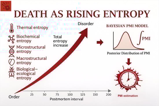
3. Entropic Domains of Postmortem Transformation

The concept of death as rising entropy becomes fully tangible only when examined through the hierarchy of transformations that unfold from the moment biological order begins to fail. Entropy does not increase within a single domain but propagates through successive layers of organization, each governed by its own physical and biochemical principles.

Immediately after cardiac arrest, the body behaves as a closed thermodynamic system, still attempting to maintain internal equilibrium. During this phase, entropy rises internally across four interconnected domains—thermal, biochemical, microstructural, and macrostructural—each marking a measurable step in the collapse of organization and predictability. Heat dissipates, chemical gradients flatten, cellular architecture disintegrates, and tissue coherence vanishes.

At a later stage, the system ceases to be closed. Its boundaries dissolve, and the corpse merges with the surrounding environment. This marks the onset of a fifth, biological–ecological domain, in which external biological agents—microbes, insects, and decomposers—become active participants in entropy production. The once self-contained system opens to exchanges of matter, energy, and information with the ecosystem.

Together, these five domains describe a continuous thermodynamic trajectory in which the postmortem system evolves irreversibly toward equilibrium. The first four belong to the physics of a closed biological system (internal disorganization), while the fifth marks the transition to an open system where decomposition becomes ecological.

The five entropic domains can be summarized as follows:

(1)

Thermal entropy—dissipation of residual metabolic heat;

(2)

Biochemical entropy—diffusion and equilibration of metabolites and ions;

(3)

Microstructural entropy—molecular and subcellular degradation (DNA, RNA, proteins);

(4)

Macrostructural entropy—loss of tissue and organ coherence observable through imaging;

(5)

Biological–ecological entropy—incorporation of the body into the environmental energy flow.

3.1. Methods: Deriving and Comparing Entropy Across Domains

To render the concept of rising entropy operational, each domain of the postmortem process must be expressed as a measurable function of disorder. Although the nature of the variables differs across physical, chemical, and structural scales, the same mathematical principle applies in that entropy increases as gradients vanish and variability becomes maximal.

For the purposes of this framework, entropy in each domain (S_i) is defined as a dimensionless index ranging from 0 (complete order) to 1 (maximum disorder).

In this manuscript, ‘microstructural entropy’ refers to molecular and subcellular degradation processes (DNA/RNA fragmentation, protein denaturation, peptide breakdown), i.e., changes occurring at the microscopic level. ‘Macrostructural entropy,’ instead, denotes tissue- and organ-level disorganization assessable through imaging or gross morphology. This terminology is used consistently across all five entropic domains.

(1)

Thermal entropy (S₁)—reduction in temperature differentials between body and environment, normalized by the initial gradient (ΔT₀).

(2)

Biochemical entropy (S₂)—equalization of metabolite and ion concentrations, e.g., vitreous potassium or lactate.

(3)

Microstructural entropy (S₃)—molecular disorganization quantified from fragment-size or conformational distributions.

(4)

Macrostructural entropy (S₄)—tissue-level disintegration measurable by radiomic or texture-based entropy.

(5)

Biological–ecological entropy (S₅)—microbial diversification and ecological succession describing the body’s integration into environmental energy flow.

Each S_i(t) increases monotonically with postmortem time t. Mapping all indices onto a common 0–1 scale allows the construction of a composite trajectory:

$${\mathit{S}}_{\mathit{t}\mathit{o}\mathit{t}\mathit{a}\mathit{l}\left(\mathit{t}\right)}=\sum _{\mathbf{i}}{\mathit{w}}_{\mathbf{i}\left(\mathit{t}\right){\mathit{S}}_{\mathbf{i}\left(\mathbf{t}\right)}}$$

where the weights w_i(t) represent the relative reliability of each domain as a function of time. In early postmortem phases, thermal and biochemical entropy dominate; in later intervals, structural and ecological components become more informative.

The calibration of w_i(t) can, in principle, be achieved empirically by evaluating the predictive accuracy of each domain within specific postmortem intervals. However, in this theoretical formulation, the weights remain conceptual placeholders for empirical confidence, representing the dynamic contribution of each domain to the total entropic rise. This framework provides a universal procedure for converting any measurable postmortem variable into an entropic expression comparable across scales. For practical implementation, each entropic domain can be calibrated using simple reference conditions. Thermal entropy aligns with controlled cooling curves at fixed ambient temperatures; biochemical and macromolecular entropy use baseline and end-point values obtained under defined storage conditions; structural entropy is normalized using imaging phantoms with stable optical properties; and microbial–ecological entropy is calibrated through standardized sequencing pipelines. These minimal reference conditions establish the calibration bounds (E₀, Emax) and rate constants (k) required for reproducible entropic indices across studies.

3.2. Thermal Domain: Dissipation of Residual Heat

The first and most fundamental manifestation of postmortem entropy is the dissipation of residual heat. With the cessation of metabolism, internal temperature gradients vanish as the organism moves toward equilibrium with its surroundings. According to the second law of thermodynamics, this spontaneous heat transfer corresponds to an entropy increase:

$$\mathit{\Delta }\mathit{s}=\mathit{C}\mathit{ln}\left({\displaystyle \frac{{\mathit{T}}_{\mathit{f}}}{{\mathit{T}}_{\mathbf{0}}}}\right)$$

where T₀ and T_f denote the core temperature at death and at time t, respectively. Body cooling follows an exponential decay consistent with Newton’s law and its forensic adaptation by Henssge [31,32,33]; simplified analytical models [34] and validation studies [35] show monotonic decay with rate constant k_t dependent on body mass, clothing, and ambient temperature. The normalized thermal entropy is defined as follows:

$${\mathit{E}}_{\mathit{t}\mathit{h}\mathit{e}\mathit{r}\mathit{m}\left(\mathit{t}\right)}=\mathbf{1}-{\mathit{e}}^{-\mathit{k}\mathit{t}},$$

rising from 0 (complete order) to 1 (thermal equilibrium).

The entropic expression of the PMI is obtained by inversion of the same relationship:

$$\mathit{P}\mathit{M}\mathit{I}=-{\displaystyle \frac{\mathbf{1}}{\mathit{k}}}\mathit{l}\mathit{n}\left(\mathbf{1}-{\mathit{E}}_{\mathit{t}\mathit{h}\mathit{e}\mathit{r}\mathit{m}}\right)$$

Under constant conditions, k_t typically ranges between 0.08 and 0.15 h⁻¹, producing an entropy rise that stabilizes within the first 24 h. In this formulation, k_t (h⁻¹) represents the thermal rate constant governing the exponential cooling process.

As shown in Figure 1A, the thermal entropy curves are adapted from the experimental dataset of Heinrich [35], who validated the Henssge model [1] using human cadavers stored at different ambient temperatures (≈10 °C and ≈20 °C). In that dataset, the measured temperature decay remains consistent with Newton’s exponential law, but when expressed as normalized entropy, it appears quasi-sigmoidal due to sampling resolution and limited temporal coverage, although the underlying physical model remains purely exponential. Entropy increases rapidly after death and gradually approaches equilibrium, with faster progression and higher asymptotic values at higher ambient temperatures, reflecting the modulatory effect of environmental heat exchange.

This thermal component represents the earliest and most deterministic contributor to the global entropic drift of the corpse. Its reproducibility and simplicity make it an ideal reference for normalizing the subsequent domains of postmortem entropy.

3.3. Biochemical Domain: Collapse of Metabolic Equilibrium

The biochemical domain captures the molecular loss of order that follows circulatory arrest.

Residual ATP and phosphocreatine transiently sustain ion pumps; as these energy reserves are depleted, sodium–potassium gradients fail, metabolites diffuse, lactate and hypoxanthine accumulate, and pH decreases.

These transitions reflect the spontaneous equalization of chemical potentials and the monotonic rise in biochemical entropy [36,37].

Metabolomic investigations of vitreous humor, pericardial fluid, and skeletal muscle have shown reproducible temporal trajectories for amino acids, nucleotides, and oxidative-stress markers [38,39,40,41,42].

Biochemical entropy can be expressed in two complementary ways.

The raw (empirical) biochemical entropy quantifies the logarithmic loss of molecular order relative to the concentration at death.

If M_0,i is the metabolite concentration at death and M_t the concentration at postmortem time t, entropy increases as follows:

$$E_{\mathit{b}\mathit{i}\mathit{o},\mathit{r}\mathit{a}\mathit{w}\left(\mathbf{t}\right)}= \ln \left({\displaystyle \frac{{\mathit{M}}_{\mathbf{0},\mathbf{i}}}{{\mathit{M}}_{\mathbf{t},\mathbf{i}}}}\right)$$

When normalized on a dimensionless 0–1 scale, biochemical entropy follows a logistic trajectory characterized by a rate constant k_b (h⁻¹) and an inflection point t₀:

$${\mathit{E}}_{\mathit{b}\mathit{i}\mathit{o}\left(\mathit{t}\right)}={\displaystyle \frac{\mathbf{1}}{\mathbf{1}+{\mathit{e}}^{-\mathit{k}\mathit{b}(\mathit{t}-\mathit{t}\mathbf{0})}}}$$

The inverse of this function provides the entropic expression of the PMI, which allows the time since death to be estimated directly from the measured entropy value:

$$\mathit{P}\mathit{M}\mathit{I}={\mathit{t}}_{\mathbf{0}}+{\displaystyle \frac{\mathbf{1}}{{\mathit{k}}_{\mathit{b}}}}\mathit{l}\mathit{n}\left.\left({\displaystyle \frac{{\mathit{E}}_{\mathit{b}\mathit{i}\mathit{o}}}{\mathbf{1}-{\mathit{E}}_{\mathit{b}\mathit{i}\mathit{o}}}}\right.\right)$$

In this model, k_b (h⁻¹) represents the biochemical rate constant describing the rate of metabolic equilibration after death. Experimental data reported by Chighine et al. [40] demonstrate that approximately 70–80% of biochemical entropy accumulation occurs within the first 24 h after death, followed by a slower approach toward equilibrium as metabolite diffusion and chemical gradients flatten.

3.4. Microstructural Domain: Macromolecular Disorganization

At the microstructural level, the rise in entropy reflects the progressive collapse of macromolecular architecture.

Protein denaturation, aggregation, and fragmentation—together with nucleic-acid hydrolysis—dissolve the correlated conformations that sustain cellular integrity.

Proteomic studies have demonstrated reproducible degradation kinetics of cytoskeletal proteins such as titin, desmin, and vinculin [43,44,45,46,47,48], indicating that the loss of molecular order proceeds in a consistent, time-dependent manner.

The raw (empirical) microstructural entropy quantifies the logarithmic decline in macromolecular order, expressed as follows:

$${\mathrm{E}}_{\mathit{m}\mathit{i}\mathit{c}\mathit{r}\mathit{o},\mathit{r}\mathit{a}\mathit{w}\left(\mathit{t}\right)}= \ln \left({\displaystyle \frac{{\mathit{M}}_{\mathbf{0},\mathbf{i}}}{{\mathit{M}}_{\mathbf{t},\mathbf{i}}}}\right)$$

where M_0,i represents the initial molecular integrity (e.g., intact protein fraction) and M_t the residual integrity at postmortem time t.

When normalized between 0 (full order) and 1 (complete disorder), the normalized microstructural entropy follows a logistic progression:

$${\mathit{E}}_{\mathit{m}\mathit{i}\mathit{c}\mathit{r}\mathit{o}\left(\mathit{t}\right)}={\displaystyle \frac{\mathbf{1}}{\mathbf{1}+{\mathit{e}}^{-\mathit{k}\mathit{m}(\mathit{t}-\mathit{t}\mathbf{0})}}}$$

where k_m (h⁻¹) is the molecular degradation rate constant and t₀ is the inflection point of maximal entropy gain.

The inverse form provides the entropic estimation of the PMI:

$$\mathit{P}\mathit{M}\mathit{I}={\mathit{t}}_{\mathbf{0}}+{\displaystyle \frac{\mathbf{1}}{{\mathit{k}}_{\mathit{m}}}}\mathit{l}\mathit{n}\left.\left({\displaystyle \frac{{\mathit{E}}_{\mathit{m}\mathit{i}\mathit{c}\mathit{r}\mathit{o}}}{\mathbf{1}-{\mathit{E}}_{\mathit{m}\mathit{i}\mathit{c}\mathit{r}\mathit{o}}}}\right.\right)$$

For human skeletal muscle, Battistini et al. reported k_m = 0.20 h⁻¹ and t₀ = 52.6 h.

Approximately 90% of total structural entropy accumulation occurs within 100–120 h, defining the transitional molecular bridge between chemistry and morphology.

3.5. Macrostructural Domain: The Geometry of Disintegration

As molecular integrity collapses, visible tissue architecture progressively loses coherence. Histological and imaging analyses confirm this pattern: hepatic and lingual muscle fibers degrade predictably [49,50]; corneal optical coherence tomography (OCT) reveals a monotonic loss of transparency and macrostructural order [51,52,53]; and radiomic studies show flattening of contrast gradients and diffusion of texture [54,55,56].

The morphological Shannon entropy describes the degree of form dispersion:

$${\mathit{E}}_{\mathit{m}\mathit{a}\mathit{c}\mathit{r}\mathit{o}}={\mathit{k}}_{\mathit{B}}\sum _{\mathbf{i}}{\mathit{p}}_{\mathbf{i}}\mathbf{l}\mathbf{n}\left({\displaystyle \frac{\mathbf{1}}{{\mathit{p}}_{\mathbf{i}}}}\right)$$

where p_i represents the probability distribution of pixel or voxel intensities, and k_B is a normalization constant.

In practical terms, morphological entropy H is first computed from image intensity distributions according to Shannon’s definition:

$$\mathbf{H}=-\sum _{\mathbf{i}}{\mathbf{p}}_{\mathbf{i}}\mathbf{l}\mathbf{n}{\mathbf{p}}_{\mathbf{i}}$$

where p_i are the normalized probabilities of each pixel intensity. The resulting H values are then normalized within the [0–1] range to yield a dimensionless measure of disorder, which can subsequently be fitted to the exponential model:

$${\mathit{E}}_{\mathit{m}\mathit{a}\mathit{c}\mathit{r}\mathit{o}\left(\mathit{t}\right)}=\mathbf{1}-{\mathit{e}}^{-{\mathit{k}}_{\mathit{r}}\mathit{t}},$$

The inverse form yields the entropic expression of the PMI:

$$\mathit{P}\mathit{M}\mathit{I}=-{\displaystyle \frac{\mathbf{1}}{{\mathit{k}}_{\mathit{r}}}}\mathit{l}\mathit{n}\left(\mathbf{1}-{\mathit{E}}_{\mathit{m}\mathit{a}\mathit{c}\mathit{r}\mathit{o}}\right),$$

Under controlled conditions, k_r (h⁻¹) typically ranges between 0.08 and 0.12 h⁻¹, with approximately 90% of morphological entropy accumulation occurring within 48 h.

3.6. Biological Entropy: From Microbial Drift to Ecological Equilibrium

When the boundary between organism and environment dissolves, decomposition becomes an open, self-sustaining ecosystem.

Microbial succession replaces internal order with ecological complexity. After death, endogenous bacteria migrate beyond their physiological niches, colonizing tissues that were previously compartmentalized. This spatial expansion increases the number of interacting components, diversifies metabolic reactions, and amplifies biochemical heterogeneity—each process enlarging the set of accessible microstates within the system.

Empirical studies confirm this trajectory. In human cadavers, microbial Shannon entropy rises from approximately 1.8 to over 3.1 between 24 and 432 h, capturing the transition from organ-specific communities to a homogeneous anaerobic consortium [57]. This progression can be formalized through a simple exponential model:

The biological–ecological entropy can be expressed as follows:

$${\mathit{E}}_{\mathit{b}\mathit{i}\mathit{o}\mathit{e}\mathit{c}\mathit{o}\left(\mathit{t}\right)}={\mathit{E}}_{\mathit{m}\mathit{a}\mathit{x}}\left.\left[\mathbf{1}-{\mathit{e}}^{-{\mathit{k}}_{\mathit{e}}\mathit{t}}\right.\right]$$

where E_max = 3.2 represents the equilibrium value and k_e = 0.0051 h⁻¹ the rate constant.

The normalized entropy function (independent of scale) becomes the following:

$${\mathit{E}}_{\mathit{n}\mathit{o}\mathit{r}\mathit{m}\left(\mathit{t}\right)}=\mathbf{1}-{\mathit{e}}^{-{\mathit{k}}_{\mathit{e}}\mathit{t}}$$

and the entropic PMI is obtained as follows:

$$\mathit{P}\mathit{M}\mathit{I}=-{\displaystyle \frac{\mathbf{1}}{{\mathit{k}}_{\mathit{e}}}}\mathbf{l}\mathbf{n}\left.\left(\mathbf{1}-{\mathit{E}}_{\mathit{n}\mathit{o}\mathit{r}\mathit{m}}\right.\right)$$

Both microbial and entomological dynamics follow the same statistical law of entropy increase.

Microbial metabolism generates volatile compounds that attract necrophagous insects, initiating trophic succession [58,59,60,61,62,63,64,65]. As microbial diversity increases during decomposition, so does the production and complexity of volatiles, which shape the chemical landscape of the cadaver and enhance entomological recruitment. This progression reflects not only ecological succession but also rising biochemical entropy, supported by quantitative assessments of microbial entropy dynamics [66,67] and predictive modeling frameworks that incorporate these shifts into Bayesian decomposition models [68,69].

The combined microbial–insect evolution can be formalized as ecological entropy:

$$\mathit{E}\left(\mathbf{t}\right)={\mathit{k}}_{\mathit{e}}\sum _{\mathbf{i}}{\mathit{p}}_{\mathbf{i}\mathit{l}\mathit{n}\left({\displaystyle \frac{\mathbf{1}}{{\mathit{p}}_{\mathit{i}\left(\mathbf{t}\right)}}}\right)}$$

At this stage, the cadaver no longer behaves as a discrete biological object but becomes part of a broader thermodynamic continuum, marked by the progressive and irreversible loss of biological organization into the surrounding environment. The quantitative parameters derived from each entropic domain are summarized in

Table 1. Entropic domains, experimental variables, curve models, and formulas derived for PMI estimation.

Entropic Domain	Experimental Variables (Study Used)	Domain-Specific Entropy Trend/Shape	Entropy Growth Formula—E(t)	PMI from Entropy—t(E)
Thermal (Heinrich et al.)	Core temperature series: Core temperature series: Tcore(t). T0, Tamb. Fitted cooling constant k.	Increasing, exponential decay of temperature gradient. (Entropy expressed as model-based transformation of cooling curves.)	$E_{therm \left(t\right)}=1-e^{-kt}$	$PMI=-{\displaystyle \frac{1 }{k}}\mathrm{l}\mathrm{n}\left(1-E_{therm}\right)$
Biochemical (Chighine et al.)	Aqueous humor metabolomics: amino acids, nucleotides, and energy intermediates.	Logarithmic → sigmoidal saturation. (Entropy modeled from metabolite drift trends described in the study.)	$E_{bio\left(t\right)}={\displaystyle \frac{1}{1+{ e}^{-kb (t-t0)}}}$	$PMI=t_0+{\displaystyle \frac{1}{k_b}}\mathrm{l}\mathrm{n}\left.\left({\displaystyle \frac{E_{bio}}{1-E_{bio}}}\right.\right)$
Microstructural (Battistini et al.)	Proteomic degradation kinetics (LC–MS/MS): titin, desmin, vinculin; fitted km, t0.	Sigmoidal increase reflecting collapse of structural order. (Model-based representation of proteomic breakdown kinetics.)	$E_{micro\left(t\right)}={\displaystyle \frac{\mathbf{1}}{\mathbf{1}+{ e}^{-km (t-t\mathbf{0})}}}$	$PMI=t_0+{\displaystyle \frac{1}{k_m}}\mathrm{l}\mathrm{n}\left.\left({\displaystyle \frac{E_{micro}}{1-E_{micro}}}\right.\right)$
Macrostructural (Nioi et al.)	Corneal OCT (open vs. closed eyes): intensity histogram pi; Shannon entropy H = −Σ pi log pi	Quasi-linear → logistic/exponential increase as image contrast decays. (Entropy modeled from OCT-derived texture changes.)	$E_{macro \left(t\right)}=1-e^{-k_{r}t}$	$PMI=-{\displaystyle \frac{1 }{k_r}}\mathrm{l}\mathrm{n}\left(1-E_{macro}\right)$
Biological–ecological (Lutz et al.)	Postmortem microbiome (Lutz dataset): Shannon diversity H′ vs. time; fitted rate kb.	Exponential growth toward equilibrium (diversity increase). (Entropy derived from ecological succession patterns.)	$E_{norm\left(t\right)}=1-e^{-k_{e}t}$	$PMI=-{\displaystyle \frac{1}{k_e}}\mathrm{l}\mathrm{n}\left.\left(1-E_{norm}\right.\right)$

Abbreviations: T_core = core body temperature; T_env = ambient temperature; k = rate constant; t0 = inflection point; Mt = metabolite concentration at time t. All entropy functions E(t) are dimensionless and normalized within [0–1]; PMI functions represent their analytical inverses.

, providing an overview of rate constants, temporal windows, and asymptotic values.

Figure 1 presents the five entropic domains in panels (a–e), each depicting the normalized rise in entropy over time. The uniform layout and progressive lettering emphasize the continuity of the entropic cascade—from thermal dissipation to ecological stabilization. A theoretical synthesis of total entropy weighted across domains (Stotal (t)) is provided in Supplementary Figure S1.

4. Bayesian Integration of Entropic Domains

The long-standing fragmentation of PMI estimation—thermal, biochemical, molecular, and structural approaches evolving in isolation—has hindered the development of a unified predictive framework. Yet each method measures a different expression of the same underlying process: the irreversible drift of a once-living system toward thermodynamic equilibrium.

From this standpoint, entropy provides a universal metric linking all domains of death, while the precision and temporal validity of each domain remain inherently unequal.

Bayesian formalism offers a principled way to integrate these heterogeneous signals into a single, coherent equation. Every experimental domain yields an entropic observation—a measurable expression of disorder that evolves over time. Thermal diffusion, metabolite accumulation, DNA fragmentation, and corneal disorganization can all be represented as rising entropic functions. Their diagnostic reliability, however, varies; temperature-based models are highly accurate in the first hours after death; biochemical or radiomic indices dominate the intermediate interval; and ecological or microbial signals prevail over longer timescales. A unified model must therefore weigh each observation not equally, but in proportion to its empirical precision and temporal relevance.

In the classical view of Bayesian inference, probability represents a state of knowledge rather than a frequency, updated as new evidence becomes available [70].

The posterior probability of a given PMI, conditioned on the observed entropic evidence, is therefore expressed as follows:

$$\mathbf{P}(\mathit{P}\mathit{M}\mathit{I}|{\mathit{E}}_{\mathbf{1}},{\mathit{E}}_{\mathbf{2}},\dots ,{\mathit{E}}_{\mathit{n}})=\left({\displaystyle \frac{\mathbf{1}}{\mathit{Z}}}\right)·\mathit{P}(\mathit{P}\mathit{M}\mathit{I})·\prod _{\mathbf{i}=\mathbf{1}}^{\mathit{n}}\mathbf{P}({\mathit{E}}_{\mathbf{i}}{\left|\mathit{P}\mathit{M}\mathit{I}\right)}^{{\mathit{w}}_{\mathbf{i}}}$$

where Z is the normalization constant ensuring that the posterior integrates to one. Each entropic likelihood term P(Eᵢ|PMI) can be empirically modeled from regression fits to experimental datasets

Here, E_i denotes the entropy measurement from the i-th domain, and w_i represents its adaptive weight—proportional to the confidence and temporal validity of that method. The prior probability P(PMI) encodes contextual knowledge such as ambient temperature, environment, and body characteristics, preserving the probabilistic rather than deterministic nature of the model. As Pearl noted in his causal framework [71], this formulation extends Bayesian reasoning beyond description, making inference under uncertainty causal and predictive. In this context, the time-dependent weights w_i(PMI) act as causal modulators, encoding both reliability and domain-specific validity. Each new entropic observation refines the posterior distribution, progressively narrowing the uncertainty of the inferred time since death.

From a practical standpoint, this framework can be represented as a composite entropy function:

$$\mathbf{S}\left(\mathit{P}\mathit{M}\mathit{I}\right)=\sum _{\mathbf{i}=\mathbf{1}}^{\mathit{n}}\mathit{w}\mathbf{ᵢ}\left(\mathit{P}\mathit{M}\mathit{I}\right)·\mathit{S}\mathit{ᵢ}\left(\mathit{P}\mathit{M}\mathit{I}\right)$$

where S_i(PMI) is the entropy specific to each domain and w_i(PMI) is its time-dependent reliability coefficient.

The estimated PMI is the value that maximizes the posterior likelihood of the observed configuration:

$${\mathit{P}\mathit{M}\mathit{I}}^{\mathit{*}}=\underset{\mathit{P}\mathit{M}\mathit{I}}{\mathit{a}\mathit{r}\mathit{g}\mathit{m}\mathit{a}\mathit{x}}⌈\mathit{P}\left(\mathit{P}\mathit{M}\mathit{I}\right){\prod }_{\mathbf{i}=\mathbf{1}}^{\mathit{n}}{\mathit{P}\left(\mathit{S}\mathit{ᵢ}\right|\mathit{P}\mathit{M}\mathit{I})}^{{\mathit{w}}_{\mathbf{i}\left(\mathit{P}\mathit{M}\mathit{I}\right)}}⌉$$

4.1. Simplified Bayesian Formulation

For computational and interpretive clarity, the unified model can be expressed in its logarithmic form—mathematically equivalent but more stable and transparent:

$${\mathbf{P}\mathbf{M}\mathbf{I}}^{\mathbf{*}}=\underset{\mathit{P}\mathit{M}\mathit{I}}{\mathit{a}\mathit{r}\mathit{g}\mathit{m}\mathit{a}\mathit{x}}\left[\mathit{l}\mathit{o}\mathit{g}\mathit{P}\left(\mathbf{P}\mathbf{M}\mathbf{I}\right)+{\sum }_{\mathbf{i}=\mathbf{1}}^{\mathit{n}}\mathit{w}\mathit{ᵢ}\left(\mathbf{P}\mathbf{M}\mathbf{I}\right)\mathit{l}\mathit{o}\mathit{g}\mathit{P}(\mathit{S}\mathit{ᵢ}│\mathbf{P}\mathbf{M}\mathbf{I})\right]$$

Defining the domain-specific log-likelihood as L_i(PMI) = logP(S_i∣PMI), the formulation becomes the following:

$${\mathit{P}\mathit{M}\mathit{I}}^{\mathit{*}}=\underset{\mathit{P}\mathit{M}\mathit{I}}{\mathit{a}\mathit{r}\mathit{g}\mathit{m}\mathit{a}\mathit{x}}\left[\mathit{l}\mathit{o}\mathit{g}\mathit{P}\left(\mathit{P}\mathit{M}\mathit{I}\right)+{\sum }_{\mathbf{i}=\mathbf{1}}^{\mathit{n}}\mathit{w}\mathit{ᵢ}\left(\mathit{P}\mathit{M}\mathit{I}\right){\mathit{L}}_{\mathit{i}}\left(\mathit{P}\mathit{M}\mathit{I}\right)\right]$$

For reference, the entire model can be summarized in an ultracompact functional form:

$${\mathit{P}\mathit{M}\mathit{I}}^{\mathit{*}}=\mathit{F}\left[\mathit{w}\left(\mathbf{P}\mathbf{M}\mathbf{I}\right)\cdot \mathit{L}\left(\mathbf{P}\mathbf{M}\mathbf{I}\right)\right]$$

w(PMI): time-dependent reliability weights.

L(PMI)L(\mathrm{PMI})L(PMI): domain log-likelihoods; F: arg-max operator.

Here, w(PMI) is the time-dependent weight vector (method reliability/validity over PMI), L(PMI) is the vector of domain log-likelihoods (thermal, biochemical, micro/macrostructural, ecological), and F denotes the maximization operator (arg max) yielding the PMI estimate.

This expression condenses the model into a form that directly parallels a weighted regression of entropic likelihoods, where each domain contributes according to its evidential strength. It preserves the Bayesian foundation while emphasizing interpretability: the estimated time since death corresponds to the point where the sum of prior knowledge and domain-specific information reaches maximal coherence.

For practical inference, the model can be formalized as a hierarchical Bayesian structure in which each entropic domain contributes a likelihood term weighted by its time-dependent reliability; model adequacy can be evaluated through posterior predictive checks and credible-interval precision, while inter-center heterogeneity is handled using random-effects priors that allow each site to estimate its own baseline and rate constants within a shared probabilistic framework.

In operational terms, the model continuously updates as new data are introduced, refining the posterior distribution of PMI through an adaptive weighting scheme. Early after death, thermal entropy dominates the inference; at intermediate intervals, biochemical and microstructural information prevail; and at extended timescales, ecological entropy becomes the primary driver.

The resulting framework is not a static equation but a living probability function—a continuously updated synthesis of all measurable forms of postmortem disorder. It quantifies uncertainty, integrates evidence across scales, and unifies previously separate forensic paradigms into a single probabilistic narrative of death.

By framing death as a continuous rise in entropy and the PMI as a probabilistic inference rather than a fixed estimate, this Bayesian model offers a conceptual step toward a unified Equation of Death. It respects empirical variability, quantifies uncertainty, and harmonizes the partial truths of each postmortem domain within one coherent mathematical language.

4.2. Computational Implementation

In practical terms, the Bayesian entropic model can be implemented using standard probabilistic programming frameworks such as PyMC, Stan, or TensorFlow Probability. These tools allow efficient sampling of the posterior PMI distribution through Markov chain Monte Carlo (MCMC) or variational inference methods. The algorithm iteratively updates the likelihoods of each entropic domain according to their reliability weights wᵢ(t), producing a posterior probability curve that reflects both measurement noise and inter-domain uncertainty. The resulting distribution provides not only the most probable PMI estimate but also a transparent quantification of its uncertainty, consistent with forensic reporting standards.

5. Perspectives and Future Directions

This work represents the first coherent attempt to outline what may be considered a theory of everything of death. It provides a conceptual and quantitative framework capable of describing the entire postmortem process through a single physical principle: the spontaneous increase in entropy. Each established forensic method, whether based on temperature, metabolite concentration, molecular degradation, or tissue structure, has so far observed only a portion of this universal trajectory. The entropic approach reinterprets these phenomena as multiple projections of the same irreversible transition from order to disorder, from organized metabolism to thermodynamic equilibrium. In this sense, the estimation of the PMI is not a collection of techniques but an inference on a single, measurable law of decay that governs all systems once vital.

The appeal of this framework lies in its empirical transparency. The transition toward disorder is not an abstract construct: it is directly visible in all serious studies based on serial postmortem sampling. Temperature equalization, biochemical drift, RNA fragmentation, and morphological disorganization all describe the same underlying pattern—a progressive rise in entropy. By identifying this common axis, the model unites data that previously appeared unrelated, providing forensic science with a single quantitative dimension capable of accommodating every observable scale, from the molecular to the macroscopic. The theoretical strength of the model also translates into practical coherence. Through its Bayesian formulation, it integrates heterogeneous signals according to their precision, stability, and temporal validity. The weighting system transforms complexity into proportion: early after death, thermal and ionic entropy dominate; at later intervals, biochemical and structural information prevail. The result is an adaptive inference process that updates itself as new evidence becomes available, replacing deterministic formulas with probabilistic reasoning grounded in physical law. Entropy thus becomes not only a metaphor of disorganization, but a measurable bridge connecting biological, physical, and informational domains of death. The advantages of this approach are manifold. It provides, for the first time, a universal unit of measure for postmortem change; it allows the simultaneous incorporation of multiple independent variables into a coherent probabilistic model; and it quantifies uncertainty in a transparent way, which may support more standardized interpretations in judicial settings. Its architecture is flexible and evolutionary: new technologies—from high-resolution imaging to portable metabolomic sensors—can be incorporated without modifying their mathematical foundation. In this respect, the model is not a closed theory but an open system, capable of assimilating future evidence while preserving internal consistency. Nevertheless, the proposal remains at an early conceptual stage. The absence of large, prospective datasets remains the main obstacle to full validation. Empirical calibration of the model requires standardized multicentric sampling that simultaneously records thermal, biochemical, and structural data under controlled conditions. Only by applying the framework to unified cohorts will it be possible to assign precise weights to each domain and verify the reproducibility of the resulting entropy curves. These efforts will mark the transition from theoretical formulation to operational forensic tools. The next challenge is accessibility. If the entropic framework is to guide real-world practice, it must be compatible with the resources, time constraints, and technical capacities of ordinary forensic laboratories. Future research should aim to design simplified, robust, and affordable methods for entropy measurement—possibly through portable or semi-automated devices integrating spectroscopic, thermal, or optical data. Such instruments could provide rapid, field-ready estimates of the PMI, bridging the gap between scientific theory and judicial necessity. This transformation will require collective engagement. Interdisciplinary meetings among pathologists, physicists, engineers, and data scientists will be essential to define standardized protocols, shared databases, and validation metrics. Only through such collaboration can the forensic community move from parallel efforts to a unified scientific front. In practical terms, the first step toward implementation would be the creation of standardized reference datasets combining thermal, biochemical, and structural measures under controlled morgue conditions. Multicentric collaboration among a limited number of forensic laboratories—ideally equipped with comparable CT or OCT systems—could provide the calibration basis for domain-specific entropy curves. Harmonizing acquisition protocols and defining inter-scanner normalization coefficients would enable reproducible measurement of macrostructural entropy across instruments and institutions. Such pilot datasets, even on a small scale, would transform the entropic framework from a theoretical construct into an operational roadmap for empirical validation. The development of open repositories of postmortem entropy data, accessible worldwide, would accelerate progress and foster reproducibility across institutions. Ultimately, this framework aspires to more than methodological refinement. It proposes a general law of the postmortem state—a principle as simple as it is universal: entropy always rises, and the rate of its increase carries the imprint of time since death. By grounding the estimation of the PMI in this fundamental process, forensic science moves closer to a comprehensive, quantitative, and conceptually unified model of biological dissolution. If realized, the entropic paradigm could become not merely a tool for measuring time, but the foundational equation describing the very physics of dying—the moment when the organized improbability of life collapses, inevitably, into equilibrium.

Limitations and Next Steps

Despite its conceptual consistency, the entropic framework remains in an early, primarily theoretical stage. Its validation will depend on the creation of large, prospective, multicentric datasets that integrate thermal, biochemical, and structural measurements under standardized and ecologically diverse conditions. Such harmonized sampling will be essential to derive empirical reliability weights (wᵢ) for each domain and to verify the reproducibility of entropy curves across laboratories. A further challenge lies in the standardization of entropic indices, which must be calibrated against reference materials or controlled decomposition models to ensure comparability across instruments, institutions, and environmental settings. The current absence of universally accepted calibration protocols represents a major limitation for inter-study reproducibility. From a translational standpoint, the framework must evolve into a rapid, field-operable system. Future development should aim toward portable or semi-automated devices capable of estimating entropy in real time, integrating optical, spectroscopic, or thermal sensors within a unified interface. Such instruments would transform the model from a conceptual paradigm into an operational forensic tool, usable during on-site investigations or early autopsy phases. Equally crucial is the selection of the measurement techniques used to quantify each entropic domain. These methods must be chosen not solely for analytical precision but also for accessibility, cost-effectiveness, and reproducibility, ensuring that the model remains applicable to a broad spectrum of forensic pathologists and laboratories. Without broad practical accessibility, the framework would remain a promising theoretical construct rather than evolving into a method with widespread forensic applicability. Finally, computational validation remains an open task. The Bayesian model must be empirically tested through simulation and real datasets using probabilistic inference methods such as Markov chain Monte Carlo or variational optimization. This step will determine whether the proposed weighting scheme (wᵢ) and likelihood structure can robustly handle real-world uncertainty and measurement noise. In summary, while the entropic theory of death provides an elegant unifying principle for postmortem transformations, its translation into an operational forensic instrument will require: (1) multicentric empirical calibration; (2) standardized computation of entropy metrics; (3) validation of portable and accessible measurement tools; (4) method selection compatible with widespread forensic practice; and (5) computational testing under real conditions. These steps mark the bridge between theoretical formulation and practical implementation—the necessary pathway for transforming a physical law into a reproducible forensic tool. Future work should also address the empirical calibration of the time-dependent weights wᵢ(t). These coefficients can be derived from large, multicentric datasets by analyzing the temporal decay of predictive accuracy for each domain—expressed, for example, through coefficients of determination (R²), area under the curve (AUC), or Bayesian information gain. This approach would allow the weighting system to evolve dynamically, giving domains that retain predictive value at specific postmortem intervals a higher level of influence and reducing the contribution of those that become unstable over time.

From a legal standpoint, an entropic parameter must also comply with the admissibility standards applied to any forensic scientific method. As clarified in the Daubert criteria—and in the earlier Frye general-acceptance doctrine—an analytical technique must demonstrate testability, known and quantifiable error rates, standardized operating protocols, and peer-reviewed validation. Because each entropic domain is defined through calibration boundaries (E₀, Emax) and empirically measurable rate constants, it can generate reproducible error estimates derived from intra- and inter-observer repeatability, calibration curves, and cross-validated predictive accuracy across postmortem intervals. Embedding these metrics in multicentric studies would allow entropic PMI estimation to satisfy the requirements for expert evidence under both U.S. (Daubert/Frye) and European forensic reliability frameworks, positioning the model as a promising candidate for future legal admissibility.

6. Concluding Remarks

This work proposes a unified physical description of death—a theory of everything for the postmortem state. Entropy, the universal measure of disorder, becomes the single variable capable of translating molecular decay, thermal diffusion, and structural collapse into one continuous law. Each observation, from the microscopic to the macroscopic, represents a fragment of the same irreversible drift toward equilibrium. By merging them into a single probabilistic equation, the postmortem interval ceases to be an estimate and becomes a physical inference. In this framework, death is not chaos but convergence: the final restoration of balance through the quiet rise in entropy and the mathematical signature of life returning to stillness.

References

1. Henssge, C.; Madea, B. Estimation of the time since death in the early post-mortem period. Forensic Sci. Int. 2004, 144, 167–175. [Google Scholar] [CrossRef] [PubMed]
2. Madea, B. Estimation of the Time Since Death, 4th ed; CRC Press: Boca Raton, FL, USA, 2023. [Google Scholar]
3. Weisensee, K.E.; Atwell, M.M. Human decomposition and time since death: Persistent challenges and future directions of postmortem interval estimation in forensic anthropology. Am. J. Biol. Anthropol. 2024, 186, e70011. [Google Scholar] [CrossRef]
4. Ruiz López, J.L.; Partido Navadijo, M. Estimation of the post-mortem interval: A review. Forensic Sci. Int. 2025, 369, 112412. [Google Scholar] [CrossRef]
5. Henssge, C.; Madea, B. Estimation of the time since death. Forensic Sci. Int. 2007, 165, 182–184. [Google Scholar] [CrossRef]
6. Madea, B.; Doberentz, E. Commentary on: “An Assessment of the Henssge Method for Forensic Death Time Estimation in the Early Post-Mortem Interval” by Heinrich et al. Int. J. Legal Med. 2025, 139, 1137–1138. [Google Scholar] [CrossRef]
7. Hubig, M.; Muggenthaler, H.; Sinicina, I.; Mall, G. Temperature-Based Forensic Death Time Estimation: The Standard Model in Experimental Test. Leg. Med. 2015, 17, 381–387. [Google Scholar] [CrossRef]
8. Cockle, D.L.; Bell, L.S. Human Decomposition and the Reliability of a ‘Universal’ Model for Post-Mortem Interval Estimations. Forensic Sci. Int. 2015, 253, 136.e1–136.e9. [Google Scholar] [CrossRef]
9. López-Lázaro, S.; Castillo-Alonso, C. Accuracy of estimating postmortem interval using the relationship between total body score and accumulated degree-days: A systematic review and meta-analysis. Int. J. Legal Med. 2024, 138, 2659–2670. [Google Scholar] [CrossRef]
10. Forbes, M.N.; Finaughty, D.A.; Miles, K.L.; Gibbon, V.E. Inaccuracy of Accumulated Degree Day Models for Estimating Terrestrial Post-Mortem Intervals in Cape Town, South Africa. Forensic Sci. Int. 2019, 296, 67–73. [Google Scholar] [CrossRef] [PubMed]
11. Moffatt, C.; Simmons, T.; Lynch-Aird, J. An Improved Equation for TBS and ADD: Establishing a Reliable Postmortem Interval Framework for Casework and Experimental Studies. J. Forensic Sci. 2016, 61, S201–S207. [Google Scholar] [CrossRef] [PubMed]
12. Marhoff, S.J.; Fahey, P.; Forbes, S.L.; Green, H. Estimating Post-Mortem Interval Using Accumulated Degree-Days and a Degree of Decomposition Index in Australia: A Validation Study. Aust. J. Forensic Sci. 2016, 48, 24–36. [Google Scholar] [CrossRef]
13. Strete, G.; Sălcudean, A.; Cozma, A.A.; Radu, C.C. Current Understanding and Future Research Direction for Estimating the Postmortem Interval: A Systematic Review. Diagnostics 2025, 15, 1954. [Google Scholar] [CrossRef]
14. Gelderman, T.; Stigter, E.; Krap, T.; Amendt, J.; Duijst, W. The Time of Death in Dutch Court: Using the Daubert Criteria to Evaluate Methods to Estimate the PMI Used in Court. Leg. Med. 2021, 53, 101970. [Google Scholar] [CrossRef]
15. Clausius, R. Abhandlungen Über Die Mechanische Wärmetheorie; F. Vieweg und Sohn: Braunschweig, Germany, 1864. [Google Scholar]
16. Zanchini, E.; Beretta, G.P. Recent Progress in the Definition of Thermodynamic Entropy. Entropy 2014, 16, 1547–1570. [Google Scholar] [CrossRef]
17. Toussaint, O.; Schneider, E.D. The Thermodynamics and Evolution of Complexity in Biological Systems. Comp. Biochem. Physiol. A Mol. Integr. Physiol. 1998, 120, 3–9. [Google Scholar] [CrossRef]
18. Shannon, C.E. A Mathematical Theory of Communication. Bell Syst. Tech. J. 1948, 27, 379–423. [Google Scholar] [CrossRef]
19. Tenreiro Machado, J.A.; Lopes, A.M. Entropy Analysis of Human Death Uncertainty. Nonlinear Dyn. 2021, 104, 3897–3911. [Google Scholar] [CrossRef]
20. Uda, S. Application of Information Theory in Systems Biology. Biophys. Rev. 2020, 12, 377–384. [Google Scholar] [CrossRef]
21. Gladyshev, G.P. On Thermodynamics, Entropy and Evolution of Biological Systems: What Is Life from a Physical Chemist’s Viewpoint. Entropy 1999, 1, 9–20. [Google Scholar] [CrossRef]
22. Aristov, V.V.; Buchelnikov, A.S.; Nechipurenko, Y.D. The Use of the Statistical Entropy in Some New Approaches for the Description of Biosystems. Entropy 2022, 24, 172. [Google Scholar] [CrossRef]
23. Bailly, F.; Longo, G. Biological Organization and Anti-Entropy. J. Biol. Syst. 2009, 17, 63–96. [Google Scholar] [CrossRef]
24. Chanda, P.; Costa, E.; Hu, J.; Sukumar, S.; Van Hemert, J.; Walia, R. Information Theory in Computational Biology: Where We Stand Today. Entropy 2020, 22, 627. [Google Scholar] [CrossRef]
25. Summers, R.L. Entropic Dynamics in a Theoretical Framework for Biosystems. Entropy 2023, 25, 528. [Google Scholar] [CrossRef]
26. Friston, K. A Free Energy Principle for Biological Systems. Entropy 2012, 14, 2100–2121. [Google Scholar] [CrossRef]
27. Martyushev, L.M.; Seleznev, V.D. Maximum Entropy Production Principle in Physics, Chemistry and Biology. Phys. Rep. 2006, 426, 1–45. [Google Scholar] [CrossRef]
28. Mitrokhin, Y. Two Faces of Entropy and Information in Biological Systems. J. Theor. Biol. 2014, 359, 192–198. [Google Scholar] [CrossRef]
29. Brooks, D.R.; Wiley, E.O. Evolution as Entropy: Toward a Unified Theory of Biology; University of Chicago Press: Chicago, IL, USA, 1988. [Google Scholar]
30. Madea, B.; Henssge, C.; Reibe, S.; Tsokos, M.; Kernbach-Wighton, G. Postmortem Changes and Time Since Death. In Handbook of Forensic Medicine; Madea, B., Ed.; Wiley-Blackwell: Hoboken, NJ, USA, 2014; pp. 75–133. [Google Scholar] [CrossRef]
31. Al-Alousi, L.M. A Study of the Shape of the Post-Mortem Cooling Curve in 117 Forensic Cases. Forensic Sci. Int. 2002, 125, 237–244. [Google Scholar] [CrossRef] [PubMed]
32. Sharma, P.; Kabir, C.S. A Simplified Approach to Understanding Body Cooling Behavior and Estimating the Postmortem Interval. Forensic Sci. 2022, 2, 403–416. [Google Scholar] [CrossRef]
33. Laplace, K.; Baccino, E.; Peyron, P.-A. Estimation of the Time Since Death Based on Body Cooling: A Comparative Study of Four Temperature-Based Methods. Int. J. Legal Med. 2021, 135, 2479–2487. [Google Scholar] [CrossRef]
34. Henssge, C. Post-Mortem Body Cooling and Temperature-Based Methods. In Estimation of the Time Since Death; Madea, B., Ed.; CRC Press: Boca Raton, FL, USA, 2023; pp. 77–186. [Google Scholar]
35. Heinrich, F.; Rimkus-Ebeling, F.; Dietz, E.; Raupach, T.; Ondruschka, B.; Anders-Lohner, S. An Assessment of the Henssge Method for Forensic Death Time Estimation in the Early Post-Mortem Interval. Int. J. Legal Med. 2025, 139, 99–111. [Google Scholar] [CrossRef]
36. Donaldson, A.E.; Lamont, I.L. Biochemistry Changes That Occur after Death: Potential Markers for Determining Post-Mortem Interval. PLoS ONE 2013, 8, e82011. [Google Scholar] [CrossRef]
37. Zavolskova, M.; Senko, D.; Bukato, O.; Troshin, S.; Stekolshchikova, E.; Kachanovski, M.; Khaitovich, P. Postmortem Stability Analysis of Lipids and Polar Metabolites in Human, Rat, and Mouse Brains. Biomolecules 2025, 15, 1288. [Google Scholar] [CrossRef]
38. Locci, E.; Stocchero, M.; Gottardo, R.; Chighine, A.; De-Giorgio, F.; Ferino, G.; Nioi, M.; Demontis, R.; Tagliaro, F.; D’Aloja, E. PMI Estimation through Metabolomics and Potassium Analysis on Animal Vitreous Humour. Int. J. Legal Med. 2023, 137, 887–895. [Google Scholar] [CrossRef]
39. Chighine, A.; Stocchero, M.; Ferino, G.; De-Giorgio, F.; Conte, C.; Nioi, M.; D’Aloja, E.; Locci, E. Metabolomics Investigation of Post-Mortem Human Pericardial Fluid. Int. J. Legal Med. 2023, 137, 1875–1885. [Google Scholar] [CrossRef] [PubMed]
40. Chighine, A.; Stocchero, M.; De-Giorgio, F.; Nioi, M.; D’Aloja, E.; Locci, E. Translating Metabolomic Evidence Gathered from an Animal Model to a Real Human Scenario: The Post-Mortem Interval Issue. Metabolomics 2025, 21, 125. [Google Scholar] [CrossRef] [PubMed]
41. Zelentsova, E.A.; Yanshole, L.V.; Melnikov, A.D.; Kudryavtsev, I.S.; Novoselov, V.P.; Tsentalovich, Y.P. Post-Mortem Changes in Metabolomic Profiles of Human Serum, Aqueous Humor and Vitreous Humor. Metabolomics 2020, 16, 80. [Google Scholar] [CrossRef]
42. AlJuhani, A.A.; Desoky, R.M.; Binshalhoub, A.A.; Alzahrani, M.J.; Alraythi, M.S.; Alzahrani, F.F. Advances in Postmortem Interval Estimation: A Systematic Review of Machine Learning and Metabolomics across Various Tissue Types. Forensic Sci. Med. Pathol. 2025, 21, 1428–1446. [Google Scholar] [CrossRef] [PubMed]
43. Wand, A.J.; Sharp, K.A. Measuring Entropy in Molecular Recognition by Proteins. Annu. Rev. Biophys. 2018, 47, 41–61. [Google Scholar] [CrossRef]
44. Poór, V.S.; Lukács, D.; Nagy, T.; Rácz, E.; Sipos, K. The Rate of RNA Degradation in Human Dental Pulp Reveals Post-Mortem Interval. Int. J. Legal Med. 2016, 130, 615–619. [Google Scholar] [CrossRef]
45. Pittner, S.; Ehrenfellner, B.; Monticelli, F.C.; Zissler, A.; Sänger, A.M.; Stoiber, W.; Steinbacher, P. Postmortem Muscle Protein Degradation in Humans as a Tool for PMI Delimitation. Int. J. Legal Med. 2016, 130, 1547–1555. [Google Scholar] [CrossRef]
46. Pittner, S.; Gotsmy, W.; Zissler, A.; Ehrenfellner, B.; Baumgartner, D.; Schrüfer, A.; Steinbacher, P.; Monticelli, F. Intra- and Intermuscular Variations of Postmortem Protein Degradation for PMI Estimation. Int. J. Legal Med. 2020, 134, 1775–1782. [Google Scholar] [CrossRef]
47. Battistini, A.; Capitanio, D.; Bailo, P.; Moriggi, M.; Tambuzzi, S.; Gelfi, C.; Piccinini, A. Proteomic Analysis by Mass Spectrometry of Postmortem Muscle Protein Degradation for PMI Estimation: A Pilot Study. Forensic Sci. Int. 2023, 349, 111774. [Google Scholar] [CrossRef] [PubMed]
48. Frederick, K.K.; Marlow, M.S.; Valentine, K.G.; Wand, A.J. Conformational entropy in molecular recognition by proteins. Nature 2007, 448, 325–329. [Google Scholar] [CrossRef]
49. Ceciliason, A.-S.; Andersson, M.G.; Nyberg, S.; Sandler, H. Histological Quantification of Decomposed Human Livers: A Potential Aid for Estimation of the Post-Mortem Interval. Int. J. Legal Med. 2021, 135, 253–267. [Google Scholar] [CrossRef] [PubMed]
50. Guerrero-Urbina, C.; Fors, M.; Vásquez, B.; Fonseca, G.; Rodríguez-Guerrero, M. Histological Changes in Lingual Striated Muscle Tissue of Human Cadavers to Estimate the Postmortem Interval. Forensic Sci. Med. Pathol. 2023, 19, 16–23. [Google Scholar] [CrossRef]
51. Nioi, M.; Napoli, P.E.; Demontis, R.; Locci, E.; Fossarello, M.; d’Aloja, E. Postmortem Ocular Findings in the Optical Coherence Tomography Era: A Proof of Concept Study Based on Six Forensic Cases. Diagnostics 2021, 11, 413. [Google Scholar] [CrossRef]
52. Nioi, M.; Napoli, P.E.; Demontis, R.; Chighine, A.; De-Giorgio, F.; Grassi, S.; Scorcia, V.; Fossarello, M.; d’Aloja, E. The Influence of Eyelid Position and Environmental Conditions on the Corneal Changes in Early Postmortem Interval: A Prospective, Multicentric OCT Study. Diagnostics 2022, 12, 2169. [Google Scholar] [CrossRef]
53. Napoli, P.E.; Nioi, M.; Gabiati, L.; Laurenzo, M.; De-Giorgio, F.; Scorcia, V.; Grassi, S.; d’Aloja, E.; Fossarello, M. Repeatability and Reproducibility of Post-Mortem Central Corneal Thickness Measurements Using a Portable Optical Coherence Tomography System in Humans: A Prospective Multicenter Study. Sci. Rep. 2020, 10, 14508. [Google Scholar] [CrossRef] [PubMed]
54. Klein, W.M.; Kunz, T.; Hermans, K.; Bayat, A.R.; Koopmanschap, D.H.J.L.M. The Common Pattern of Postmortem Changes on Whole Body CT Scans. J. Forensic Radiol. Imaging 2016, 4, 47–52. [Google Scholar] [CrossRef]
55. Wagensveld, I.M.; Blokker, B.M.; Wielopolski, P.A.; Renken, N.S.; Krestin, G.P.; Hunink, M.G.; Oosterhuis, J.W.; Weustink, A.C. Total-Body CT and MR Features of Postmortem Change in In-Hospital Deaths. PLoS ONE 2017, 12, e0185115. [Google Scholar] [CrossRef]
56. Surat, P.; Meesilpavikkai, K.; Vongpaisarnsin, K.; Nathongchai, R. The Relationship between Postmortem Interval in Advanced Decomposed Bodies and the Settling Ratio of the Liver in Postmortem CT Scan. Forensic Imaging 2023, 33, 200545. [Google Scholar] [CrossRef]
57. Lutz, H.; Vangelatos, A.; Gottel, N.; Osculati, A.; Visona, S.; Finley, S.J.; Gilbert, J.A.; Javan, G.T. Effects of Extended Postmortem Interval on Microbial Communities in Organs of the Human Cadaver. Front. Microbiol. 2020, 11, 569630. [Google Scholar] [CrossRef]
58. Arnaldos, M.I.; García, M.D.; Romera, E.; Presa, J.J.; Luna, A. Estimation of Postmortem Interval in Real Cases Based on Experimentally Obtained Entomological Evidence. Forensic Sci. Int. 2005, 149, 57–65. [Google Scholar] [CrossRef]
59. Franceschetti, L.; Pradelli, J.; Tuccia, F.; Giordani, G.; Cattaneo, C.; Vanin, S. Comparison of Accumulated Degree-Days and Entomological Approaches in Post Mortem Interval Estimation. Insects 2021, 12, 264. [Google Scholar] [CrossRef]
60. Mohr, R.M.; Tomberlin, J.K. Environmental Factors Affecting Early Carcass Attendance by Four Species of Blow Flies (Diptera: Calliphoridae) in Texas. J. Med. Entomol. 2014, 51, 702–708. [Google Scholar] [CrossRef] [PubMed]
61. Mohr, R.M.; Tomberlin, J.K. Development and Validation of a New Technique for Estimating a Minimum Postmortem Interval Using Adult Blow Fly (Diptera: Calliphoridae) Carcass Attendance. Int. J. Legal Med. 2015, 129, 851–859. [Google Scholar] [CrossRef] [PubMed]
62. Johnson, H.R.; Trinidad, D.D.; Guzman, S.; Khan, Z.; Parziale, J.V.; DeBruyn, J.M.; Lents, N.H. A Machine Learning Approach for Using the Postmortem Skin Microbiome to Estimate the Postmortem Interval. PLoS ONE 2016, 11, e0167370. [Google Scholar] [CrossRef] [PubMed]
63. Zapico, S.C.; Adserias-Garriga, J. Postmortem Interval Estimation: New Approaches by the Analysis of Human Tissues and Microbial Communities’ Changes. Forensic Sci. 2022, 2, 163–174. [Google Scholar] [CrossRef]
64. Metcalf, J.L.; Xu, Z.Z.; Weiss, S.; Lax, S.; Van Treuren, W.; Hyde, E.R.; Knight, R. Microbial Community Assembly and Metabolic Function during Mammalian Corpse Decomposition. Science 2016, 351, 158–162. [Google Scholar] [CrossRef]
65. Burcham, Z.M.; Belk, A.D.; McGivern, B.B.; Bouslimani, A.; Ghadermazi, P.; Martino, C.; Metcalf, J.L. A Conserved Interdomain Microbial Network Underpins Cadaver Decomposition Despite Environmental Variables. Nat. Microbiol. 2024, 9, 595–613. [Google Scholar] [CrossRef]
66. Battley, E.H. An Empirical Method for Estimating the Entropy of Formation and the Absolute Entropy of Dried Microbial Biomass for Use in Studies on the Thermodynamics of Microbial Growth. Thermochim. Acta 1999, 326, 7–15. [Google Scholar] [CrossRef]
67. Eren, A.M.; Morrison, H.G.; Lescault, P.J.; Reveillaud, J.; Vineis, J.H.; Sogin, M.L. Minimum Entropy Decomposition: Unsupervised Oligotyping for Sensitive Partitioning of High-Throughput Marker Gene Sequences. ISME J. 2015, 9, 968–979. [Google Scholar] [CrossRef] [PubMed]
68. Ochs, M.F. Bayesian Decomposition. In the Analysis of Gene Expression Data; Parmigiani, G., Garrett, E.S., Irizarry, R.A., Zeger, S.L., Eds.; Springer: New York, NY, USA, 2003; pp. 353–364. [Google Scholar] [CrossRef]
69. Smith, D.H.; Nisbet, N.; Ehrett, C.; Tica, C.I.; Atwell, M.M.; Weisensee, K.E. Modeling Human Decomposition: A Bayesian Approach. Forensic Sci. Int. 2025, 367, 112309. [Google Scholar] [CrossRef] [PubMed]
70. Jaynes, E.T. Probability Theory: The Logic of Science; Cambridge University Press: Cambridge, UK, 2003. [Google Scholar]
71. Pearl, J. The Book of Why: The New Science of Cause and Effect; Basic Books: New York, NY, USA, 2018. [Google Scholar]
Figure 1. Entropic progression across postmortem domains. Panels 1 display raw entropy trajec-tories derived from representative experimental datasets, while Panels 2 show the corresponding normalized entropy curves (0–1 scale) for each domain. Together, these models illustrate the pro-gressive increase in postmortem disorder from physical to ecological scales. (A) Thermal domain. Colored curves represent thermodynamic entropy progression (red = warm environment, green = intermediate, blue = cold). Each line reflects the rate at which the body approaches thermal equi-librium with its surroundings. Warmer conditions produce a faster rise and higher plateau of thermal entropy. (B) Biochemical domain. Raw biochemical entropy (Panel 1, red line) increases linearly as metabolic gradients collapse. In Panel 2, black crosses indicate expected biochemical en-tropy values at selected intervals, while the red curve shows the corresponding normalized model fit. (C) Microstructural domain. Panel 1 shows raw entropy derived from microstructural disor-ganization (red line). Panel 2 displays normalized expected values (red points) with a logistic fit (blue curve), representing the progressive loss of ordered cellular architecture. (D) Macrostructur-al domain. Entropy derived from tissue-level structural changes is shown for open eye (orange = raw, red = normalized fit) and closed eye (green = raw, blue = normalized fit). Open-eye conditions exhibit faster and more pronounced macrostructural degradation due to exposure and dehydra-tion. (E) Biological–ecological domain. Panel 1 displays the rise in Shannon entropy (black squares = expected values; red curve = fitted exponential model) associated with microbial succession. Pan-el 2 shows normalized ecological entropy (black squares = expected; blue line = normalized mod-el), reflecting the transition from organ-specific flora to a homogenized anaerobic community. All curves represent domain-specific entropy trajectories derived from empirical trends and modeled to illustrate the universal rise of disorder after death.
Forensicsci 05 00076 g001