Decomposition of Individual SNP Patterns from Mixed DNA Samples

Abstract

Single-nucleotide polymorphism (SNP) markers have great potential to identify individuals, family relations, biogeographical ancestry, and phenotypic traits. In many forensic situations, DNA mixtures of a victim and an unknown suspect exist. Extracting SNP profiles from suspect’s samples can be used to assist investigation or gather intelligence. Computational tools to determine inclusion/exclusion of a known individual from a mixture exist, but no algorithm for extraction of an unknown SNP profile without a list of suspects is available. Here, we present an advanced haplotype-based HMM algorithm (AH-HA), a novel computational approach for extracting an unknown SNP profile from whole genome sequencing (WGS) of a two-person mixture. AH-HA utilizes techniques similar to the ones used in haplotype phasing. It constructs the inferred genotype as an imperfect mosaic of haplotypes from a reference panel of the target population. It outperforms more simplistic approaches, maintaining high performance through a wide range of sequencing depths (500×–5×). AH-HA can be applied in cases of victim–suspect mixtures and improves the capabilities of the investigating forces. This approach can be extended to more complex mixtures with more donors and less prior information, further motivating the development of SNP-based forensics technologies.

1. Introduction

Many studies in the field of forensic science have shown the benefits of using single-nucleotide polymorphism (SNP) data in DNA investigation and intelligence [1,2,3,4]. In the last 30 years, standard forensic DNA-based methods have been built on short tandem repeats (STR). Such STR databases exist in most countries and a direct comparison between DNA samples and these databases is admissible in court for human identification purposes. However, STRs were originally selected to be forensically relevant for identification, but not necessarily include traits that can be used for phenotype and ancestry inference [5]. The advances in DNA high-throughput sequencing (HTS) have improved the study of SNPs and their potential uses for forensics purposes [6]. The ability to use millions of available SNPs, as opposed to a limited number of STR sites (13–26), opens the door for new forensics applications. Forensically relevant SNPs have been categorized into four groups of potential uses: (1) individual identification, (2) kinship search, (3) biogeographical ancestry, and (4) external visible characteristics [7]. The main SNP genotyping technique for forensics has been customized SNP arrays, intended specifically for forensic use, such as SNaPshot [8]. Such assays have been published for a wide range of markers, some of them combining STRs and SNPs in the same assay, using next generation sequencing [9]. These assays, despite their lower costs, are limited to the SNPs they were designed for. Alternatively, as the cost of sequencing decreases, whole genome sequencing (WGS) of the sample can be conducted and then analyzed for all relevant markers, as suggested in [10,11,12]. Currently this is not done, mostly due to considerations of ethics, time of analysis, and budget, but in the future it might be resolved.

The two primary challenges in forensic DNA are highly degraded samples and mixed samples (containing two or more individuals) [13,14]. When addressing degraded samples, SNPs have an advantage over STRs, as they require shorter amplicon lengths, and can overcome missingness as there are many sites that are spread across the whole genome. Regarding the mixture analysis, many studies have focused on the individualization problem, i.e., inferring the presence or absence of a known individual (POI—Person Of Interest) from a mixed DNA sample. STR-based methods such as STRmix [15], LRmix Studio [16] and EuroForMix [17] achieve forensically sufficient discrimination when handling mixtures with 2–3 contributors, but lose power when this number increases [18]. Gill et al. [19] and Bleka et al. [20] show how these STR packages, based on the widely used LR method, can be adapted to a SNP scenario. They are still limited to 2–3 person cases and lose accuracy when the contribution from the POI is low in uneven mix ratios. Other SNP based methods achieve good results even with complex mixtures of three or more contributors and various mixture ratios, outperforming STR-based methods. These algorithms rely on deep sequencing and on specific assumptions regarding the minor allele frequency (MAF) of the examined SNPs [21] and the mix ratios [18,22]. It should be noted that since most SNPs are bi-allelic [23], it is harder to recognize the presence of a mix in an “SNP only” profile. STRs, on the other hand, are multi-allelic, enabling easier recognition of the presence of more than one donor. To confront the shortcomings of bi-allelic SNPs, Kidd et al. [24] offered the use of a new marker type, microhaplotype, a region with two or more SNPs that occur within the length of an HTS read, effectively creating a multi-allelic marker. This “long-read” based approach was applied in Voskoboinik et al. [25].

An important challenge with many potential forensic use cases is de-novo reconstruction of an unknown SNP profile from a DNA mixture. DEploid [26], a framework designed for deconvolution of malaria haplotype strains in a mixture, has been adapted to separate mtDNA from a two person mixed sample [27], potentially for future forensic use. To address a case in which WGS data is needed, we here introduce AH-HA, a novel approach to infer an unknown SNP profile from a DNA mixture of two individuals. Our method receives as an input WGS data of a two-person mixture, in which one genotype is known (“victim”) and the other is unknown (“suspect”). AH-HA is compared with other computational approaches over varying sequencing depths. It is designed to cope with low coverage (~5×) and missing reads by adapting the Li and Stephens model [28], as described further in the Methods Section. This model is widely used for ancestral inference [29], haplotype phasing [30], and imputation [31]. By using a population-specific reference panel with a hidden Markov model (HMM), AH-HA can infer the genotype for the unknown individual in each SNP.

2. Methods

2.1. Problem Setup

AH-HA is designed to infer an unknown genotype from WGS data of a two person mixed sample. The problem is defined under the following strict assumptions:

• The number of individuals in the mixed sample is known to be two.
• The ethnic origin of the unknown person could be determined by preliminary steps.
• The victim has been genotyped with very high accuracy.
• All indels have been removed.
• The inference is designed for bi-allelic SNPs. Having the value of reference allele (tagged as ‘A’) or alternate allele (tagged as ‘B’), also called “REF” or “ALT”, respectively, in this paper.

Model extensions that relax these assumptions are discussed below. The general flow of the presented approach is illustrated in Figure 1. Three types of input are required: (1) A REF-ALT allele count table for each SNP position (Figure 1N). This table is produced from WGS data after an alignment step. (2) A reference haploid dataset generated from a sample of the ethnic group of the unknown individual (Figure 1H). Phased cohort data for various populations can be obtained either by direct download from resources such as the 1000 Genomes Project [32], or by applying a computational tool (e.g., SHAPEIT [33]) to a collection of WGS data samples from the target population. (3) A credible genotype of the known individual in the mixed sample (Figure 1G).

2.2. Data Sets

Ashkenazi Jewish reference panel (AJ-Panel). The data set from Carmi et al. [34] was used as the AJ reference panel. Sequencing and variant calling was performed by Complete Genomics Inc., using read lengths of 2 × 35 bp. The AJ reference panel contains 128 sequenced individuals of Ashkenazi-Jewish ancestry. This panel was constructed from high coverage sequencing data (>50×) that were filtered, processed and phased as described therein (supplementary note 2). It contains only bi-allelic SNPs that are polymorphic in the panel (i.e., SNPs that were identical across the entire panel were filtered out). The first 120 members of TAGC128 (in a “.hap” IMPUTE2 [31] format created by SHAPEIT [33]) were selected to form a 240-haplotype panel used throughout this paper.

Two deeply sequenced individuals (NA24143, NA24149). Two deeply sequenced individuals of Ashkenazi-Jewish ancestry were taken from a mother-father-offspring trio created by the Genome in a Bottle project for genetic research [35]. Sequencing was done on an Illumina HiSeq 2500 in rapid mode (v1) with 2 × 148 bp reads. For this paper, we took the mother ($A{J}_{Mother}$) and the father ($A{J}_{Father}$) samples, that are deeply covered (~275×) and accurately genotyped. The $A{J}_{Mother}$ and $A{J}_{Father}$ were used as the “known” and “unknown” contributors, respectively, to the mixtures.

YRI samples. Samples of individuals from the Yoruba in Ibadan, Nigeria (tagged as YRI) were taken from the 1000 Genomes database [32]. The NA18489 sample, which is relatively deeply sequenced (~8.7×), was used here for mixtures. From the remaining 106 YRI samples, phased by SHAPEIT [33], a 212 haplotype panel was created. Non-biallelic SNPs were filtered out.

2.3. Data Processing

AJ–AJ mixture. Synthetic mixtures of $A{J}_{Mother}$ and $A{J}_{Father}$ were generated, once for chromosome 22 and once for all autosomal chromosomes. Samtools’ mpileup function and standard linux command line tools were applied to the $A{J}_{Mother}$ and $A{J}_{Father}$ .sam files to generate a table of nucleotide read composition for every position along the chromosome. To reduce computational time and work with high confidence data (for evaluation purposes), only base pairs that were found both in the AJ-trio mixture and the TAGC128 panel were used in calculations. Mixtures of 500×, 100×, 50×, 25×, 10×, and 5× coverage were created by randomly sub-sampling the high coverage reads file of each individual (~275×) to the desired coverage, and then combined to form a 1:1 mixed data set. For the shallow coverages, null counts in certain positions may occur.

This method ensured a realistic sequencing error profile, which is known to vary between technologies and between REF and ALT allele reads [36]. The benchmark mixture used throughout most of the study is a 1:1 AJ–AJ mixture of chromosome 22, with a 25× coverage. It contains ~143 K SNPs.

AJ–YRI mixture. Using the same concept described above, an AJ–YRI mixture of the $A{J}_{Father}$ and NA18489 (YRI) sample was generated for chromosome 20. Base pairs that were not included in the AJ-trio, the TAGC128 panel, and the YRI panel were filtered out. Mixtures were created by sub-sampling $A{J}_{Father}$ reads by a 0.034 rate, giving a similar coverage to NA18489, and combining the two samples together to achieve a 1:1 mixture with an average coverage of ~17.4×.

Legend files. The HMM algorithms rely on the distance between SNPs (in cM) for their recombination probability calculations. For every chromosome, a common “.legend” file was created containing distances between SNPs in cM, based on the HapMap project [37].

2.4. Algorithms

2.4.1. Per SNP Bayesian Model (BYS)

A “per SNP” Bayesian approach for the unknown-donor genotype estimation was used. Briefly, a conjugate pair of a Beta prior with a binomial likelihood was used. The hyper-parameters come from the reference population allele frequency in each position, and the binomial likelihood is calculated from the read data, resulting in a posterior probability for each possible genotype per SNP position. The genotype that maximizes this probability is selected as the inferred genotype.

In more detail, for each SNP the unknown diploid genotype ($G^{unknown}$) is inferred by subtracting the known diploid genotype ($G^{known}$) from the inferred tetraploid genotype of the mixture ($G^{mix}$). The fraction of REF alleles in $G^{mix}$ (second set of columns in

Table 1. Genotyping probability table. The binomial probability for each possible genotype of the unknown individual, given the known genotype.

${\mathit{G}}^{\mathit{known}}$	${\mathit{G}}^{\mathit{mix}}$			${\widehat{\mathit{p}}}_{\mathbf{A}}$
AA	AAAA	AAAB	AABB	1	0.75	0.5
AB	AAAB	AABB	ABBB	0.75	0.5	0.25
BB	AABB	ABBB	BBBB	0.5	0.75	0

) corresponds to ${\widehat{p}}_{\mathrm{A}}$ (third set of columns), the probability of success in the binomial distribution generating the REF allele counts of the mixed sample.

The resulting posterior probability of $p_{\mathrm{A}}$ is a Beta probability density function with the hyper parameters $a_{post}=a_{prior}+{\mathrm{n}}_A$ and $b_{post}=b_{prior}+{\mathrm{n}}_B$, where $a_{prior}$ and $b_{prior}$ are the percentage of REF (A) and ALT (B) alleles in the reference panel at this SNP position, respectively, and $({\mathrm{n}}_A,{\mathrm{n}}_B)$ are the allele counts observed in the mix (Equation (1)).

$$\begin{array}{cc}\hfill & \begin{array}{c}P{\left(p_{\mathrm{A}}\right|{\mathrm{n}}_A,{\mathrm{n}}_B)}_{\mathrm{Beta}}=\frac{P{({\mathrm{n}}_A,{\mathrm{n}}_B|p_{\mathrm{A}})}_{\mathrm{Bin}}P{\left(p_{\mathrm{A}}\right)}_{\mathrm{Beta}}}{P({\mathrm{n}}_A,{\mathrm{n}}_B)}={\mathrm{Beta}}_{a_{post},b_{post}}\left(p_{\mathrm{A}}\right)\end{array}\end{array}$$

(1)

By comparing the posterior probabilities for different models (${\widehat{p}}_{\mathrm{A}}$ values), we selected the model that had the highest probability as the model of $G^{mix}$, from which $G^{unknown}$ is inferred (Equation (2)).

$$\begin{array}{cc}\hfill & \begin{array}{cc}{\widehat{p}}_{\mathrm{A}}=\underset{p^{*}}{argmax}\left\{{\mathrm{Beta}}_{a_{post},b_{post}}\left(p^{*}\right)\right\},\hfill & \hfill p^{*}\in \frac{\{1,0.75,0.5,0.25,0\}+ϵ}{1+2·ϵ}\end{array}\end{array}$$

(2)

where $ϵ$ represents alignment and amplification errors (”sequencing errors“). For $p_{\mathrm{A}}=1$, $p^{*}\approx 1-ϵ$, whereas for $p_{\mathrm{A}}=0$, $p^{*}\approx ϵ$, thus permitting the allele that is not part of the genotype to appear with non-zero probability.

2.4.2. Next SNP Based HMM (NS-HMM)

In attempt to improve performance for low coverage samples, a simple HMM based on the genotypes in the AJ population and their “next SNP” transition statistics was considered. This model utilizes statistical connections between neighboring SNPs by averaging data from the reference panel. In comparison with the later algorithms, it is light in memory and run-time complexity. In this model, for each SNP position there is a hidden state, with three possible values—AA, AB, BB. The transition probabilities between the states are calculated as the number of genotype changes between consecutive SNPs for every individual in the panel divided by the total number of panel members. The emission probabilities are calculated similarly to the BYS method, as the binomial distribution of tetra-ploid genotypes based on the REF-ALT read count in each SNP. The whole genotype is inferred by applying the Viterbi algorithm [38] to the HMM.

2.4.3. Simple and Advanced Haplotype-Based HMM Algorithm (SH-HMM and AH-HA)

These two algorithms are based on the model introduced by Li and Stephens [28]. Li and Stephens describe a likelihood-based model that captures key features of the genealogical process with recombination, while remaining computationally tractable for large datasets. Under the model, a chromosome is built as an imperfect mosaic of a set of fixed haplotypes.

In the current study, a two-dimensional HMM is applied with the following components:

• states —a haplotype pair from the reference panel.
• transition probability - representing transitions between haplotypes due to ancestral recombinations.
• observed data—REF-ALT read count table.
• emission probability—representing differences between the reference haplotype and the target genome, as well as sequencing errors. These parameters can be fixed or estimated (see Section 2.5).

Both algorithms presented here (SH-HMM and AH-HA) are based on the same HMM formulation, but differ in their solving approaches. SH-HMM utilizes a standard Viterbi algorithm. It infers the maximum-likelihood pair of haplotypes constructed from chunks of the haplotype panel. This pair of haplotypes is the output of the algorithm and implies the genotype of the unknown individual in the mixed sample. This output ignores possible differences between the reference panel and the target genome in specific SNPs.

In AH-HA, a post-processing step is added to the Viterbi back-track. In this step, for each SNP we choose the most likely genotype from the emission probabilities, conditioned on the state-pair suggested by SH-HMM. For more detail on both algorithms, see Appendix B.

2.5. Parameter Estimation

Following the guidelines set by Li and Stephens et al. [28], the HMM was created with these key parameters:

• $N_e$—represents the effective population size. This parameter is used in the transition probability, as described in Appendix B. We used CHROMOPAINTER [29], an implementation of the Li and Stephens HMM for representing a target haplotype as a sequence of haplotypes from a reference panel. We used CHROMOPAINTER’s built-in E-M functionality to optimize this parameter in the relevant reference panel. For the benchmark case (chromosome 22, for the 240 haplotypes AJ reference panel) $N_e=1562.4605$.
• $\theta$—is the probability of an allele to differ between the nearest haplotype in the reference panel and the target [29]. It represents any process that would lead to a difference between the genotype of the target and the genotype of the most similar reference haplotype at this site. Similar to $N_e$, this parameter was also optimized by using CHROMOPAINTER. For the benchmark case (chromosome 22, for the 240 haplotypes AJ reference panel) $\theta$ = 2.37 × 10⁻³.
• $ϵ$—represents the per base pair error rate, caused by amplification, alignment, and sequencing errors. In modern NGS technologies (ILLUMINA and CG) there is at least a 0.1% discordance rate [36]. This parameter, along with $\theta$, determines the emission probability in HMM.
• Reference panel—derived as described above (Section 2.3). For assessing the effect on run-time and performance we used different panel sizes with different realizations of the haploids used in the panel.

2.6. F1 Score Calculation

After attaining an inferred genotype, performance is assessed by dividing the results into 9 categories, covering all cases of $<known,unknown>$ combinations: $<\{AA,AB,BB\},\{AA,AB,BB\}>$, as shown in

Table 2. Evaluation table of the algorithm’s performance, for the nine “tetraploid” cases. As inferred by AH-HA, running the “benchmark” scenario. The "Percentage" column is the percentage of each case in regards to the total number of SNPs processed. The "Discordance" column is the percent of wrong genotypes called per case.

Known	Unknown	AA	AB	BB	Total	Percentage	Discordance
		[#]	[#]	[#]	[#]	[%]	[%]
AA	AA	95,057	284	1	95,342	66.42	0.30
AA	AB	73	12,068	66	12,207	8.5	1.14
AA	BB	8	210	1744	1962	1.37	11.11
AB	AA	9120	284	0	9404	6.55	3.02
AB	AB	190	8803	73	9066	6.32	2.90
AB	BB	0	249	3524	3773	2.63	6.60
BB	AA	2034	82	0	2116	1.47	3.88
BB	AB	47	3774	9	3830	2.67	1.46
BB	BB	3	39	5798	5840	4.07	0.72

. For the data analyzed here, in $~70$% of the SNPs there is a trivial correct inference—AA. Thus, a simple concordance measure is not sufficient to assess the performance of the algorithm. A different approach is to view the problem as a detection problem, where the goal is to detect ALT alleles correctly. A REF allele is labeled as “Negative” and an ALT allele as “Positive”. Heterozygous cases are labeled as half negative-half positive. A confusion matrix, shown in

Table 3. Genotyping confusion matrix. F1 scores are calculated by applying this confusion matrix to the results.

	Predicted	AA	AB	BB
Truth
AA		TN	1/2TN + 1/2FP	FP
AB		1/2TN + 1/2FN	1/2TN + 1/2TP	1/2FP + 1/2TP
BB		FN	1/2FN + 1/2TP	TP

, is used to calculate True Negative (TN), False Negative (FN), True Positive (TP), and False Positive (FP) counts. From these measures, precision and recall values are calculated, where $Precision=\frac{TP}{TP+FP}$ and $Recall=\frac{TP}{TP+FN}$. Finally, from these values, an F1 score is calculated. The equation for the F1 score is: $F_1=\frac{2·Precision·Recall}{Precision+Recall}$.

3. Results

3.1. Performance Evaluation

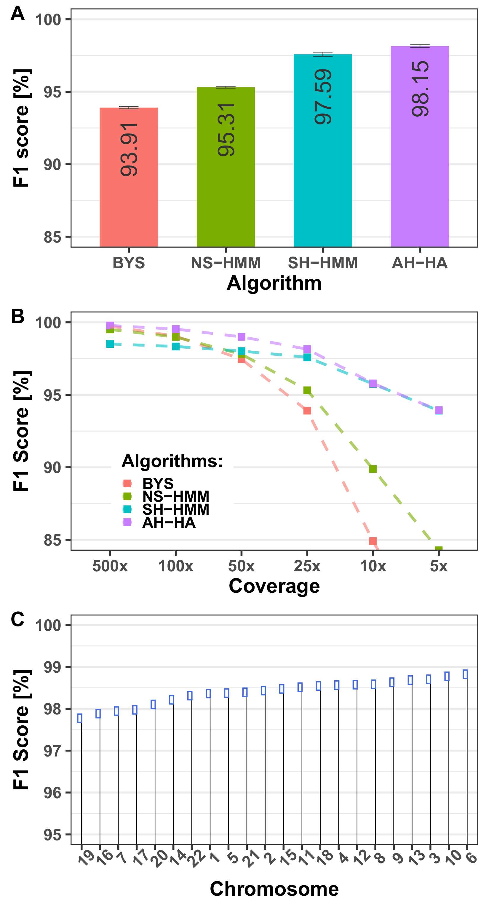
3.1.1. Algorithm Performance

To evaluate the performance of the different algorithms, the resulting inferred genotypes of these algorithms were summarized into an evaluation table. Table 2 shows the summarized results of AH-HA for the benchmark scenario: a 1:1 AJ–AJ mixed sample, chromosome 22, with 25× coverage and a 240 haplotype reference panel. The two genotypes (known and unknown) were divided into 9 scenarios, from which an F1 score was calculated (see Section 2.6). A number of key observations from this table:

a.

The AA–AA case accounts for 66.4% of all SNPs. This number is likely to remain high for all mixed samples. This case (together with the BB–BB case) is the simplest case of all algorithms, and hence the absolute performance of all algorithms is generally high.

b.

The unknown genotype is AA in 74.4% of all SNPs. A trivial algorithm that always outputs AA gives a good concordance score (74.4%), but an F1 score of 0 %. That is the main motivation behind using an F1 score instead of simple concordance.

c.

Two other simple inferences we looked at for baseline purposes are: 1. Infer the genotype most probable allele, based on the allele frequency of the reference panel for each SNP. This predictor yields an F1 score of 52.87% for the benchmark case. 2. Infer the genotype to be that of the known individual. This predictor yields an F1 score of 72.31% for the benchmark case.

AH-HA was compared with three other algorithms: (1) A per-SNP Bayesian algorithm (BYS), (2) a population-based Next SNP HMM (NS-HMM), and (3) a simple haplotype-based HMM (SH-HMM). See Section 2.4 for more details. Ten different realizations of the benchmark mixture were generated. These realizations differ both in the reads that enter each mixture and in the order in which the reference panel is organized (this order affects SH-HMM and AH-HA). All four algorithms were applied to the ten realizations. Figure 2A shows the average results of the four algorithms applied to these benchmark cases. There is a clear order that ranks the four algorithms, where SH-HMM and AH-HA outperform the two other algorithms. The P value is $<{10}^{-15}$, according to a t-test between AH-HA and NS-HMM or BYS. The simple predictors mentioned above, meant to serve as a baseline, performed much worse and are out of the presented scale of the figure.

Figure 2B shows the performance of the four algorithms for different mixture coverage values. AH-HA outperforms all other algorithms, for all coverage values (500×-5×). BYS performs well in high coverage scenarios (>100x), but, as coverage decreases, the per SNP prediction becomes less reliable. Even in high coverage scenarios, AH-HA achieves slightly better scoring, with 99.78% in 500× and 99.53% in 100×, compared with 99.74% and 99.04% scored by BYS. Compared with BYS, NS-HMM performs slightly better in lower coverage cases. This is due to the incorporation of allele statistics along the chromosome. However, also for NS-HMM, as coverage decreases, the performance significantly drops.

SH-HMM is outperformed by the above algorithms for high coverage scenarios (>100×), but for low coverage it utilizes the reference panel to attain better performance than BYS and NS-HMM, which score below 90%. In 10× coverage, SH-HMM scores 95.752%, while AH-HA has a 95.785% score, and in 5× coverage it scores 93.907%, lower than 93.936% scored by AH-HA. AH-HA combines two advantages: for low coverage, it utilizes the model through the reference panel, and for high coverage, it relies more on the observed allele count by its back-tracking phase. These features of AH-HA make it superior to all other algorithms considered here. It should be noted that forensic samples often suffer from degradation. Therefore, they will have low coverage and high error rates, emphasizing the need for reliable performance under these conditions. To test the robustness of AH-HA over the whole genome, we calculated its performance on the rest of the autosomal chromosomes (Figure 2C). AH-HA shows consistent performance across all chromosomes (10,355,283 total SNPs). The highest F1 score is 98.82% for chromosome 6 and the lowest is 97.77% for chromosome 19. Figure 2C shows that the score for chromosome 22 is close to the average, validating the benchmark mixture as a good indicator for a WGS case. The calculated F1 score of AH-HA of all chromosomes combined is 98.45%.

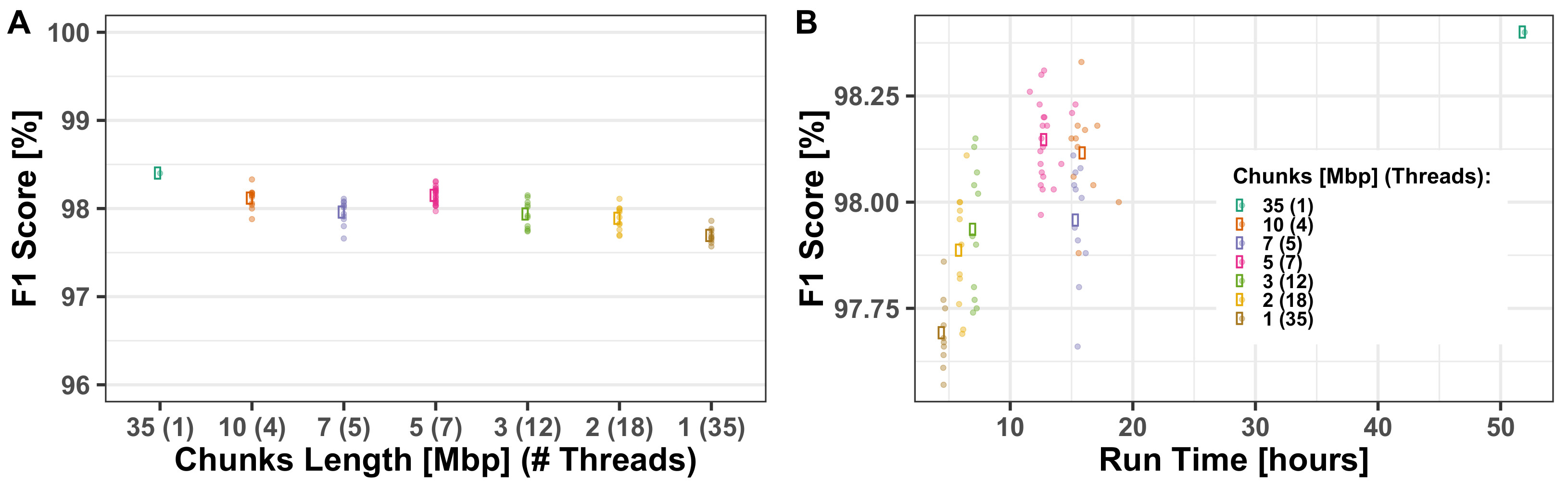
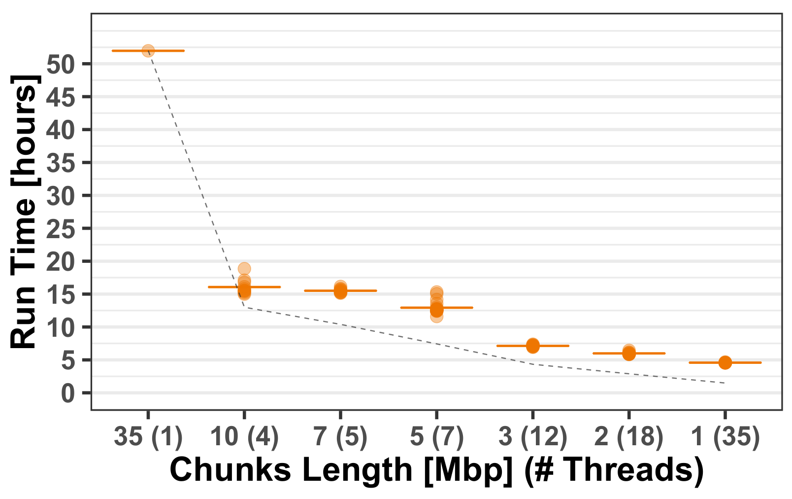
3.1.2. Computational Run-Times

SH-HMM and AH-HA have a relatively high computation cost, both in memory and in run time. In these algorithms, the Viterbi solver runs over all possible combinations for every SNP in the “Forward” stage. It utilizes a “two-dimensional” hidden state matrix that scales quadratically with panel size, i.e, assuming J haplotypes are used in the panel (240 for the standard case), with L total SNPs, the run-time scales like:

$$T_{run-time}\propto J\times J\times L$$

(3)

A naïve Viterbi implementation would have a running time proportional to $L\times J^4$, but using some computational features we brought it down to $L\times J^2$.

Running AH-HA on the entire chromosome 22 (~143 K SNPs) on one core of our server, Intel(R) Xeon(R) CPU E5-2670 v3 @ 2.30GHz (256GB memory), takes about 100 h. Even though emphasis is put on algorithm accuracy rather than efficiency, this runtime could be improved. In particular, when considering BYS and NS-HMM that perform the same task in about a minute on a home laptop (i5 processor, 8GB RAM). The first action that was taken is reducing the number of computations for each SNP (see also Appendix B). The second action was to use multi-threading. Whole chromosomes were split into non-overlapping segments of 5 Mbp.A comparison of run times of AH-HA for the benchmark case for different chunk lengths and, respectively, the number of threads running in parallel is shown in Figure 3. The theoretical decrease in runtime (1/#threads) is shown by the dashed line. The main reason for run times to differ from the expected values is that in practice, the total run time is determined by the segment with the largest number of SNPs. The default chunk length used, 5 Mbp, splits the ~143 K SNPs spread over 35 Mbp in chromosome 22 into 7 chunks. It manages to cut algorithm run time from about 50 h to around 13 h. Scoring was slightly affected by splitting. About a 0.5% point decrease in F1 score was seen between single thread performance and multi-thread performance. Within the multi-thread runs, performance has minor differences, varying within 0.25 percentage points, where the 5Mbp chunk-split has the highest average score (see Appendix A.1).

3.2. Model Configuration

3.2.1. HMM Parameters

Figure 4 shows AH-HA’s sensitivity to different model parameters. These parameters are estimated, as described in Section 2.5. Since $N_e$, $\theta$ and $ϵ$ are estimated, the goal was to test: (a) if these are optimal values, and (b) the effect each parameter has on the performance. F1 scores of AH-HA running the benchmark case were calculated with parameters in different orders of magnitude relative to the optimal estimated values (×10, ×1, and ×0.1). All combinations of ($N_e$, $\theta$, $ϵ$) values were tested. The initial estimation (×1) indeed obtains the best F1 score.

Larger $\theta$ and $ϵ$ values in the model do not negatively affect the F1 score so much. This can be attributed to the fact that higher values in these parameters correspond to higher probabilities of changes from the observed data. Another observation from Figure 4 is that even when the parameters are estimated wrongly, AH-HA remains fairly steady in terms of F1 score.

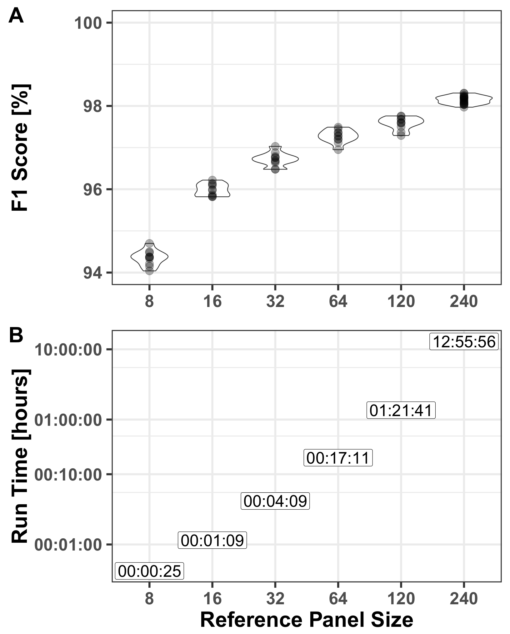
3.2.2. Reference Panel

Another important factor affecting AH-HA’s performance is the reference panel size. The benchmark scenario was run with varying panel sizes: 8, 16, 32, 64, 120, and 240 haplotypes. For each panel size, 10 realizations of J randomly chosen haplotypes from the 240 haplotypes in the AJ panel were used. For the full panel (240), haplotype order was randomized between the 10 realizations. The results in Figure 5 indicate how the choice of panel size affects the accuracy (Figure 5A) and run time (Figure 5B). There is a clear trade-off between the two. Running time scales quadratically with panel size, while the F1 score moderately increases with panel size. For example, decreasing the panel size from 240 to 120 (50%) cuts runtime by $89.5\%$, while the F1 score decreases only by 0.6 percentage points. The decrease from 240 to 8 (97%), lowers the runtime by 99.9% and reduces the F1 score by just 3.8% points, but scoring only a 0.5–1% points better than the naïve BYS algorithm. This could be a good trade-off for when run times and memory are a consideration.

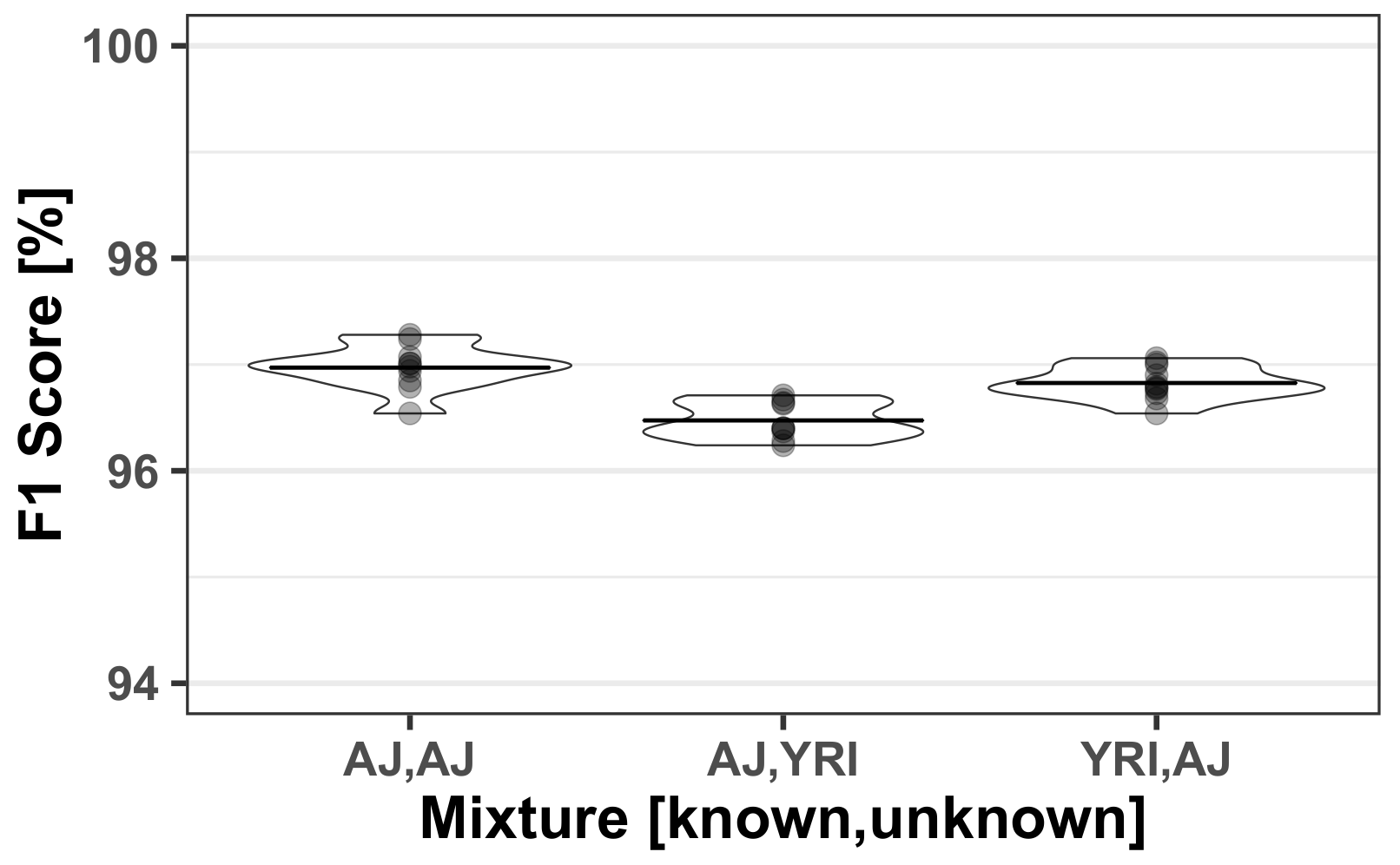
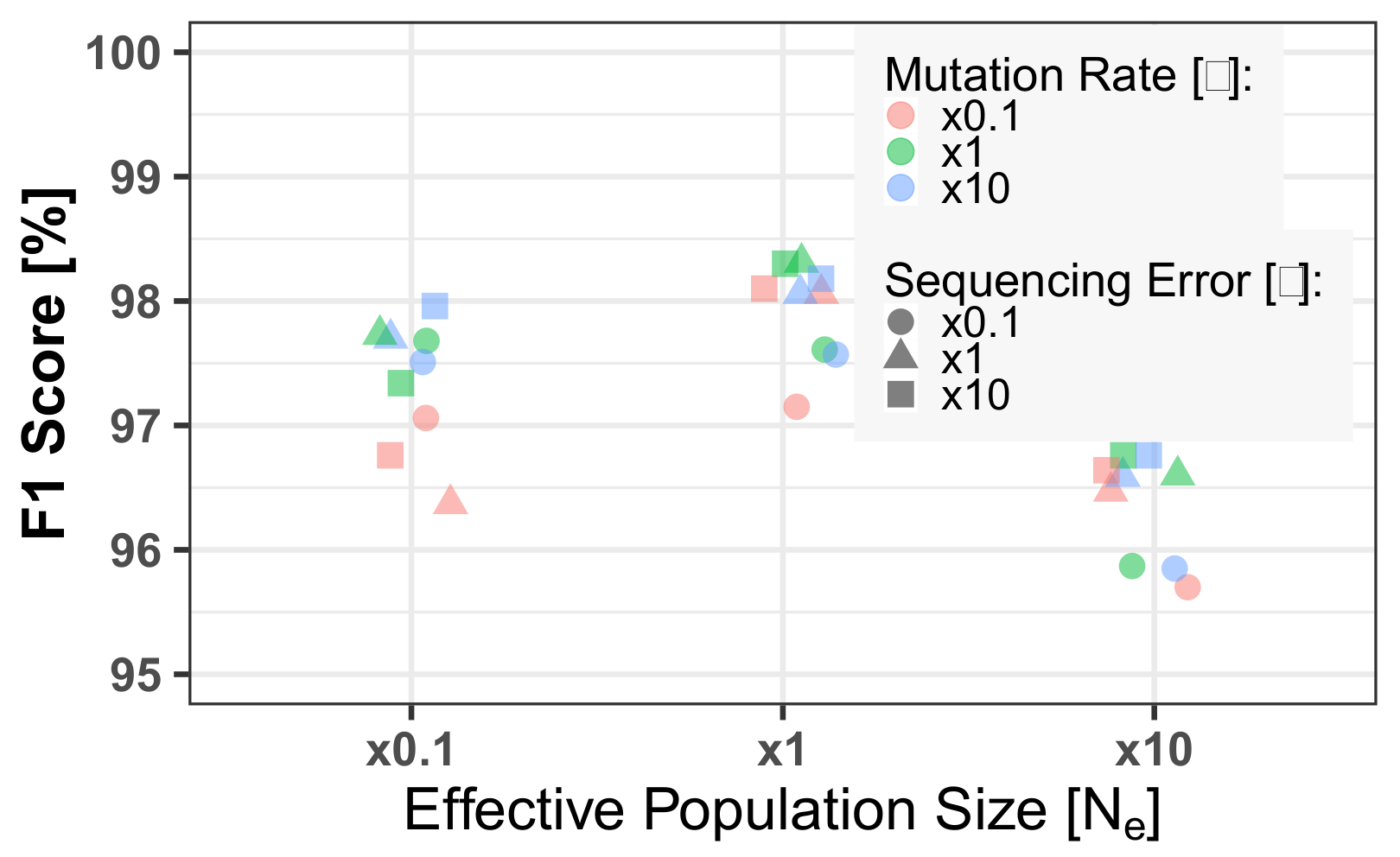
3.3. Mixed Population

We further tested AH-HA for different populations, to evaluate the effect on the algorithm’s performance when a mixture of donors of different origins is used, i.e., higher genetic diversity between individuals. Using data from the 1000 Genomes project, a mixture of a YRI individual (NA18489) and $A{J}_{father}$ was generated. Using a YRI-panel (constructed from these data as well, see Section 2.3), relevant values of $N_e$ and $\theta$ were calculated with CHROMOPAINTER ($N_e=1868.956$, $\theta$ = 1.797 × 10⁻⁴). The AJ-YRI mixture was processed by AH-HA, once with $A{J}_{father}$ as the unknown individual and once with NA18489 as the unknown. Each scenario was run over 10 realizations of the mixture with the unknown individual’s relevant panel, with randomly ordered haplotypes. Similarly, an AJ–AJ mixture of the same coverage with $A{J}_{father}$ as unknown was run by AH-HA. Figure 6 shows the scores for these three scenarios. AH-HA performs well for the AJ-YRI mixture in both configurations for the ancestry of the unknown individual and it is comparable to the AJ-AJ case, with a minor decrease in the average score.

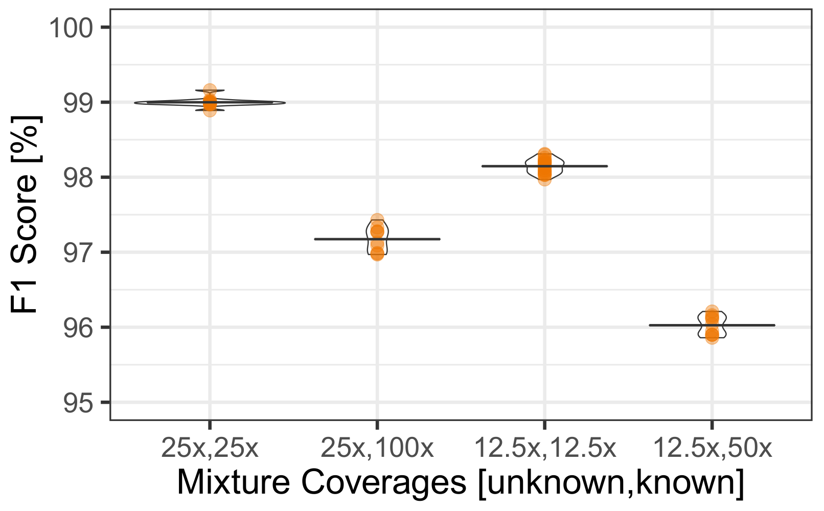
3.4. Uneven Mixtures

By modifying the calculation of the emission stage, AH-HA was adapted to analyze an uneven mixture of 20–80% (1:4 ratio) for the unknown and known individuals, respectively. Figure 7 shows a comparison of the results between a 1:1 mixture and a 1:4 mixture, for two coverage depths of the unknown contributor (25× and 12.5×). The results were generated from 10 randomly subsampled mixtures and 10 randomly ordered reference haplotypes. The uneven mixtures achieve lower F1 scores, about 1.8 percentage points below the 1:1 mixture (benchmark example), regardless of total coverage depths.

4. Discussion

In this paper we introduced AH-HA, an approach to infer the SNP profile of an unknown individual from an HTS of a mixed sample. It outperforms other methods’ F1 scores over varying coverage rates, as demonstrated in Figure 2B. In particular, the performance for low coverage is superior compared with more naïve algorithms, as shown in Section 3.1.1. The robustness of AH-HA was shown over all chromosomes, mixed population cases and different hyper-parameters. AH-HA’s run-time and memory was improved by utilizing multi-thread parallelization, splitting the chromosome into chunks and processing them simultaneously, as demonstrated in Section 3.1.2. The size of the reference panel strongly affects the run time but has a minor impact on the model’s performance, as demonstrated in Section 3.2.2. Consequently, AH-HA performs better than naïve methods, while maintaining comparable run times. Our approach uses two sources of information: one based only on read counts (without any LD consideration) and the other leaning heavily on LD. This means that when the read count for the observed allele is low, there is a higher weight to the LD model, essentially imputing the genotype.

Other algorithms dealing with SNPs in forensic DNA mixtures focus only on individual identification in a complex mixtures [14], mainly for inclusion or exclusion of a specific known individual from a mixture. For example, Voskoboinik et al. [21] showed that using 1000 SNPs with relatively low minor allele frequencies (~0.05–0.1), the presence of a known person in a ten-person mixture can be identified with high confidence. Ricke et al. [18] introduced a method that utilizes 2655 SNPs for identifying sub profiles from a mixture with uneven mixture ratios. These other algorithms focus on a different problem (identifying the presence of a known person). They are using a customized SNP panel of several thousand markers and require high coverage. AH-HA, on the contrary, works on hundreds of thousands of SNPs inferred from NGS data with moderate to low coverage (5×). Also, these algorithms require certain minor allele frequencies (MAF) in their data and uneven mixture ratios, while in AH-HA all of the called SNPs were used.

It should be mentioned that AH-HA will not match the whole genome sequence of the unknown/suspect even if the deconvolution is accurate, as it does not infer sites that are not in the reference panel, which may include variants that are individual-specific. In our case, sites not included in TAGC128 were excluded. If a site does not appear in TAGC128, everyone has the exact same allele. Such sites are not informative and do not affect the HMM. These excluded sites can still be inferred from the mixture using the naïve BYS algorithm.

AH-HA requires prior knowledge about the ethnic origin of the suspect and an accurate genotype of the victim. In case of unknown ancestry of the suspect, available forensic and investigative methods can be used, for example by searching for unique markers in the mixture that do not belong to the victim and are indicative for deducing ancestry [39,40].

Currently, AH-HA handles only bi-allelic SNPs, which are the majority of SNPs [23]. For uneven mixture ratios, assuming the ratio is deduced beforehand with another technique, the emission probabilities can be adjusted for the new ratios, as shown in Section 3.4 for a 1:4 case. AH-HA can confront noisy reads by changing $ϵ$. In case of an admixed unknown individual, we would need a multi-ancestry panel. Also, instead of the Viterbi solver that gives only the “best” path of the HMM, a softer solving method can be used. As discussed in Rabiner et al. [38], combining probabilities from the forward and backward stages the probability for each state value can be calculated, enabling a soft decision over all state values (per SNP) and even a “confidence” measure.

In mixtures with more than two individuals, when only one of them is unknown, AH-HA will require all known genotypes, and the emission step should be adapted accordingly. Extending AH-HA to infer more than one unknown individual is a greater challenge for the currently used HMM. First of all, computation wise, the algorithm will need to process for every SNP all combinations of haplotype pairs for every unknown individual. This will increase computation cost by two polynomial orders for each additional unknown individual. E.g., if we have two unknown individuals to infer from the mixture instead of one, AH-HA will effectively be calculating a 4D hidden state matrix (2 × 2) instead of a 2D matrix. In the case of all haplotypes coming from the same reference panel with J haplotypes, this would mean calculating and saving $J^4$ hidden state probabilities for each SNP. The second challenge is assignment of haplotypes to individuals. The algorithm infers four haplotypes, but without additional information on the target individuals, it is difficult to assign these haplotypes into two genotypes correctly.

AH-HA can be extended by exploring new implementation methods. First, incorporating “read-based” inference to the algorithm. This approach has the ability to accurately “stitch” SNPs from the same haplotype by overlapping read sequences (containing two or more SNPs) [41]. This will result in a better haplotype estimation for closely positioned SNPs, improving genotype inference. Second, inference can be made using the Markov chain Monte Carlo (MCMC) algorithm, similar to the method used by SHAPEIT [33]. This has the potential to improve run time and memory, but maintain accuracy. Another approach for improving run times could be to scale up from looking at per SNP states into using “representative” haplotype chunks as state values, similar to the method used in BEAGLE [42]. Also, adapting our model to fit the algorithm described by Lunter [43] and solve based on a positional Burrows–Wheeler transform may significantly improve run time and will be a subject of future research.

AH-HA requires HTS as input and currently cannot use cheaper SNP typing alternatives. Adapting it to using such alternatives may be doable, but it should be more difficult to perform deconvolution of the mixture using such data. This is because the available information is in the form of intensities (i.e., "analog" information vs. the "digital" information in sequencing).

AH-HA is built on the principles of the Li and Stephens model [28], which revolutionized phasing, imputation, and ancestry inference. However, in the context of DNA mixture analysis, this model’s potential has not been fully realized. AH-HA opens the door for future studies in DNA mixture analysis, which will develop as more and more HTS elements are being used for forensic work.

References

1. Gill, P. An assessment of the utility of single-nucleotide polymorphisms (SNPs) for forensic purposes. Int. J. Leg. Med. 2001, 114, 204–210. [Google Scholar] [CrossRef] [PubMed]
2. Sobrino, B.; Bríon, M.; Carracedo, A. SNPs in forensic genetics: A review on SNP typing methodologies. Forensic Sci. Int. 2005, 154, 181–194. [Google Scholar] [CrossRef] [PubMed]
3. Butler, J.M.; Coble, M.D.; Vallone, P.M. STRs vs. SNPs: Thoughts on the future of forensic DNA testing. Forensic Sci. Med. Pathol. 2007, 3, 200–205. [Google Scholar] [CrossRef]
4. Butler, J.M.; Budowle, B.; Gill, P.; Kidd, K.; Phillips, C.; Schneider, P.M.; Vallone, P.; Morling, N. Report on ISFG SNP panel discussion. Forensic Sci. Int. Genet. Suppl. Ser. 2008, 1, 471–472. [Google Scholar] [CrossRef]
5. Algee-Hewitt, B.F.; Edge, M.D.; Kim, J.; Li, J.Z.; Rosenberg, N.A. Individual identifiability predicts population identifiability in forensic microsatellite markers. Curr. Biol. 2016, 26, 935–942. [Google Scholar] [CrossRef] [PubMed] [Green Version]
6. Liu, Y.Y.; Harbison, S. A review of bioinformatic methods for forensic DNA analyses. Forensic Sci. Int. Genet. 2018, 33, 117–128. [Google Scholar] [CrossRef] [PubMed]
7. Budowle, B.; Van Daal, A. Forensically relevant SNP classes. Biotechniques 2008, 44, 603–610. [Google Scholar] [CrossRef] [PubMed] [Green Version]
8. Daniel, R.; Santos, C.; Phillips, C.; Fondevila, M.; Van Oorschot, R.; Carracedo, A.; Lareu, M.; McNevin, D. A SNaPshot of next generation sequencing for forensic SNP analysis. Forensic Sci. Int. Genet. 2015, 14, 50–60. [Google Scholar] [CrossRef] [PubMed]
9. Churchill, J.D.; Schmedes, S.E.; King, J.L.; Budowle, B. Evaluation of the Illumina® beta version ForenSeq™ DNA signature prep kit for use in genetic profiling. Forensic Sci. Int. Genet. 2016, 20, 20–29. [Google Scholar] [CrossRef]
10. Erlich, Y.; Shor, T.; Pe’er, I.; Carmi, S. Identity inference of genomic data using long-range familial searches. Science 2018, 362, 690–694. [Google Scholar] [CrossRef] [Green Version]
11. Katsanis, S.H. Pedigrees and perpetrators: Uses of DNA and genealogy in forensic investigations. Annu. Rev. Genom. Hum. Genet. 2020, 21, 535–564. [Google Scholar] [CrossRef] [PubMed] [Green Version]
12. Kennett, D. Using genetic genealogy databases in missing persons cases and to develop suspect leads in violent crimes. Forensic Sci. Int. 2019, 301, 107–117. [Google Scholar] [CrossRef] [PubMed]
13. Gettings, K.B.; Kiesler, K.M.; Vallone, P.M. Performance of a next generation sequencing SNP assay on degraded DNA. Forensic Sci. Int. Genet. 2015, 19, 1–9. [Google Scholar] [CrossRef] [PubMed]
14. Yang, J.; Lin, D.; Deng, C.; Li, Z.; Pu, Y.; Yu, Y.; Li, K.; Li, D.; Chen, P.; Chen, F. The advances in DNA mixture interpretation. Forensic Sci. Int. 2019. [Google Scholar] [CrossRef] [PubMed]
15. Buckleton, J.S.; Bright, J.A.; Gittelson, S.; Moretti, T.R.; Onorato, A.J.; Bieber, F.R.; Budowle, B.; Taylor, D.A. The Probabilistic Genotyping Software STR mix: Utility and Evidence for its Validity. J. Forensic Sci. 2019, 64, 393–405. [Google Scholar] [CrossRef]
16. Haned, H.; Slooten, K.; Gill, P. Exploratory data analysis for the interpretation of low template DNA mixtures. Forensic Sci. Int. Genet. 2012, 6, 762–774. [Google Scholar] [CrossRef]
17. Bleka, Ø.; Storvik, G.; Gill, P. EuroForMix: An open source software based on a continuous model to evaluate STR DNA profiles from a mixture of contributors with artefacts. Forensic Sci. Int. Genet. 2016, 21, 35–44. [Google Scholar] [CrossRef] [Green Version]
18. Ricke, D.O.; Isaacson, J.; Watkins, J.; Fremont-Smith, P.; Boettcher, T.; Petrovick, M.; Wack, E.; Schwoebel, E. The Plateau Method for Forensic DNA SNP Mixture Deconvolution. bioRxiv 2017, 225805. [Google Scholar]
19. Gill, P.; Haned, H.; Eduardoff, M.; Santos, C.; Phillips, C.; Parson, W. The open-source software LRmix can be used to analyse SNP mixtures. Forensic Sci. Int. Genet. Suppl. Ser. 2015, 5, e50–e51. [Google Scholar] [CrossRef] [Green Version]
20. Bleka, Ø.; Eduardoff, M.; Santos, C.; Phillips, C.; Parson, W.; Gill, P. Open source software EuroForMix can be used to analyse complex SNP mixtures. Forensic Sci. Int. Genet. 2017, 31, 105–110. [Google Scholar] [CrossRef]
21. Voskoboinik, L.; Ayers, S.B.; LeFebvre, A.K.; Darvasi, A. SNP-microarrays can accurately identify the presence of an individual in complex forensic DNA mixtures. Forensic Sci. Int. Genet. 2015, 16, 208–215. [Google Scholar] [CrossRef] [PubMed]
22. Isaacson, J.; Schwoebel, E.; Shcherbina, A.; Ricke, D.; Harper, J.; Petrovick, M.; Bobrow, J.; Boettcher, T.; Helfer, B.; Zook, C.; et al. Robust detection of individual forensic profiles in DNA mixtures. Forensic Sci. Int. Genet. 2015, 14, 31–37. [Google Scholar] [CrossRef] [PubMed]
23. Campbell, I.M.; Gambin, T.; Jhangiani, S.N.; Grove, M.L.; Veeraraghavan, N.; Muzny, D.M.; Shaw, C.A.; Gibbs, R.A.; Boerwinkle, E.; Yu, F.; et al. Multiallelic positions in the human genome: Challenges for genetic analyses. Hum. Mutat. 2016, 37, 231–234. [Google Scholar] [CrossRef] [PubMed]
24. Kidd, K.; Pakstis, A.; Speed, W.; Lagace, R.; Chang, J.; Wootton, S.; Ihuegbu, N. Microhaplotype loci are a powerful new type of forensic marker. Forensic Sci. Int. Genet. Suppl. Ser. 2013, 4, e123–e124. [Google Scholar] [CrossRef]
25. Voskoboinik, L.; Motro, U.; Darvasi, A. Facilitating complex DNA mixture interpretation by sequencing highly polymorphic haplotypes. Forensic Sci. Int. Genet. 2018, 35, 136–140. [Google Scholar] [CrossRef]
26. Zhu, S.J.; Almagro-Garcia, J.; McVean, G. Deconvolution of multiple infections in Plasmodium falciparum from high throughput sequencing data. Bioinformatics 2018, 34, 9–15. [Google Scholar] [CrossRef] [Green Version]
27. Smart, U.; Cihlar, J.C.; Mandape, S.N.; Muenzler, M.; King, J.L.; Budowle, B.; Woerner, A.E. A continuous statistical phasing framework for the analysis of forensic mitochondrial DNA mixtures. Genes 2021, 12, 128. [Google Scholar] [CrossRef]
28. Li, N.; Stephens, M. Modeling linkage disequilibrium and identifying recombination hotspots using single-nucleotide polymorphism data. Genetics 2003, 165, 2213–2233. [Google Scholar] [CrossRef]
29. Lawson, D.J.; Hellenthal, G.; Myers, S.; Falush, D. Inference of population structure using dense haplotype data. PLoS Genet. 2012, 8, e1002453. [Google Scholar] [CrossRef] [Green Version]
30. Browning, S.R.; Browning, B.L. Haplotype phasing: Existing methods and new developments. Nat. Rev. Genet. 2011, 12, 703–714. [Google Scholar] [CrossRef] [Green Version]
31. Howie, B.; Marchini, J.; Stephens, M. Genotype imputation with thousands of genomes. G3 Genes Genomes Genet. 2011, 1, 457–470. [Google Scholar] [CrossRef] [PubMed] [Green Version]
32. 1000 Genomes Project Consortium. An integrated map of genetic variation from 1,092 human genomes. Nature 2012, 491, 56. [Google Scholar] [CrossRef] [PubMed] [Green Version]
33. Delaneau, O.; Zagury, J.F.; Marchini, J. Improved whole-chromosome phasing for disease and population genetic studies. Nat. Methods 2013, 10, 5–6. [Google Scholar] [CrossRef] [PubMed]
34. Carmi, S.; Hui, K.Y.; Kochav, E.; Liu, X.; Xue, J.; Grady, F.; Guha, S.; Upadhyay, K.; Ben-Avraham, D.; Mukherjee, S.; et al. Sequencing an Ashkenazi reference panel supports population-targeted personal genomics and illuminates Jewish and European origins. Nat. Commun. 2014, 5, 4835. [Google Scholar] [CrossRef] [PubMed] [Green Version]
35. Zook, J.M.; Catoe, D.; McDaniel, J.; Vang, L.; Spies, N.; Sidow, A.; Weng, Z.; Liu, Y.; Mason, C.E.; Alexander, N.; et al. Extensive sequencing of seven human genomes to characterize benchmark reference materials. Sci. Data 2016, 3. [Google Scholar] [CrossRef] [Green Version]
36. Wall, J.D.; Tang, L.F.; Zerbe, B.; Kvale, M.N.; Kwok, P.Y.; Schaefer, C.; Risch, N. Estimating genotype error rates from high-coverage next-generation sequence data. Genome Res. 2014, 24, 1734–1739. [Google Scholar] [CrossRef] [Green Version]
37. Gibbs, R.A.; Belmont, J.W.; Hardenbol, P.; Willis, R.A.; Gibbs, T.D.; Yu, F.L.; Yang, H.M.; Ch’ang, L.Y.; Huang, W.; Liu, B.; et al. The international HapMap project. Nature 2003, 426, 789–796. [Google Scholar] [CrossRef] [Green Version]
38. Rabiner, L.R. A tutorial on hidden Markov models and selected applications in speech recognition. Proc. IEEE 1989, 77, 257–286. [Google Scholar] [CrossRef] [Green Version]
39. Kidd, K.K.; Speed, W.C.; Pakstis, A.J.; Furtado, M.R.; Fang, R.; Madbouly, A.; Maiers, M.; Middha, M.; Friedlaender, F.R.; Kidd, J.R. Progress toward an efficient panel of SNPs for ancestry inference. Forensic Sci. Int. Genet. 2014, 10, 23–32. [Google Scholar] [CrossRef] [Green Version]
40. Wei, Y.L.; Wei, L.; Zhao, L.; Sun, Q.F.; Jiang, L.; Zhang, T.; Liu, H.B.; Chen, J.G.; Ye, J.; Hu, L.; et al. A single-tube 27-plex SNP assay for estimating individual ancestry and admixture from three continents. Int. J. Leg. Med. 2016, 130, 27–37. [Google Scholar] [CrossRef]
41. Delaneau, O.; Howie, B.; Cox, A.J.; Zagury, J.F.; Marchini, J. Haplotype estimation using sequencing reads. Am. J. Hum. Genet. 2013, 93, 687–696. [Google Scholar] [CrossRef] [PubMed] [Green Version]
42. Browning, S.R.; Browning, B.L. Rapid and accurate haplotype phasing and missing-data inference for whole-genome association studies by use of localized haplotype clustering. Am. J. Hum. Genet. 2007, 81, 1084–1097. [Google Scholar] [CrossRef] [PubMed] [Green Version]
43. Lunter, G. Haplotype matching in large cohorts using the Li and Stephens model. Bioinformatics 2019, 35, 798–806. [Google Scholar] [CrossRef] [PubMed]
Figure 1. An outline of AH-HA. A mixed sequenced sample ( N ) is processed together with a reference panel ( H ) and a known donor genotype ( G k n o w n ) in a Hidden Markov Model (HMM). The output is an inferred genotype of the unknown donor.
Forensicsci 02 00034 g001
Figure 2. Performance comparison. F1 scores (Y-axis) are shown: (A) for the benchmark scenario (AJ–AJ, 1:1, depth 25×) for each algorithm as indicated by the X-axis. Error bars represent the total variation between 10 random mixtures. (B) For varying sequencing coverage (X-axis) for the four algorithms (different colors as indicated in the legends). Y-axis was scaled, to improve the resolution of the differences between the graphs. (C) For AH-HA over all autosomal chromosomes (X-axis). Chromosomes are ordered by their F1 score.
Forensicsci 02 00034 g002
Figure 3. Algorithm run-times. AH-HA run times are shown for different chunk sizes and thread count for the benchmark scenario. Average values (in hours) are indicated by a horizontal line. Theoretical, optimized run time is shown by the dashed line. All runs were conducted on an Intel(R) Xeon(R) CPU E5-2670 v3 @ 2.30GHz server with 48 cores and 256 GB memory.
Forensicsci 02 00034 g003
Figure 4. Parameter selection effect. F1 scores (Y axis) are shown for different AH-HA parameters for the benchmark scenario. The indicated fold change values refer to the fitted values of the parameters as described in the methods. N e values follow the X axis labels, θ is indicated by color, and ϵ is indicated by symbol shapes.
Forensicsci 02 00034 g004
Figure 5. Panel size effect. F1 scores (Y-axis in A) and mean run-times (Y-axis in B) are shown for varying reference panel sizes (X-axis) for the AJ–AJ mixture. The different panels were created by sampling haplotypes from the AJ-panel (Section 2.2).
Forensicsci 02 00034 g005
Figure 6. YRI-AJ Mixtures. F1 scores (Y-axis) are shown for different population mixtures (X-axis). Performance was evaluated on chromosome 20 with coverage 18x. Mean value for each mixture is indicated by a horizontal line.
Forensicsci 02 00034 g006
Figure 7. Uneven Mixture. F1 scores (Y-axis) are shown for 1:1 and 1:4 mixture ratios (X-axis). Mean value of the F1 score in each mixture is indicated by a horizontal line.
Forensicsci 02 00034 g007