Durability Prediction of Cyclically Loaded CP-W800 Fillet Welds

Abstract

Two methods of durability prediction of fillet welds were researched in this study. Namely, the structural Hot-Spot method and the structural stress method fe-safe Verity were applied to fatigue life estimation of a double plate lap fillet weld made of high-strength complex phase CP-W800 steel. Durability predictions were compared against available high-cycle fatigue experimental data obtained for the same weld detail and material. Both 2D and 3D finite element meshes were considered in the simulations. It was shown that comparable predictions were obtained using either the Hot-Spot method or the fe-safe Verity module in the case of the 3D FE mesh. On the contrary, a less conservative durability prediction was observed using the Hot-Spot method and a more conservative durability prediction was gained using the fe-safe Verity module in the case of the 2D FE mesh due to a different consideration of stress concentration around the weld.

1. Introduction

Welding is an extensively used technology for joining steel metal components as the procedure is cost effective, it can be automated and allows design flexibility together with weight savings and high structural strength [1]. Welds are mainly made by a localized heat intensive process of melting together two or more adjacent components, e.g., by shielded metal arc, gas metal arc or plasma arc welding technology [2]. After the cool-down, they stay permanently bound as one part. Welding, however, is in fact also a very demanding and highly localized metallurgical process that significantly alters material microstructure, subsequently creating complex inhomogeneous regions of residual tensile stresses and deformation of original geometry [3]. The most important issue regarding the welds and welded structure, in comparison to base material, is considerable decrease in dynamic strength and fatigue life [4]. Inevitably, welds are considered weak spots of the structure by default, thus requiring proper design for durability considerations and separate empirical validations. After decades of research and a number of developed approaches for prediction of fatigue life of welded joints [5], the topic remains appealing.

Stress concentrations are the most important quantity when considering fatigue life calculations of welded joints. Stresses can be obtained experimentally, analytically and/or numerically, but in any of the three cases the task is not straightforward [6] as the demanding and complex estimations should involve reproduceable material and geometric data, exact process parameters, stress field inconsistencies and material inhomogeneities [7], to name only a few. In many real cases the data are missing or cannot be measured and remain unknown. In such cases, their impact on durability of a welded structure is considered indirectly, for instance, by intensification factors [4] representing many experimental data, as is the case with international standards covering the field, such as DIN 15018 [8] or more recent EN 1993-1-8 Eurocode 3 [9] and ASTM Standards for Welding (4th Edition) [10]. According to Hobbacher [11], the International Institute of Welding (IIW), a leading authority in developing and promoting material joining technologies, proposed four main methods for consistent fatigue life calculations based on available data and level of calculation effort, namely the Nominal stress approach (average stress in a welded joint with special fatigue data for each structural detail), Structural/geometrical “hot-spot” stress approach (considering stress types and stress components, obtained by finite element analysis (FEA)), Effective notch stress approach (calculation of notch stresses, but sensitive to the weld toe and the root design and finite element analysis) and Linear elastic fracture mechanical crack growth approach (based on concepts of fracture mechanics with limitation of practical application). What should be considered is the level of effort increase from the nominal stress approach towards the crack growth approach as concluded by Łagoda et al. [5], whereas effectiveness of all approaches decreases with complexity of the evaluated structure.

The structural hot-spot stress method is perhaps the most widely used by mechanical and design engineers [12,13] as it considers stress type and stress tensor components which is valid for fatigue evaluations and in general. Essentially, it is applicable to weld details where fatigue failure potentially starts from the weld toe [14,15]. The relevant stress at the weld toe is denoted as the “hot-stress” that is extrapolated from the nominal (structural) surface stresses to the weld toe. Nominal stresses can be measured or more commonly calculated at a reference point outside of the stress concentration zone of the detail by finite element analysis (FEA) [11,12]. Afterwards, fatigue life can be calculated by matching the hot-spot stress with the corresponding number of cycles given by relevant hot-spot stress empirical S-N curves [5].

The main limitations of discrete calculation FE methods for evaluation of nominal stresses are mostly connected to mesh and element sensitivity, numerical issues with singularities and algorithm stability at geometrical discontinuities and at stress concentrations [16]. This, unfortunately, is the opposite of what one would expect for weld analysis. To overcome mesh sensitivity issues, Dong [17] introduced an alternative finite element method based on the mapping of balanced nodal forces and moments along the evaluated weld line into equivalent structural stresses. The main advantage of the method is mesh-insensitive calculation of nodal stresses that in turn allows more convenient representation of a complex stress state due to weld notch effects. In addition, the approach also includes the formation of a universal master S-N curve [18,19], effectively replacing the need for weld-specific S-N curves. Since then, the method has been extensively tested and adopted in fatigue codes by ASME as well as included in commercial FE software Abaqus 2021 as a fe-safe Verity^®module [20,21].

The purpose of this work is focused on the understanding of the practical value of two established methods, namely the structural Hot-Spot method and the structural stress method fe-safe Verity, for fatigue life estimation of a double plate lap fillet weld made of high-strength complex phase CP-W800 steel, emphasizing the benefits and weaknesses of each method from an engineering point of view. The results of the research are validated with high-cycle S-N experimental data obtained for the actual weld detail and material [22].

2. Method

The method is divided into four parts. First, the experimental background is given. Next, the modelling part of the study is presented. Furthermore, the structural stress method fe-safe Verity is described, and finally, the structural Hot-Spot method is presented.

2.1. Experimental Background

The aim of the research is to estimate the duration of fillet welds in axially loaded joints between sheet metals. Fillet welds between the sheet metals can be created with an overlapping joint as given in Figure 1. However, a significant additional moment is introduced in the weld this way due to the asymmetry in simple (one-sided) overlapping joints. Namely, a lever for the moment is formed as a result of overlapping sheets on top of each other.

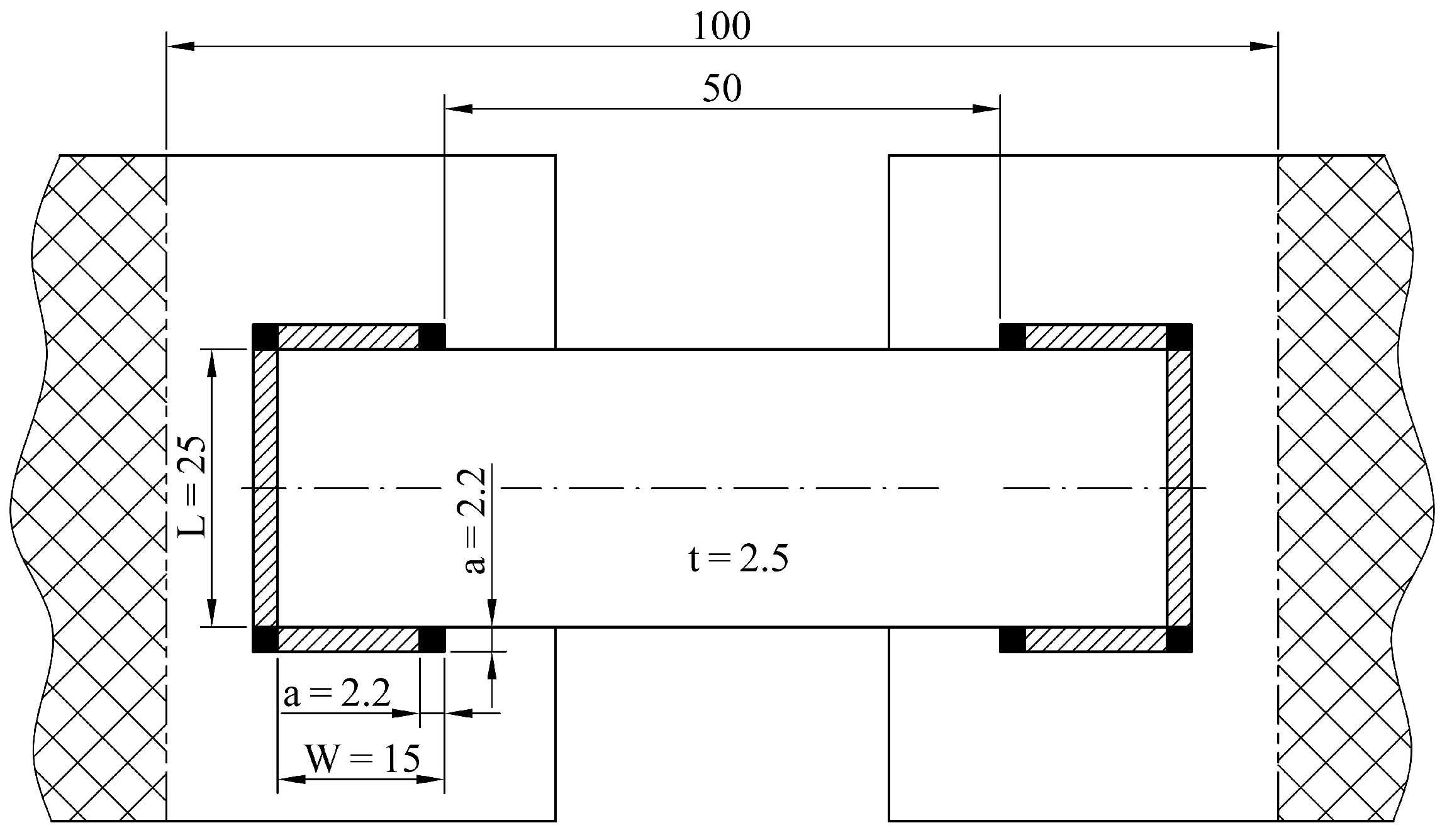
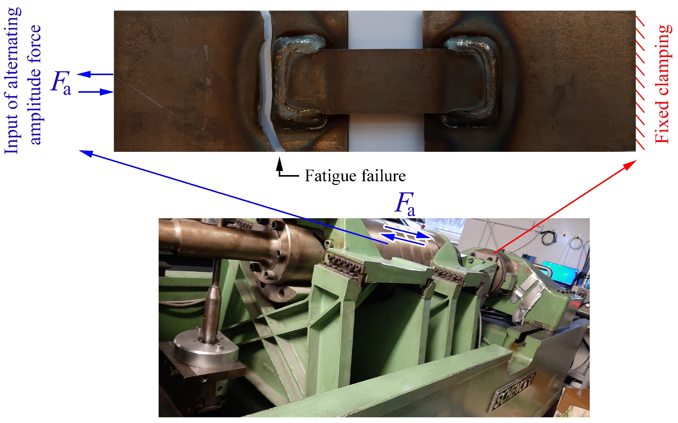
To circumvent this problem, a new symmetrical specimen with a two-sided overlapping joint was created, which can be seen in Figure 2 (above). In this case, two narrower longitudinal sheets were welded with fillet welds onto wider plates. These were then gripped by the clamps of the test rig SCHENCK intended for cyclic tests of material (Figure 2 below). One side of the test rig provided fixed (immovable) clamping and the other side introduced tensile/compressive load cycles into the specimen.

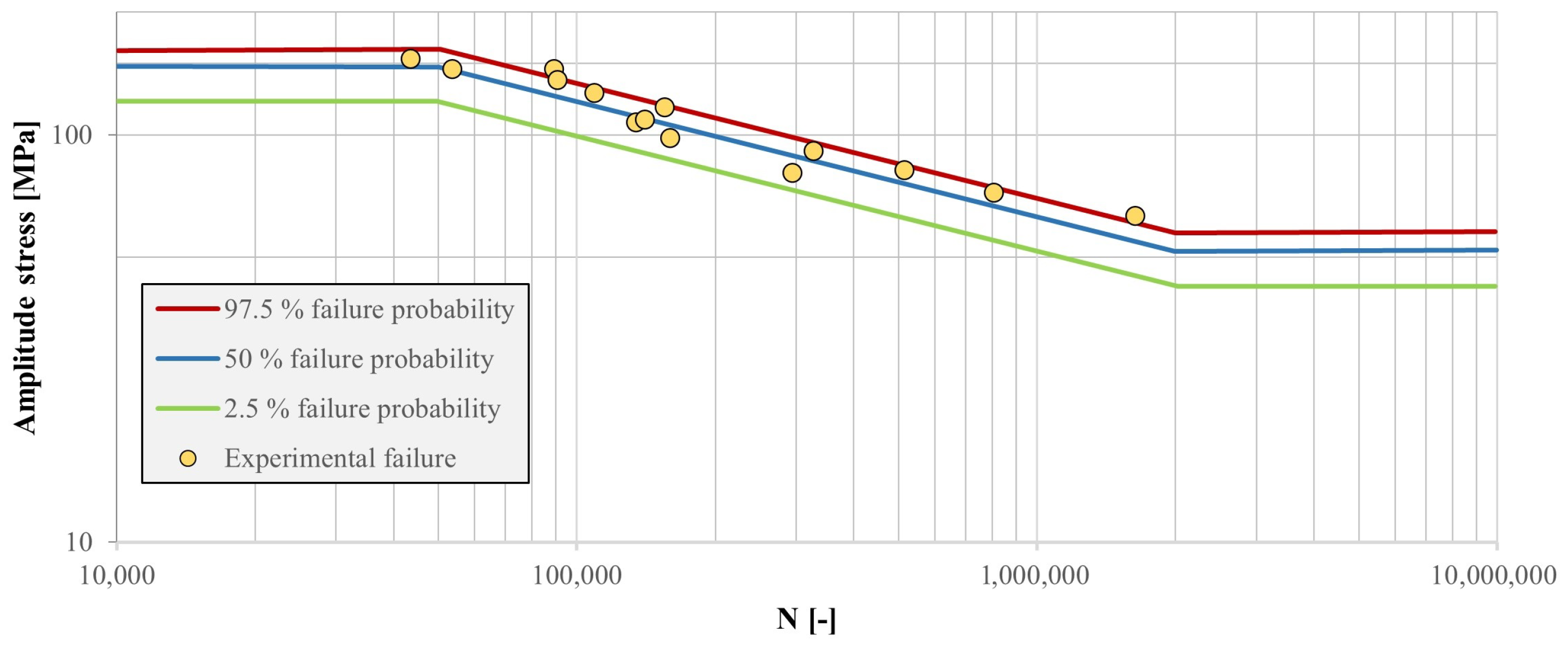
In this study, the following conditions were considered. The specimens were made of CP-W800 steel, welded together, placed into the test rig and subjected to pure alternating force-controlled cycle loading with a set of pre-determined force amplitudes and a sinusoidal form of the loading signal. The number of cycles to failure were recorded for each specimen, and then the durability curve was created. It is given in Figure 3.

The intention of the simulations, however, was to compare the simulated number of cycles to failure to experimental observations for a specific level of the loading signal. Force amplitude $F_{\mathrm{a}}=11\mathrm{kN}$ was thus considered, where the experimental specimen endured 159,298 cycles before failure. The shape of fatigue fracture occurring behind the transverse weld of the specimen can be seen in Figure 2 (above).

2.2. FE Modelling

Simulated durability prediction was carried out using software tools from Dassault Systèmes group. Both 3D and 2D models of the specimen were first created using Catia V5. We note that the 2D model is a shell mesh of the geometric model of the specimen. Next, the geometries were imported into Abaqus, where structural FE analyses were carried out. Finally, durability predictions were performed using fe-safe Verity. The latter is a special module within fe-safe environment intended for fatigue analysis of welds. As the tools are fully compatible, quick adjustments and easy entries of subsequent changes at any stage of calculation are possible, which saves a lot of time during evaluations. 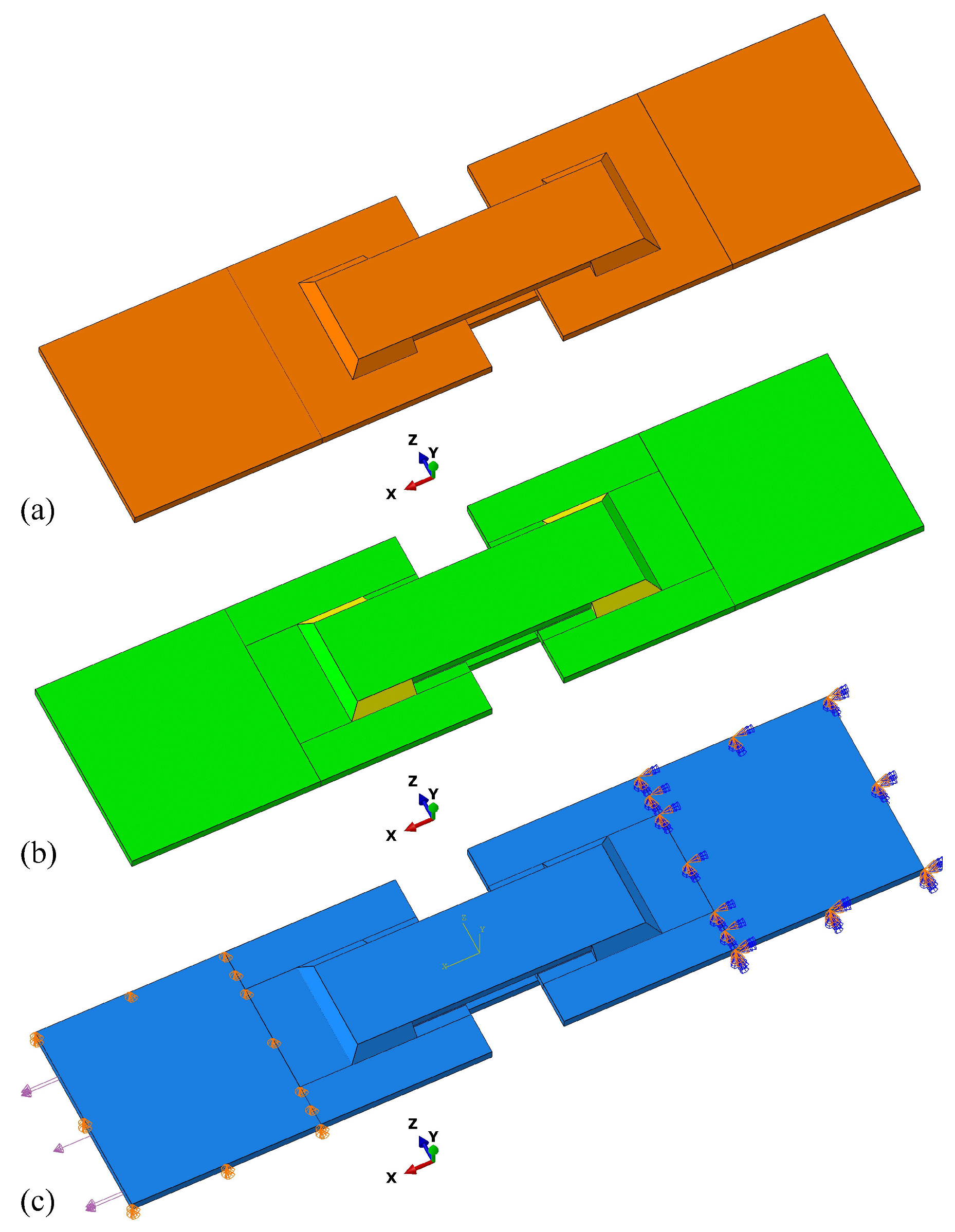Figure 4a shows the imported 3D geometry of the specimen via the .CATPart format into Abaqus. The experimental specimen and the virtual specimen for FE simulations were identical. This also included the geometric details such as the gap between the sheets, i.e., the sheets were spaced 0.6 mm apart, so the only load-bearing connections between the sheets were the welds. The input form of the part is important as it ensures full nodal connections between finite elements during the meshing process. FE mesh suitability was first assessed by the Mesh Controls command. Processing of various solid areas was based on colour scales which provided an insight into the current state of the geometry suitability. The orange-coloured solid area (Figure 4a) indicates the basic optional meshing of the entire geometry with tetrahedra, where only a random mesh of solid finite elements can be generated. However, since a structured mesh of hexahedra is preferable for the fe-safe Verity module, additional partitions were introduced to the geometric model of the welds. A structured FE mesh was thus obtained by forming symmetrical zones of the weld. Specifically, the external shapes of the welds were kept, but the structure of the geometry of the connected areas was changed in such a way that the previous single-piece 3D solid was then divided into individual symmetrical areas. These were then recognised by the automatic algorithm for structured meshing. In Figure 4, the transition from the initial state to the improved state can be seen. The green solid areas show the full capability for structured meshing where Hex or Hex-dominated finite element mesh can be generated. Similarly, the yellow solid areas indicate the intermediate capability for structured meshing where the Sweep function can be used for the generation of finite element mesh. The latter option is also appropriate for the definition of welds in fe-safe Verity. 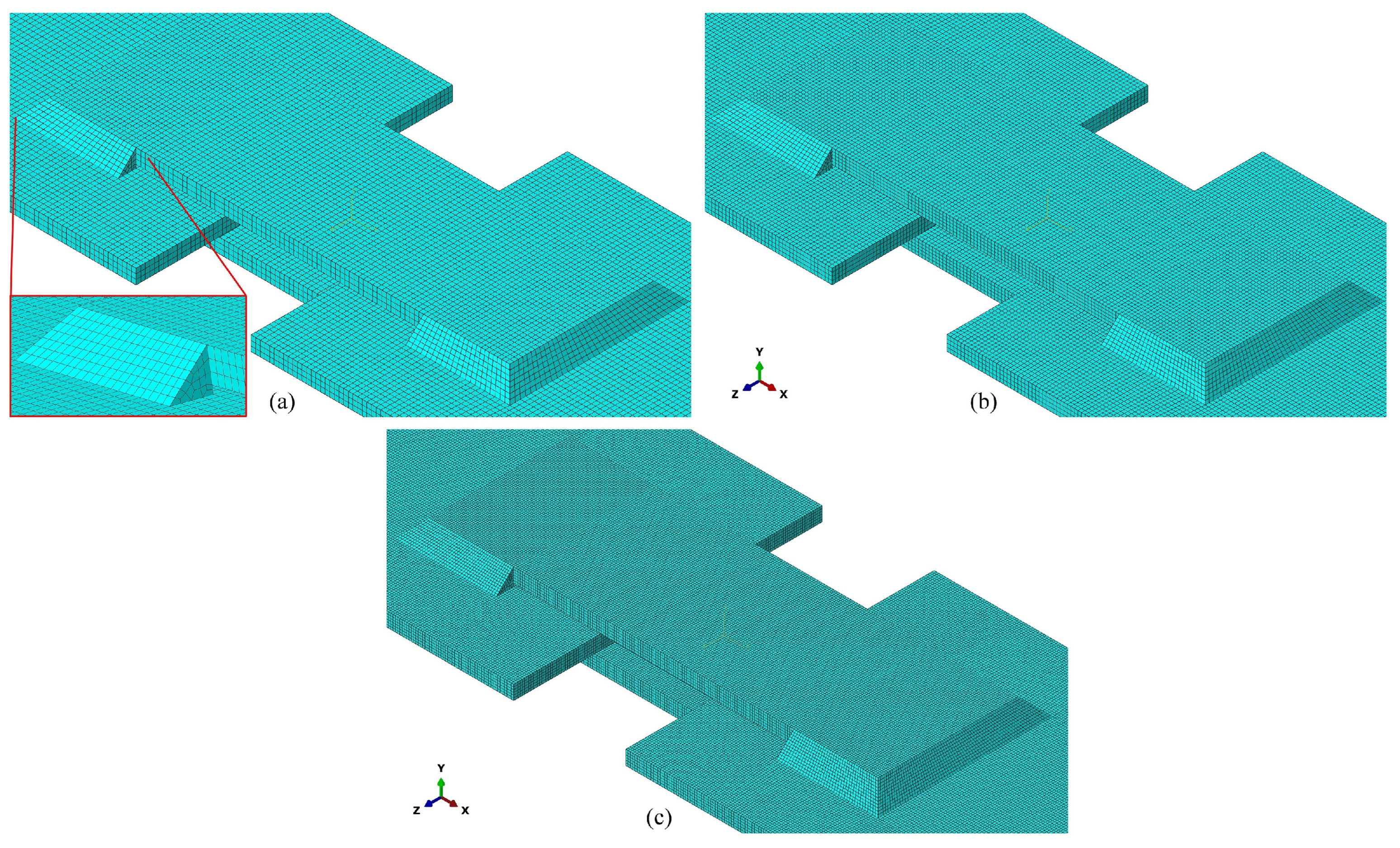As the structural Hot-Spot method requires the size of finite elements below the thickness of the thinnest sheet metal in the joint, but recommends the size below 40% of this value [11], the latter recommendation was used to determine the sizes of the coarse 3D mesh (0.83 mm) and 2D mesh (1 mm) in this study. The element sizes of the medium and fine 3D meshes were chosen as 0.5 mm 0.42 mm, respectively. The results of meshing the solid geometry of the specimen are given in Figure 5. From the generated FE models of finite elements, it can be seen that the welds and sheets are connected directly node to node via adjacent finite elements. The FE meshes consist of C3D8 type FE elements in the case of the 3D mesh and S4 in case of the 2D mesh. The number of elements and nodes for three 3D FE densities and the 2D mesh are given in

Table 1. Mesh properties of the generated FE models.

Mesh Density	No. of Elements	No. of Nodes
3D rough	78,620	105,852
3D medium	191,849	238,406
3D fine	622,092	730,377
2D	16,567	16,265

).

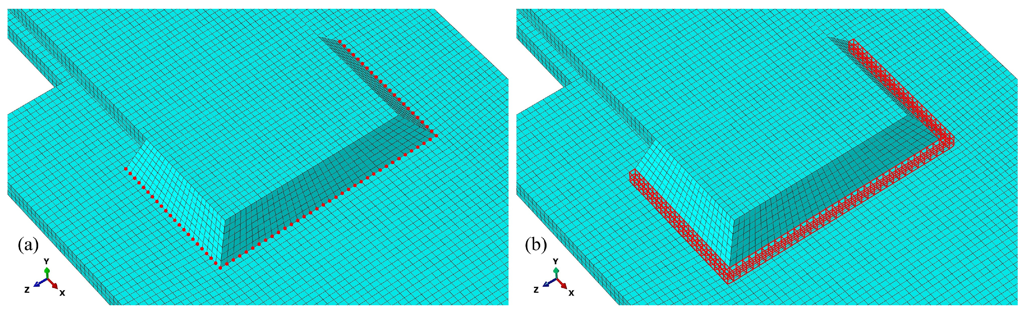
Finally, the supports and loads were defined to resemble experimental conditions (Figure 4c). On one side, the specimen was clamped, and on the other side, a pure alternating mechanical load was applied. As small finite element models were used in the analyses, the symmetry boundary conditions were not applied. However, for models with a greater number of finite elements, the consideration of the symmetry boundary conditions could also be considered. Importantly, node sets and finite element sets were created around all four fillet welds of the test specimen to identify them easily in the fe-safe Verity module during durability calculation (Figure 6).

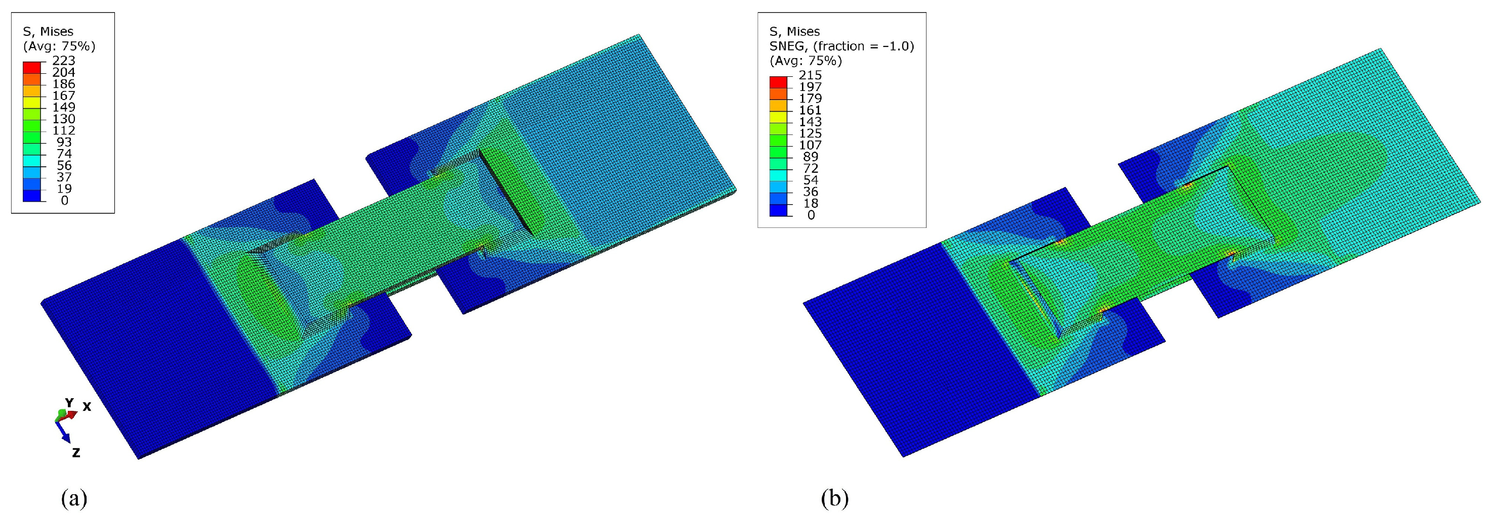
During the simulations, elastic modulus E = 200,000 MPa and Poisson’s ratio $\nu$ = 0.3 were taken into account for CP-W800 steel. Standard implicit structural analyses were performed, which served for the definition of the magnitudes of the maximum stresses and their location around the weld points.

2.3. Structural Stress Method FE-Safe Verity

The mesh-insensitive structural stress method was first proposed by Dong [17]. The approach adopts a stress linearisation over the plate thickness based on an equilibrium equivalent. Such linear structural stress ${\sigma }_{\mathrm{s}}$ represents a simple stress state in the form of membrane ${\sigma }_{\mathrm{m}}$ and bending ${\sigma }_{\mathrm{b}}$ components that satisfies the equilibrium with external loading as

$${\sigma }_{\mathrm{s}}={\sigma }_{\mathrm{m}}+{\sigma }_{\mathrm{b}}.$$

(1)

Using nodal forces in 3D finite element models and nodal forces and moments in shell and plate elements, the structural stress in welded joints can be effectively calculated as

$${\sigma }_{\mathrm{s}}=\frac{f_{{\mathrm{y}}^{\prime }}}{t}+\frac{6m_{{\mathrm{x}}^{\prime }}}{t^2},$$

(2)

where t stands for the thickness of the material, $f_{{\mathrm{y}}^{\prime }}$ is line force in the direction of $y^{\prime }$, and $m_{{\mathrm{x}}^{\prime }}$ is line moment about $x^{\prime }$ in a local coordinate system of every node in the finite element model [20]. The details of the calculation are given in [20]. The calculated structural stress, ${\sigma }_{\mathrm{s}}$, can be used as a parameter to estimate the fatigue strengths of steel welds for different types of welds and a joint configuration with a single (master) S-N curve. Thus, there is no need to “classify” the welded joint. Structural stress ${\sigma }_{\mathrm{s}}$ as a parameter can be further improved to reduce the scatter between different types of welds by the introduction of equivalent structural stress parameter $\mathrm{\Delta }{S}_{\mathrm{s}}$, which can capture the effects of stress concentration, plate thickness and loading mode effects (ratio of bending and structural stress) on fatigue behaviour of welded components [20]. It is based on a two-stage crack growth model with further details available in [20]. In this work, the Verity^®module was used, which was developed by the Battelle Memorial Institute and is integrated into fe-safe commercial code [21].

The results of structural FE analysis in this study were thus exported into a separate fe-safe Verity analysis via the Abaqus .odb file. The durability data of the material were provided from experimental tests in the form of the S-N curve for a 50% failure probability (Figure 3). This was considered as the master S-N curve during the study. Furthermore, a purely alternating load with a dynamic ratio of $R=-1$ was considered. Two pre-set algorithms (criteria) were used to calculate fatigue damage: for the welds, the (WELD) SSM-Normal algorithm was used, and for the sheets, Normal Stress: Goodman was used. The (WELD) SSM-Normal algorithm follows the structural stress method described above and given in detail in [20]. The Normal Stress: Goodman algorithm follows relation

$$\frac{{\sigma }_{\mathrm{a}}}{{\sigma }_{\mathrm{a}0}}+\frac{{\sigma }_{\mathrm{m}}}{R_{\mathrm{m}}}=1,$$

(3)

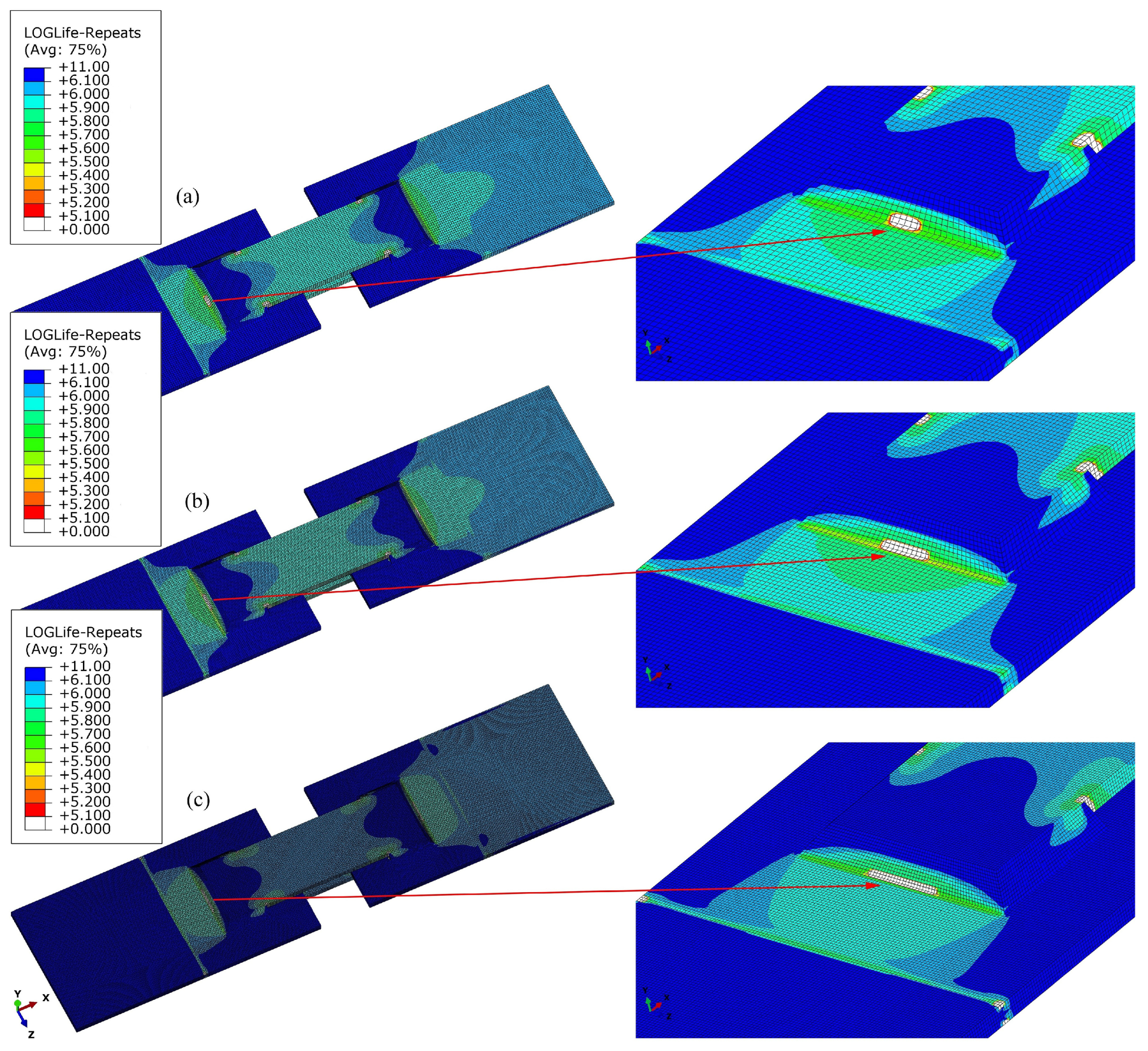
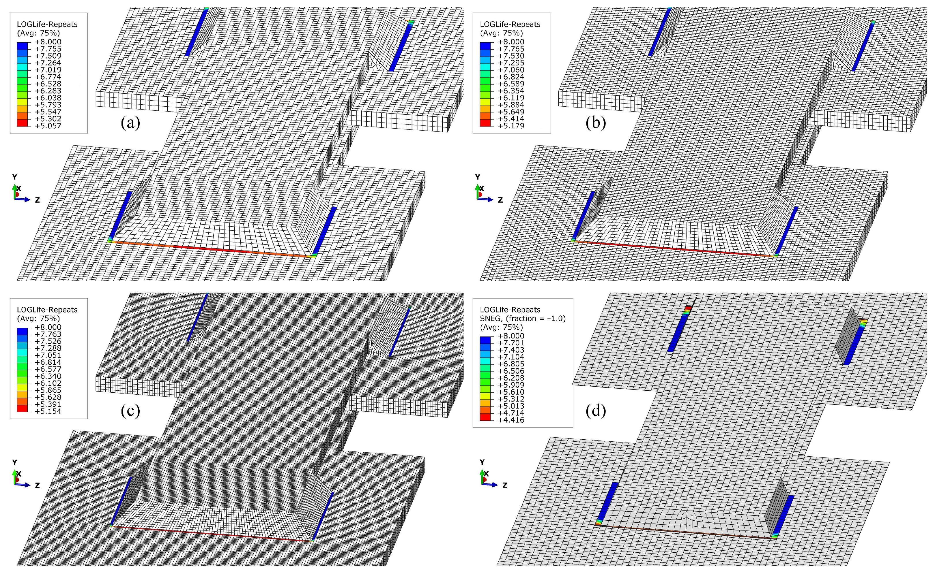
where ${\sigma }_{\mathrm{a}}$, ${\sigma }_{\mathrm{a}0}$, ${\sigma }_{\mathrm{m}}$ and $R_{\mathrm{m}}$ stand for the stress amplitude of the analysed load cycle, the stress amplitude of the analysed load cycle at zero mean stress, the mean stress and the tensile strength of the material, respectively [23]. Fillet welds were defined using the fe-safe/Weld Preparation environment with the stored sets of nodes and elements. Upon the completion of the durability analyses, the predicted number of cycles to failure were obtained in LOGLife format. LOGLife format transforms the number of cycles to failure, N, into the logarithmic form, $logN$, which then enables an easier comparison of small and large numbers.

2.4. Structural Hot-Spot Method

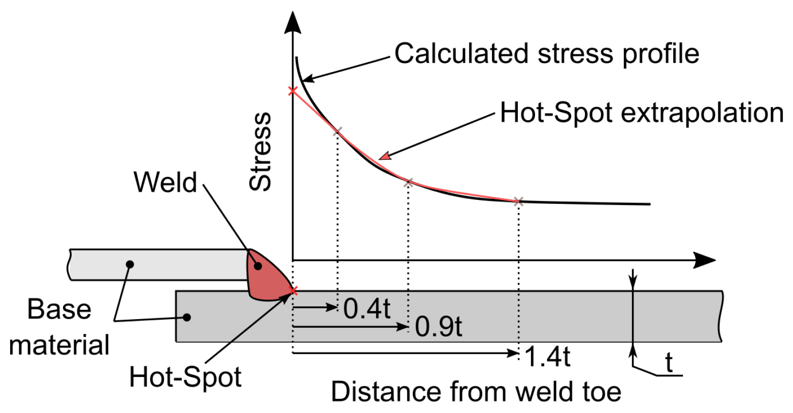
The weakest link in a welded product is the welds. Compared to other means of joining, the welds allow for distributed loading paths and, if executed correctly, a smoother flow of stress compared to, e.g., bolted connection. Welding is an extreme heating and cooling process that in turn disrupts the material lattice of the joined parts. If observed locally, the welds introduce a geometrical feature that acts as a stress concentration detail. This, coupled with diminished mechanical properties of the base material in the heat-affected zone, makes the welds into weak points in the structure. If a welded product is subjected to complex loading and/or is made of complex geometry, an FE method is employed to gain insight into the stress–strain response of the structure. A direct model of the weld would include sharp notches, zero radius transitions and large gradients in the thickness of the material. All these geometrical features are impossible to capture with FEM as they introduce singularity points where no meaningful insights can be gained. 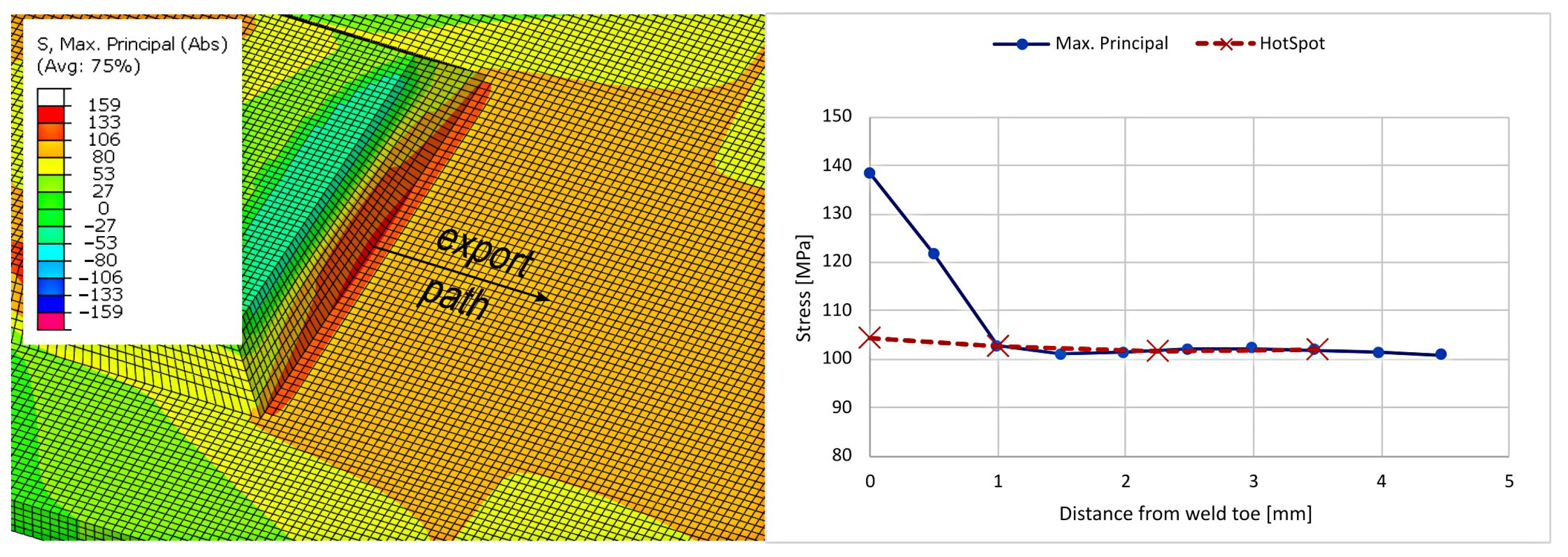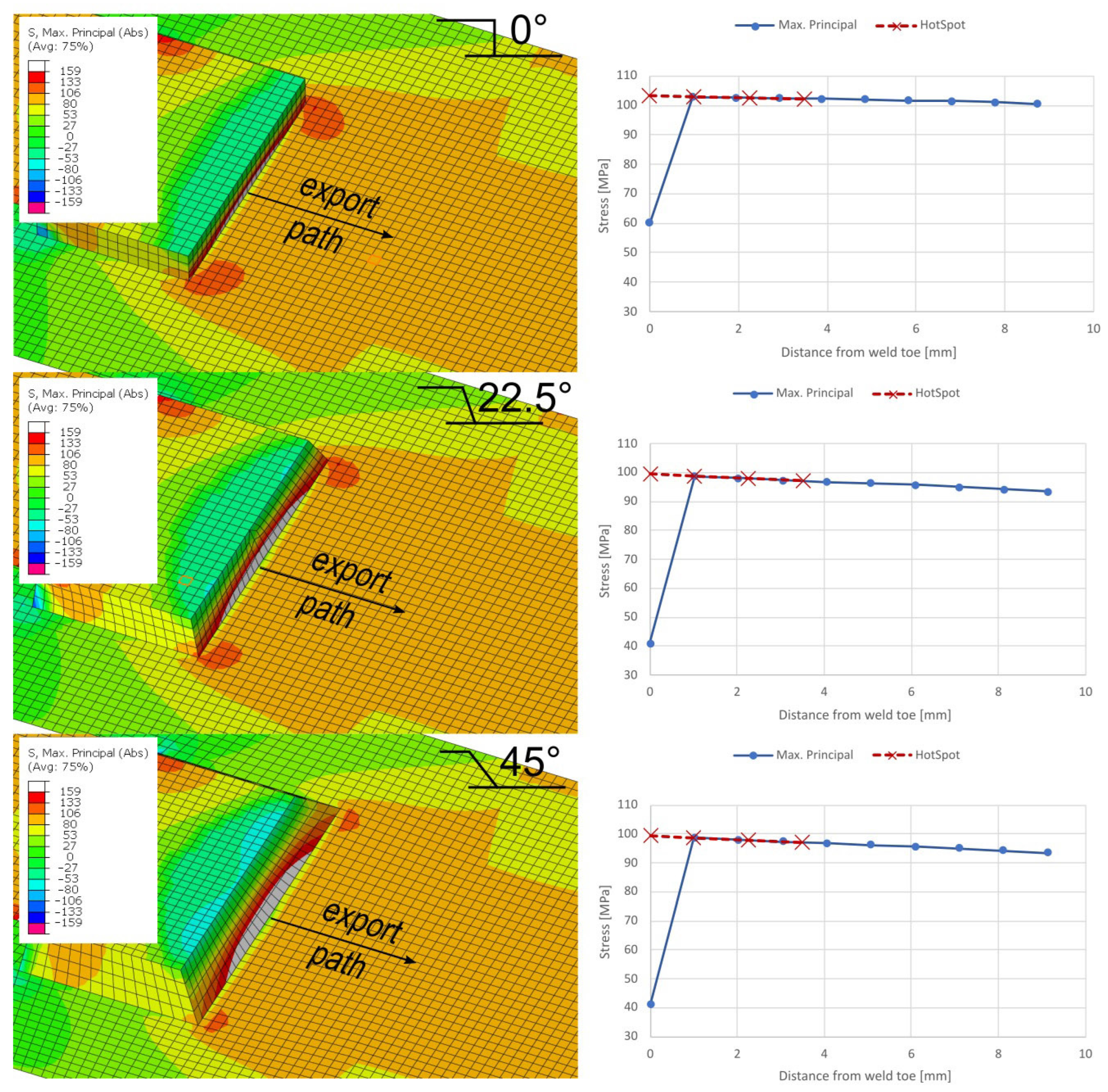A special method termed the Hot-Spot method (HSM) [24] was therefore developed to address this problem. The idea is based on moving the scope of interest away from singularity points. Stresses or strains are observed on a line perpendicular to the weld and are then exported at fractions of material thickness (t) away from the weld toe (Figure 7).

The exported results are now used in a function that extrapolates the so-called Hot-Spot stress in the weld. The extrapolation is based on previous points perpendicular to the welding line at points of maximum computed stress. Moreover, it depends on the stress gradient and FE mesh parameters. In this study, a quadratic extrapolation is applied [24] as

$${\sigma }_{\mathrm{hs}}=2.52·{\sigma }_{0.4·\mathrm{t}}-2.24·{\sigma }_{0.9·\mathrm{t}}+0.72·{\sigma }_{1.4·\mathrm{t}}.$$

(4)

Here, ${\sigma }_{\mathrm{hs}}$ denotes the stress in the Hot Spot, and ${\sigma }_{x·\mathrm{t}}$ is the surface stress along the points at the x factor of t thickness of the material (Figure 7). In this study, the thickness of the material is the nominal $2.5\mathrm{mm}$. The method is suitable for sheet metals, and as we are dealing with fatigue loading, ${\sigma }_{\mathrm{hs}}$ has to be calculated at multiple points in order to access stress range $\mathrm{\Delta }{\sigma }_{\mathrm{hs}}$ in Equation (5),

$$\mathrm{\Delta }{\sigma }_{\mathrm{hs}}=max\left({\sigma }_{\mathrm{hs}}\right)-min\left({\sigma }_{\mathrm{hs}}\right).$$

(5)

The procedure of calculating fatigue life of the weld continues by selecting the appropriate geometric detail. Here, a lap joint is studied which is composed of two fillet welds as shown in Figure 4. The fatigue strength of such a joint is $\mathrm{\Delta }{\sigma }_{\mathrm{hs},\mathrm{ref}}=90\mathrm{MPa}$ at $2\times {10}^6$ load cycles [9]. Unless otherwise specified, the slope of the log(S)–log(N) curve is considered as $m=3$. To calculate the fatigue life at the Hot Spot, Equation (6) has to be solved,

$${\sigma }_{\mathrm{hs}}^m·N_{\mathrm{hs}}={\sigma }_{\mathrm{hs},\mathrm{ref}}^m·2\times {10}^6.$$

(6)

Here, $N_{\mathrm{hs}}$ represents the fatigue life at the Hot Spot which was sought for during this study.

3. Results and Discussion

Simulation results are first separately shown for the use of a fe-safe Verity module and then for the Hot-Spot method. Finally, both results are compared and discussed.

3.1. Simulation Results with FE-Safe Verity

Figure 8a shows the result of the structural analysis using the FE method and the 3D model. Greater stress peaks can be observed locally at the beginning of the welds, which is partly the consequence of the sharp edges of the elements at the end of the geometry. As physical welds can differ from the ideal geometry used in simulations depending on the course, speed and method of welding, rounded edges are usually expected in reality. However, sharper edges can also be observed if the welds are not optimally melted at the start or the end of the welding process. This then proves to be more dangerous as fatigue failures progress faster. The other critical areas in simulations with high stresses appear behind the transverse welds. After the stress concentration of around 140 MPa behind the welds, the stresses decrease into the centre of the clamped sheet metal. Similar results are observed using the 2D FE mesh but with an important difference of higher-stress gradients around the transverse weld (Figure 8b). Experimental failures of the specimens are observed at this location, too (Figure 2).

Based on stress results of structural FE analyses, numerical calculations of durability are performed using fe-safe Verity. In Figure 9, the lifetime predictions are shown if only 3D welds or only 2D welds, respectively, are considered for analysis. Moreover, Figure 9a–c show the calculation for the same geometry of the specimen yet for different densities of FE mesh. The critical areas in the welds are transitions from the slopes of the welds to the central plates regardless of mesh density. The most critical point, however, is in the central longitudinal axis of the specimen of the transverse fillet weld. The intermediate 3D FE mesh density (Figure 9b) resulted in the least conservative durability prediction of the weld (around 150,000 cycles). The results using the 2D mesh, the coarse and the fine 3D meshes are given in

Table 2. Comparison of the durability results using fe-safe Verity with experimental result at load $F_{\mathrm{a}}$ = 11 kN.

Duration— Experimental N (cycles)	Location Max Damage Experimental	Mesh Density	Duration— Fe-Safe Verity N (cycles)	Location Max Damage Simulation
	at	3D rough	114,025 (5.057)	at
159,298	transverse	3D medium	151,008 (5.179)	transverse
	weld	3D fine	142,561 (5.154)	weld
		2D	26,062 (4.416)

The results in brackets are given in LOGLife format—see Figure 9.

.

Performing a durability analysis in fe-safe Verity, both the welds and the surrounding material (sheet metals) can simultaneously be considered, too (Figure 10). Here, all the settings remain the same as in the previous analysis for 3D welds only, but this time the geometry of the sheets is also included in calculation. The critical point in this case remains the transverse fillet weld (if the beginnings and ends of the welds are excluded), which is the same location of fatigue damage/failure as observed during physical tests (Figure 2 above). The estimated lifetime until the formation of an initial crack or damage is calculated as 130,000 cycles and is comparable to that of the previous weld-only analysis. Some differences can be noticed in the form of critical area, i.e., a more oval area using the coarse FE mesh and a stretched and thin area using the fine mesh. Fatigue design using the fe-safe module is an approach used to prevent the initiation of cracks. For many engineering components, this represents the total design life. The calculated durability is hence the number of cycles to crack initiation. For high-cycle fatigue, the experimental determination of the durability also mostly comprises the crack initiation stage. A study of Klemenc and Nagode [25] showed that the crack in CP-W800 in high-cycle fatigue consisted of 98.5% of crack initiation stage and 1.5% of crack propagation stage. Nevertheless, for higher loads, the ratio between the two stages changes, so both the simulations and the experimental determination of the durability should consider the change in the damage mechanism.

3.2. Simulation Results with Hot-Spot Method

Abaqus was also used first to gain the surface Hot-Spot stresses on the 3D model of the welded specimen. Both 3D and 2D FE meshes were used to export the results. The results of the 3D mesh are shown in Figure 11. The displayed result shows the maximum principal stress magnitude at full tension of a fully reversed ($R=-1$) study. Due to the symmetry of the loading conditions, the results in compression differ marginally in magnitude. FE elements of type C3D8 were used with a global size of $0.5\mathrm{mm}$. Using the 2D mesh, the surfaces at weld locations were joined at different angles as displayed in Figure 12. All the surfaces, base material and weld, were assigned five section integration points and a thickness of 2.5 mm. FE elements of type S4 were used with a global size of $1\mathrm{mm}$. The results of durability calculation using the Hot-Spot method according to Equations (4)–(6) are given in

Table 3. Durability calculation results based on the Hot-Spot method.

Mesh	${\mathit{\sigma }}_{\mathbf{hs}}$	$\mathbf{\Delta }{\mathit{\sigma }}_{\mathbf{hs}}$	Predicted Number of Cycles to Failure
3D	104	208	160,540
2D 0°	103	206	165,562
2D 22.5°	99	198	185,456
2D 45°	95	190	207,290

.

3.3. Comparison of Results

The difference in durability prediction using the fe-safe Verity module is associated with the gap between the sheet metals, which was meshed by one layer of finite elements that could differ depending on the global size of the mesh. The coarser mesh could therefore represent a somewhat stiffer structure in this area, which then resulted in a more conservative durability prediction. Nevertheless, durability predictions were always more conservative than the experimental result (around 160,000 cycles). This was expected as the stress-based approach for durability was used which traditionally provides more conservative predictions. The predicted number of cycles was especially conservative in the case of the 2D mesh, which could again be attributed to the immense and sudden change in stress around the transverse weld (Figure 9d and Table 2).

Durability predictions using either the fe-safe Verity module or the Hot-Spot method proved comparable in this study if a 3D FE mesh was used. Predictions using fe-safe Verity were marginally conservative, whereas the application of the Hot-Spot method resulted in slightly non-conservative predictions. Here, it has to be mentioned that not insignificant scatter was also observed during experimental testing of durability (Figure 3). Considering this, a more appreciable comprehension of the prediction can be drawn. The main reason for such results can most clearly be explained if the Hot-Spot results for 2D FE are observed. They exhibit a peculiar trend near the weld toe; a sudden drop of stress is noticed. The results in Figure 12 depict the results from the integration points that represent the model surface. As the Hot-Spot method focuses on points away from the weld toe, the initial stress point does not affect calculation. In comparison with 3D results, 2D simplification therefore yields a less intense stress state near the weld. This then affects the durability calculation presented in Table 3.

The physical shape of the weld is rarely the same as the idealised geometric form provided in the technical documentation and used in predictions. However, it is an engineering reality which is then manifested in the scatter of the experimental results under equal loading conditions. This influence is therefore already considered in the durability curves and the methods used to calculate durability. Specifically due to this phenomenon, the structural Hot-Spot method utilises the stresses in the sheet metal rather than the stress in the weld to predict the durability of the welds. Although the stress distribution in the weld might be affected, this influence is reduced in sheet metal.

4. Conclusions

The study compared durability predictions of fillet welds based on two methods of structural stresses. Durability predictions using the fe-safe Verity method proved somewhat conservative and comparable to the experimental results of the durability of the welds on the specimen. The main advantage of the method is its small sensitivity to mesh density, which proved correct for the 3D FE mesh. As high stress concentration appeared around the weld in the case of the 2D FE mesh, a more conservative durability prediction was hence observed. A comparable prediction to a fe-safe Verity module was obtained using the Hot-Spot method in the case of the 3D FE mesh. On the contrary, a less conservative durability prediction was observed with the Hot-Spot method in the case of the 2D FE mesh as the stress concentration influence was reduced in the area which is considered for extrapolation of the stress state in the welds.

References

1. Zheng, J.; Ince, A.; Tang, L. Modeling and simulation of weld residual stresses and ultrasonic impact treatment of welded joints. Procedia Eng. 2018, 213, 36–47. [Google Scholar] [CrossRef]
2. Khoshnaw, F.; Krivtsun, I.; Korzhyk, V. Arc welding methods. In Welding of Metallic Materials; Elsevier: Amsterdam, The Netherlands, 2023; pp. 37–71. [Google Scholar] [CrossRef]
3. Swapna Sai, M.; Dhinakaran, V.; Manoj Kumar, K.P.; Rajkumar, V.; Stalin, B.; Sathish, T. A systematic review of effect of different welding process on mechanical properties of grade 5 titanium alloy. Mater. Today Proc. 2020, 21, 948–953. [Google Scholar] [CrossRef]
4. Chiocca, A.; Frendo, F.; Aiello, F.; Bertini, L. Influence of residual stresses on the fatigue life of welded joints. Numerical simulation and experimental tests. Int. J. Fatigue 2022, 162, 106901. [Google Scholar] [CrossRef]
5. Łagoda, T.; Głowacka, K. Fatigue life prediction of welded joints from nominal system to fracture mechanics. Int. J. Fatigue 2020, 137, 105647. [Google Scholar] [CrossRef]
6. Ottersböck, M.J.; Leitner, M.; Stoschka, M. Characterisation of actual weld geometry and stress concentration of butt welds exhibiting local undercuts. Eng. Struct. 2021, 240, 112266. [Google Scholar] [CrossRef]
7. Vemanaboina, H.; Akella, S.; Buddu, R.K. Welding Process Simulation Model for Temperature and Residual Stress Analysis. Procedia Mater. Sci. 2014, 6, 1539–1546. [Google Scholar] [CrossRef]
8. DIN 15 018-1; Cranes; Steel Structures; Verification and Analyses. Beuth Verlag: Berlin, Germany, 1984.
9. EN 1993-1-8:2005; Eurocode 3: Design of Steel Structures—Part 1–8: Design of Joints. CEN: Brussels, Belgium, 2005.
10. ASTM Standards for Welding, 4th ed.; ASTM: West Conshohocken, PA, USA, 2020.
11. Hobbacher, A.F. The new IIW recommendations for fatigue assessment of welded joints and components—A comprehensive code recently updated. Int. J. Fatigue 2009, 31, 50–58. [Google Scholar] [CrossRef]
12. Lee, J.M.; Seo, J.K.; Kim, M.H.; Shin, S.B.; Han, M.S.; Park, J.S.; Mahendran, M. Comparison of hot spot stress evaluation methods for welded structures. Int. J. Nav. Archit. Ocean. Eng. 2010, 2, 200–210. [Google Scholar] [CrossRef]
13. Al Zamzami, I.; Susmel, L. On the use of hot-spot stresses, effective notch stresses and the Point Method to estimate lifetime of inclined welds subjected to uniaxial fatigue loading. Int. J. Fatigue 2018, 117, 432–449. [Google Scholar] [CrossRef]
14. Maddox, S.J. Recommended Hot-Spot Stress Design S-N Curves For Fatigue Assessment of FPSOs. In Proceedings of the Eleventh International Offshore and Polar Engineering Conference, Stavanger, Norway, 17–22 June 2001; p. ISOPE–I–01–354. [Google Scholar]
15. Karabulut, B.; Rossi, B. On the applicability of the hot spot stress method to high strength duplex and carbon steel welded details. Eng. Fail. Anal. 2021, 128, 105629. [Google Scholar] [CrossRef]
16. He, Z.; Chen, B.; Li, X. Comparative study on numerical simulation methods of stress concentration calculation and fatigue life prediction for welds. Int. J. Fatigue 2023, 166, 107205. [Google Scholar] [CrossRef]
17. Dong, P. A structural stress definition and numerical implementation for fatigue analysis of welded joints. Int. J. Fatigue 2001, 23, 865–876. [Google Scholar] [CrossRef]
18. Dong, P.; Hong, J.; Osage, D.A.; Prager, M. Master S-N Curve Method for Fatigue Evaluation of Welded Components; Welding Research Council Bulletin: Shaker Heights, OH, USA, 2002; Volume 474. [Google Scholar]
19. Alencar, G.; Hong, J.K.; de Jesus, A.; da Silva, J.G.S.; Calçada, R. The Master S-N curve approach for fatigue assessment of welded bridge structural details. Int. J. Fatigue 2021, 152, 106432. [Google Scholar] [CrossRef]
20. Selvakumar, P.; Hong, J.K. Robust mesh insensitive structural stress method for fatigue analysis of welded structures. Procedia Eng. 2013, 55, 374–379. [Google Scholar] [CrossRef]
21. FeSafe Module VERITY. Available online: https://www.3ds.com/products/simulia/fe-safe/verity-module (accessed on 30 August 2023).
22. Muc, M. Estimating Durability of Dynamically Loaded Weld Joints. Master’s Thesis, University of Ljubljana, Faculty of Mechanical Engineering, Ljubljana, Slovenia, 2018. [Google Scholar]
23. Dassault Systemes. FE-Safe 2021; Dassault Systemes Simulia Corp: Velizy-Villacoublay Cedex, France, 2020; Volume 1. [Google Scholar]
24. Hobbacher, A. Recommendations for Fatigue Design of Welded Joints and Components; Springer: Berlin/Heidelberg, Germany, 2016; Volume 47. [Google Scholar]
25. Klemenc, J.; Nagode, M. Design of step-stress accelerated life tests for estimating the fatigue reliability of structural components based on a finite-element approach. Fatigue Fract. Eng. Mater. Struct. 2021, 44, 1562–1582. [Google Scholar] [CrossRef]
Figure 1. The geometry of the welds on the joint of the tested sheet metal.
Solids 05 00006 g001
Figure 2. A ruptured specimen of CP-W800 steel (above) tested on an electro-mechanical test rig SCHENCK (below).
Solids 05 00006 g002
Figure 3. Wöhler curves for CP-W800 steel at different failure probabilities, retrieved from [22].
Solids 05 00006 g003
Figure 4. (a) Importing a single geometry into Abaqus (initial part), (b) dividing a single geometry into sections (partitions) to build a structured FE mesh and (c) defining the supports (right) and the load (left) of the specimen.
Solids 05 00006 g004
Figure 5. Different 3D mesh densities: (a) the coarsest, (b) intermediate and (c) the finest structured FE mesh.
Solids 05 00006 g005
Figure 6. Marking of (a) nodes and (b) elements to identify the welds.
Solids 05 00006 g006
Figure 7. Principle of Hot-Spot stress determination (created after [24]).
Solids 05 00006 g007
Figure 8. Stress results (MPa) using (a) 3D and (b) 2D FE mesh of the specimen.
Solids 05 00006 g008
Figure 9. Evaluation of the durability of fillet welds, for the cases of (a) coarse, (b) medium and (c) fine 3D FE mesh and (d) 2D FE mesh.
Solids 05 00006 g009
Figure 10. Estimated lifetime: combined effect of welds and surrounding sheets, for (a) coarse, (b) medium and (c) fine 3D FE mesh.
Solids 05 00006 g010
Figure 11. (left) Maximum principle stress state for 3D FE mesh and (right) comparison of the stress state along the exported path and the Hot-Spot method extraction of stress.
Solids 05 00006 g011
Figure 12. (left) Maximum principle stress state for 2D FE mesh and (right) comparison of the stress state along the exported path and the Hot-Spot method extraction of stress.
Solids 05 00006 g012