Sub-Surface Soil Characterization Using Image Analysis: Material Recognition Using the Grey Level Co-Occurrence Matrix Applied to a Video-CPT-Cone

Abstract

The geotechnical characterization of the subsurface is a key requirement for most soil investigations, incl. those for reclaiming landfills and waste dumps associated with mining operations. New sensor technology, combined with intelligent analysis algorithms, allow for a faster and less expensive acquisition of the necessary information without loss of data quality. The use of advanced technologies to support and back up common site investigation techniques, such as cone penetration testing (CPT), can enhance the underground characterization process. This study aims to investigate the possibilities of image analysis for material recognition to advance the geotechnical characterization process. The grey level co-occurrence matrix (GLCM) image processing technique is used in a wide range of study fields to estimate textures, patterns and structure anomalies. This method was adjusted and applied to process the video recorded during a CPT sounding, in order to distinguish soil types by its changing surface characteristics. From the results of the video processing, it is evident that the GLCM technique can identify transitions in soil types that were captured in the video recording. This enables the prospect of image analysis not just for soil investigations, but also for monitoring of the conveyor belt in the mining field, to allow for efficient preliminary decision making, material documentation and quality control by providing information in a cost effective and efficient manner.

1. Introduction

Across the entire lifespan of a mine, spanning from exploration and production to closure, the implementation of automated processes for recognizing and characterising materials, without compromising the information quality, can significantly enhance value [1]. It streamlines the analysis, reduces associated costs, and opens up opportunities to expedite decision-making on various aspects, such as estimation of material type and quality, future planning, assessment of ongoing processes, validation of waste dump models and evaluation of geotechnical site investigations in general [2]. Furthermore, it establishes a comprehensive spatio-temporal database that complements the limited and costly data obtained through physical sampling and laboratory analysis [3].

One of the notable features that affects the decision-making process during any mining stage is the subsurface profile, both with respect to material type and material properties. During the planning phase a thorough understanding of the subsurface is required to plan the location of the tailings storage facilities. And when it comes to the transformation of an area once the mining operations are ended, to assess the safe and environmentally friendly options for a post-mining landscape, the heterogeneous subsurface (incl. that of landfills and waste dumps) has to be characterized in terms of geotechnical parameters. These parameters are affected by the subsurface material types and textures [4,5,6]. Moreover, soil type and texture define properties, such as permeability [7], liquefaction potential [8], and freezing properties [9] that affect choice of material handling machines required to construct the planned facility or landscape.

There are numerous in situ site investigation techniques (which include cone penetration testing [10,11]) and laboratory testing to determine all kinds of soil parameters. Considering that these techniques are expensive and time consuming, any method to quickly obtain preliminary or additional information on material properties provides an advantage. That is where optical sensors and computer vision come into play as non-invasive material analysis methods. One type of computer vision that provides numerous possibilities for material recognition is image analysis. It offers a wide range of techniques that suit various needs of multiple study fields. Many of these techniques can be used to characterise features that can be correlated to the behaviour and stress-related deformability of soils such as the grain-size distribution, compressibility, etc. [12].

Already long-established image processing techniques, such as the grey level co-occurrence matrix (GLCM), are used to estimate textures, patterns and structure anomalies in a wide range of fields, from the medical field (identification cancer tissues [13,14], bone fractures [15]; etc.) to geography [16,17] and mining [18,19,20].

This article aims to test the image-based material recognition in soil material streams using the grey level co-occurrence matrix. Results of this could possibly enhance the process of any site investigation, including those for the post-mining landscape transition, and thus improve the decision making. Compared to commonly used techniques, such as laboratory testing, it has a potential time and cost advantage without diminishing the evaluation precision. This contribution discusses an innovative application of the GLCM to complementary support CPT data.

GLCM correlation and dissimilarity parameters, the calculations of which are discussed in the methodology chapter of this article, were chosen as the most appropriate for the precognition and characterization of the soil material due to the clear material thresholds that were computed. The cone penetration test approach is also described in said chapter and used for the image analysis validation.

The input data for the current study is the video recorded during the CPT sounding. Its set up, material and input description are included in the “Application set-up” chapter.

In conclusion, the image processing technique, discussed in this paper, proved to be efficient at recognising the soil behaviour type during a routine CPT sounding in a Tailings Storage Facility. A similar approach and set up can be adapted for various other mining purposes, such as video monitoring of conveyor belts for documentation of material within the dump.

2. Materials and Methods

2.1. Image Processing for Soil Texture Recognition

Image processing contains a versatile set of techniques that offers a diverse range of requirements in the scope of image manipulation and feature extraction. These methods provide extensive capabilities, allowing for the enhancement, modification, and analysis of images, as well as the extraction of relevant features for various applications.

An image comprises two essential components. The initial element involves the intensities of light waves reflected from the smallest addressable unit of the image, known as a pixel. Pixels serve as the fundamental encoding units for all digital images. In standard digital images representing colour, three specific wavelengths (or bands) are typically recorded. In contrast to hyperspectral or multispectral images, which may have up to 1000 registered bands, digital images offer simplicity in representation and ease of comprehension, making them compatible with most modern devices and displays. The combination of pixel bands creates the perceived colours in our brains. The second crucial component for image analysis is the spatial configuration. Each image fundamentally forms a matrix of pixels, each occupying a specific position and having coordinates. Many image analysis techniques rely on calculating statistical relationships between neighbouring pixels and establishing the “distance” over which these calculations are performed [21,22].

Depending on the analysis goal, the techniques will concentrate around either processing the dependencies between the pixels that create the image or calculating the characteristics of the objects within the image. This divides the image analysis field into two major parts: pixel-based methods and object-based methods.

Pixel-based methods focus on analysis of the image colour parameter. These methods determine the correlation between pixel intensities, amount of colour groups, regularity and homogeneity of image overall. Pixel-based methods include techniques such as thresholding and k-mean segmentation, which group pixels by its colour features, as well statistical methods (grey level co-occurrence matrix—GLCM), structural methods, model-based (fractal models) methods, and transform-based methods for recognizing image textures and patterns [23]. All these methods have their own advantages and disadvantages, as well as practicality, depending on image complexity and analysis objective. For example, in cases when the matter of image components should be detected and estimated and computation of exact components edges is not possible (e.g., mineral veins in the rock material), separating those elements by colour groups is a convenient approach.

Object-based approaches are used to segment the image elements, by grouping pixels into vector objects, and their spectral, geometrical, and spatial properties are used to further derive the features out of them [24]. In contrast to the pixel-based approaches that concentrate on the image of the smallest elements that are the same shape and form, and analysing each of them, object-based techniques focus on the analysis of separately created regions.

In the study case described in this article, in order to quickly recognize soil layers when the video sample is displaying movement through these layers, the analysis of the image patterns leads to the choice of statistical texture analysis, in particular grey level co-occurrence matrix, which offers a fairly simple and fast way to process an image, separate its elements, and recognize textures as well as patterns.

2.2. The GLCM

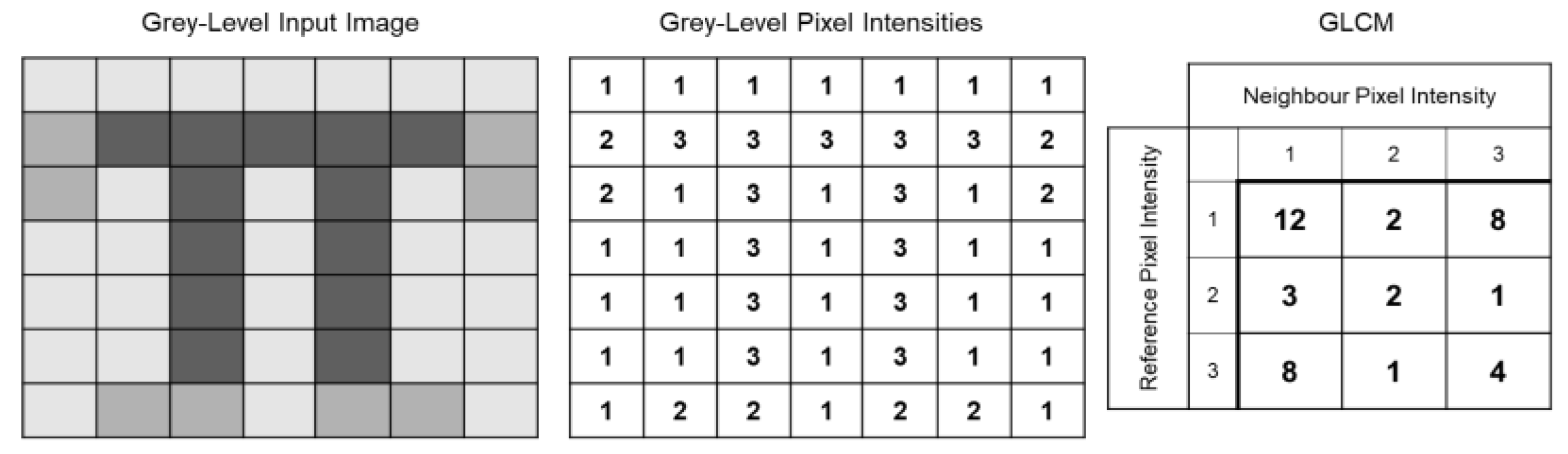
The grey level co-occurrence matrix (GLCM) is a statistical method for deriving texture features considering the relationship between groups of two pixels in the image at a certain distance and at a certain angle. The GLCM is a square matrix of order N, where the (i, j) entry represents the number of occasions a pixel with intensity i is adjacent to and a pixel with intensity j and N is the number of intensities considered. Distance parameters can range from 1 pixel to the image size, while the typical direction angles between pixels are 0°, 45°, 90° and 135°. The direction choice is important for pattern recognition and should be considered carefully. As soil material patterns are generally invariant to rotation, extracted textural features can be averaged over all four main angle inputs [25].

In order to construct the GLCM with its elements (Pi,j), the number of times when a pair of pixels with grey levels i and j appear next to each other is recorded. An example is provided in Figure 1 [26]. The grey level input image (on the left side of Figure 1) consists of three grey levels, 1, 2 and 3. The corresponding intensity coded representation is shown in the middle. The GLCM for a 0° direction and a distance of one pixel is shown on the left side of the figure.

Texture value calculations use the weighted averages of the normalised grey level co-occurrence matrix. These weights express relative significance of the value. Texture measures can be grouped by descriptive statistics and by contrast class that weighs distance to the GLCM diagonal.

2.2.1. GLCM Correlation

GLCM correlation are descriptive statistics of GLCM that measure grey levels’ linear dependencies of neighbouring pixels on an image and is expressed as follows:

$$Cor(i,j)=\sum _{i,j=0}^{N-1}{P}_{i,j}\left[\frac{(i-{\mu }_i)(i-{\mu }_j)}{\sqrt{\left({\sigma }_i^2\right)\left({\sigma }_j^2\right)}}\right]$$

(1)

where $P_{i,j}$ is element at row i and column j of the normalised GLCM, ${\mu }_i$ and ${\mu }_j$are mean values of GLCM and ${\sigma }_i^2$, ${\sigma }_j^2$ their variances [27].

GLCM mean values are pixel values weighed by frequency occurrence in relation to a neighbour pixel value (Equations (2) and (3)) and GLCM variance is dependent on the mean to determine the dispersion around it in reference to the neighbour pixel (Equations (4) and (5)).

$${\mu }_i=\sum _{i,j=0}^{N-1}i\left(P_{i,j}\right)$$

(2)

$${\mu }_j=\sum _{i,j=0}^{N-1}j\left(P_{i,j}\right)$$

(3)

$${\sigma }_i^2={\sum }_{i,j=0}^{N-1}{P}_{i,j}{(i-{\mu }_i)}^2,$$

(4)

$${\sigma }_i^2={\sum }_{i,j=0}^{N-1}{P}_{i,j}{(i-{\mu }_i)}^2,$$

(5)

The GLCM correlation between neighbouring pixels indicates their predictable and linear relationship and ranges from −1 to 1: a correlation with value −1 is considered negatively correlated, value 0 signifies uncorrelated, while a value of 1 is positively correlated [28].

2.2.2. GLCM Dissimilarity

GLCM dissimilarity is one of the contrast measures of texture features and is given as follows:

$$Dissimilarity(i,j)={\sum }_{i,j=0}^{N-1}{P}_{i,j}\left|i-j\right|,$$

(6)

When i and j are equal, the matrix cell is located on the diagonal. Therefore, the two pixels are similar, the given weight is 0 and there is no contrast. As the difference between pixel pairs increases, the weight increases linearly [29].

Differences in values of the GLCM described above for features of specific elements on the input image or the image overall can indicate differences in recorded materials.

The GLCM dissimilarity and correlation features, along with their respective parameters, were identified as the most representative material indicators based on a series of tests. It was observed that certain features, such as GLCM homogeneity and energy, generated nearly identical results and plots to features mentioned before.

2.3. Cone Penetration Test

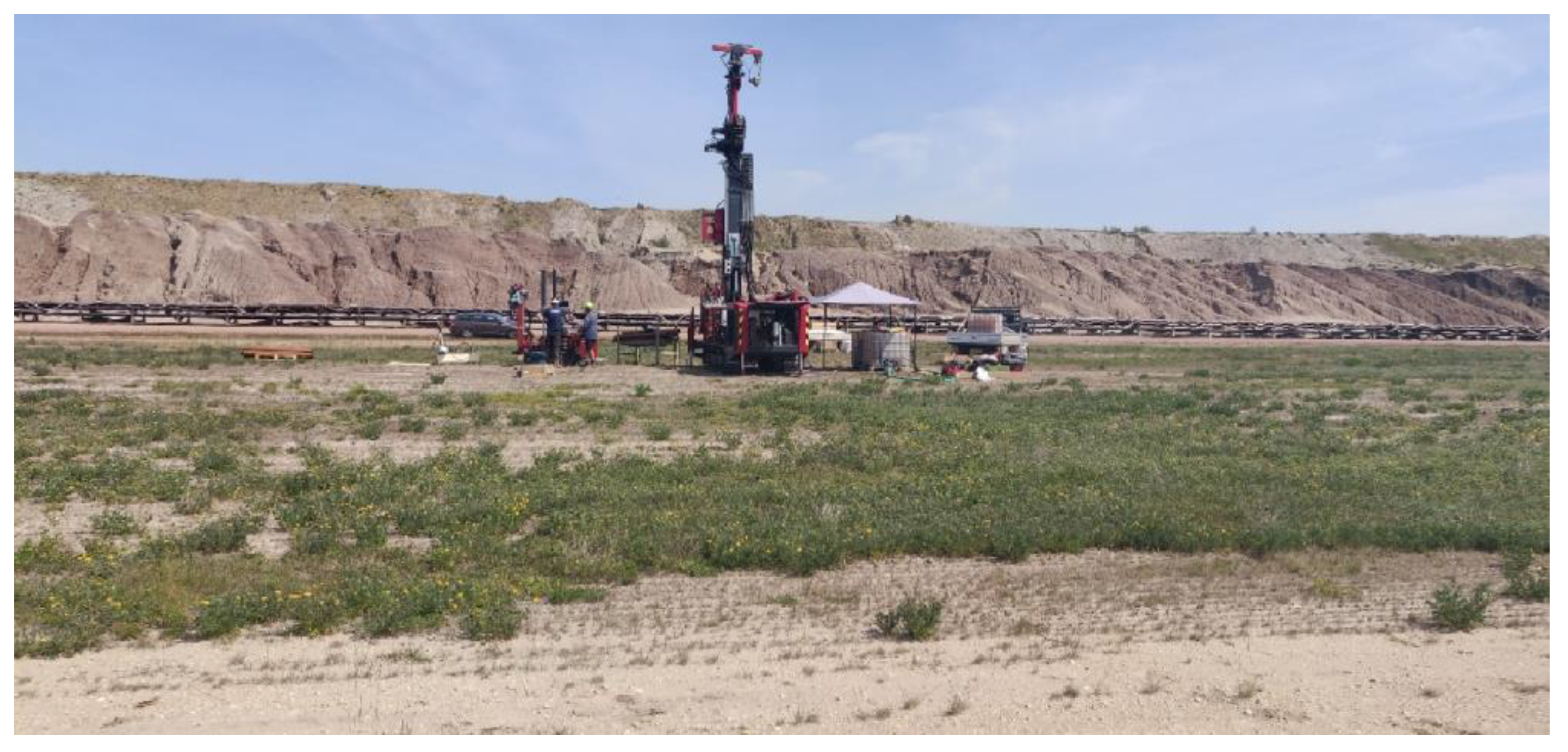
To validate the proposed method, results of material recognition obtained from image analysis were compared to cone penetration test (CPT) data [30] and soil behaviour type plots from the same location. Soil types included tertiary sands, silts and clays from the Leipzig coal basin in Germany (see Figure 2).

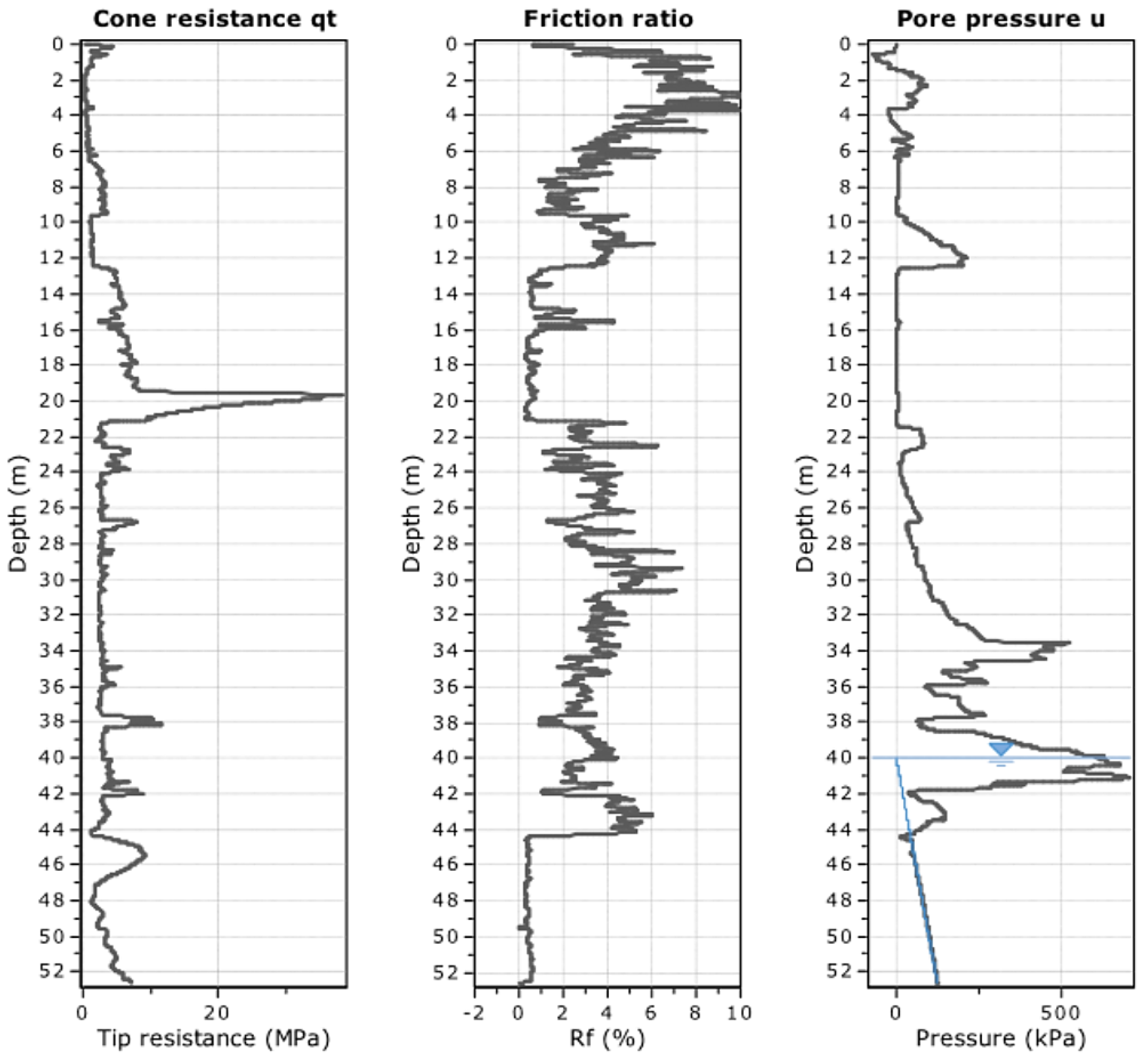
To perform the cone penetration test, a 10 cm² subtraction cone was pushed into the ground at a constant and standardized rate. Simultaneously, the measurement of the ground resistance to the cone tip was measured, by dividing the total force acting on the cone by the projected area of the cone, as well as the friction along the friction sleeve of the cone and the dynamic pore pressure [10,27]. 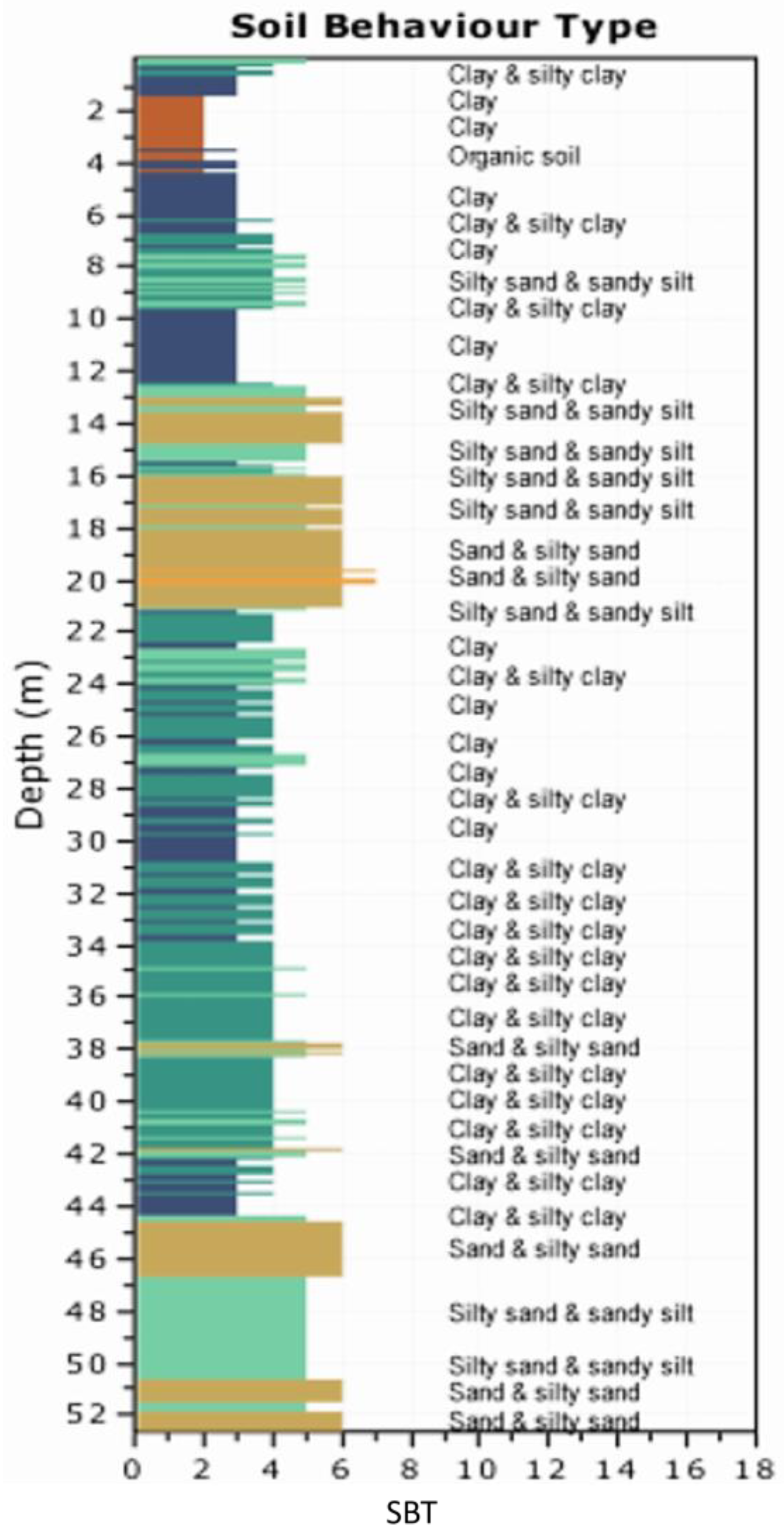These parameters were recorded at 10 mm intervals as the cone penetrated the soil, generating a continuous soil profile (see Figure 3). The data obtained was analysed to derive the soil behaviour type (SBT) using the Robertson—Campanella chart [11], and the results are shown in Figure 4. While the SBT classification does not necessarily correspond to the soil type (since certain soils can behave like a different soil type), in most cases there is a very strong correlation between SBT and soil type. For this test, this was confirmed as additional soil borings were performed that showed that the SBT matched the soil type.

The operation was executed as part of the EU-project “TRIM4Post-Mining” inside a waste dump of a lignite mine operated by MIBRA GmbH, Germany. The cone penetration test (CPT) data showed a distinct soil profile, primarily composed of cohesive soils extending to approximately 44 m, with granular soil beneath it. However, the cohesive layer was interrupted by an intermediate layer of granular soil types between 13 m and 21 m. The dynamic pore pressure curve also indicated the transition to the granular soil type at around 13 m, since it suddenly dropped when the cone was moved from a layer with low hydraulic conductivity (the cohesive soil layer) to one with much higher hydraulic conductivity (the granular soil layer).

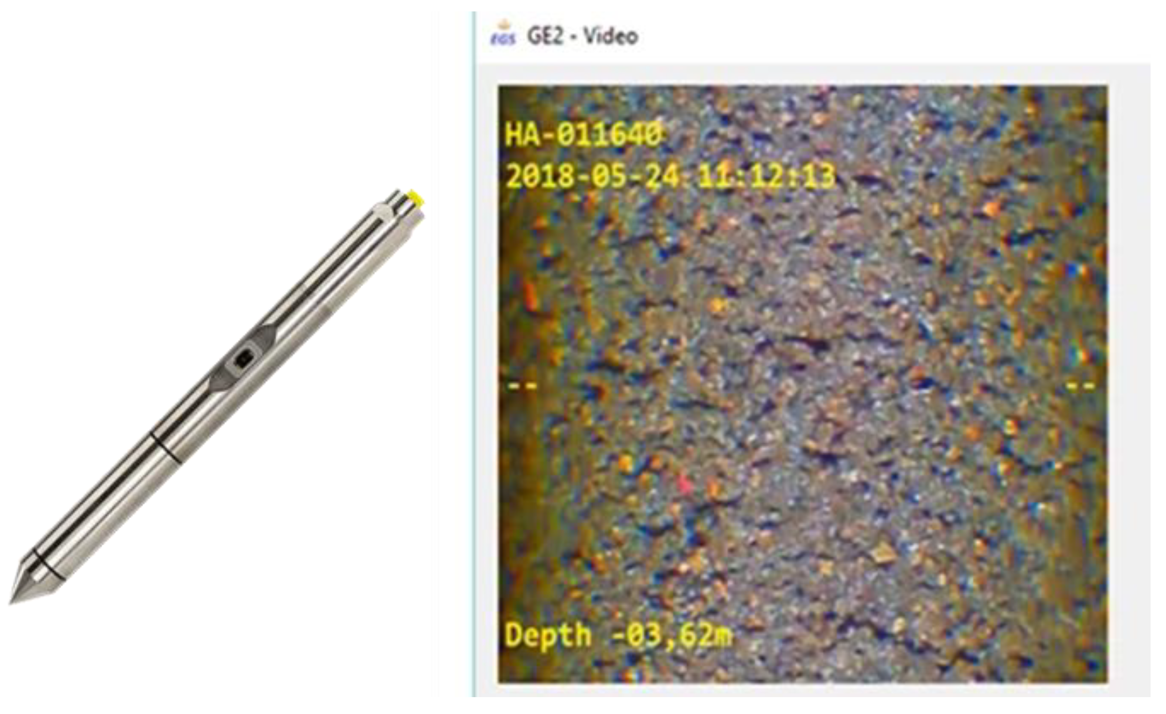
For this test, a module was mounted behind the CPT cone with a miniature colour SD video camera (Figure 5). This camera recorded the soil passing camera lens, as the cone penetrates the soil. The images were then used to test the ability of the image-based texture recognition technique.

2.4. Application Set-Up

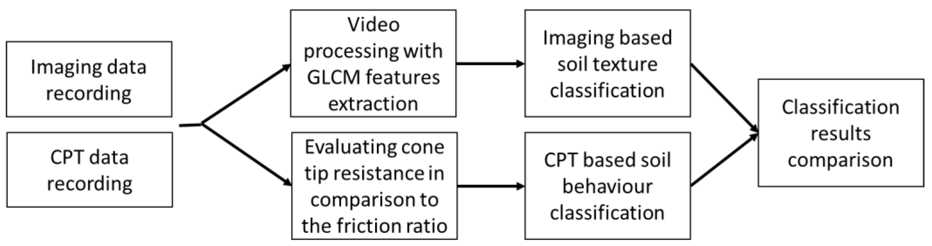
For this research input, verification data (video recordings during the CPT using a small digital camera installed in the cone and the CPT data, respectively) were collected simultaneously during the CPT sounding as shown in the research workflow (Figure 6). This ensures not only functionality of the data collection in an on-site environment, but also benefits the comparison and verification of the study.

To reduce the amount of input data, the algorithm was run over a 13 min video containing the recordings of the video camera between 12 m and 15 m, which includes the distinctive change in soil type mentioned earlier. Overall, the video contains around 19,540 frames.

It is worth mentioning that CPT data is commonly presented in relation to penetration depth, while GLCM texture features are presented against timestamps for each frame. As an example, in this study case covering a depth interval of 3 m, there were 307 CPT data points and 19,540 useable frames. This obviously complicates the computation of quantitative validation of the results, and it is recommended that in future studies the time stamp of each CPT data point is used.

To compare the two derived indexes, one image based and the other CPT-based, the Pearson correlation coefficient was computed, using a reduced dataset on 15 cm depth intervals extracted from the video input and corresponding to the depth of CPT data input. The Pearson correlation coefficient is a statistic that describes the strength and direction of the linear relationship between two quantitative variables [31] and presented as follows:

$$r={\sum }_i^{ }\frac{(x_i-\underset{\_}{x})(y_i-\underset{\_}{y})}{\sqrt{{\sum }_i^{ }{(x_i-\underset{\_}{x})}^2}\sqrt{{\sum }_i^{ }{(y_i-y)}^2}},$$

(7)

where $\underset{\_}{x}$ is the mean of the vector x and $\underset{\_}{y}$ is the mean of the vector y.

In this research, CPT data are used as the x-values, and GLCM data serve as the y-variables for calculating the correlation coefficient.

Pearson correlation coefficient ranges between −1 and 1. Values between 0 and 1 signify positive correlation, where with a change of one variable, the other variable also changes in the same direction. A value of 0 denotes no correlation, whereas values ranging from 0 to −1 signify a negative correlation.

3. Results

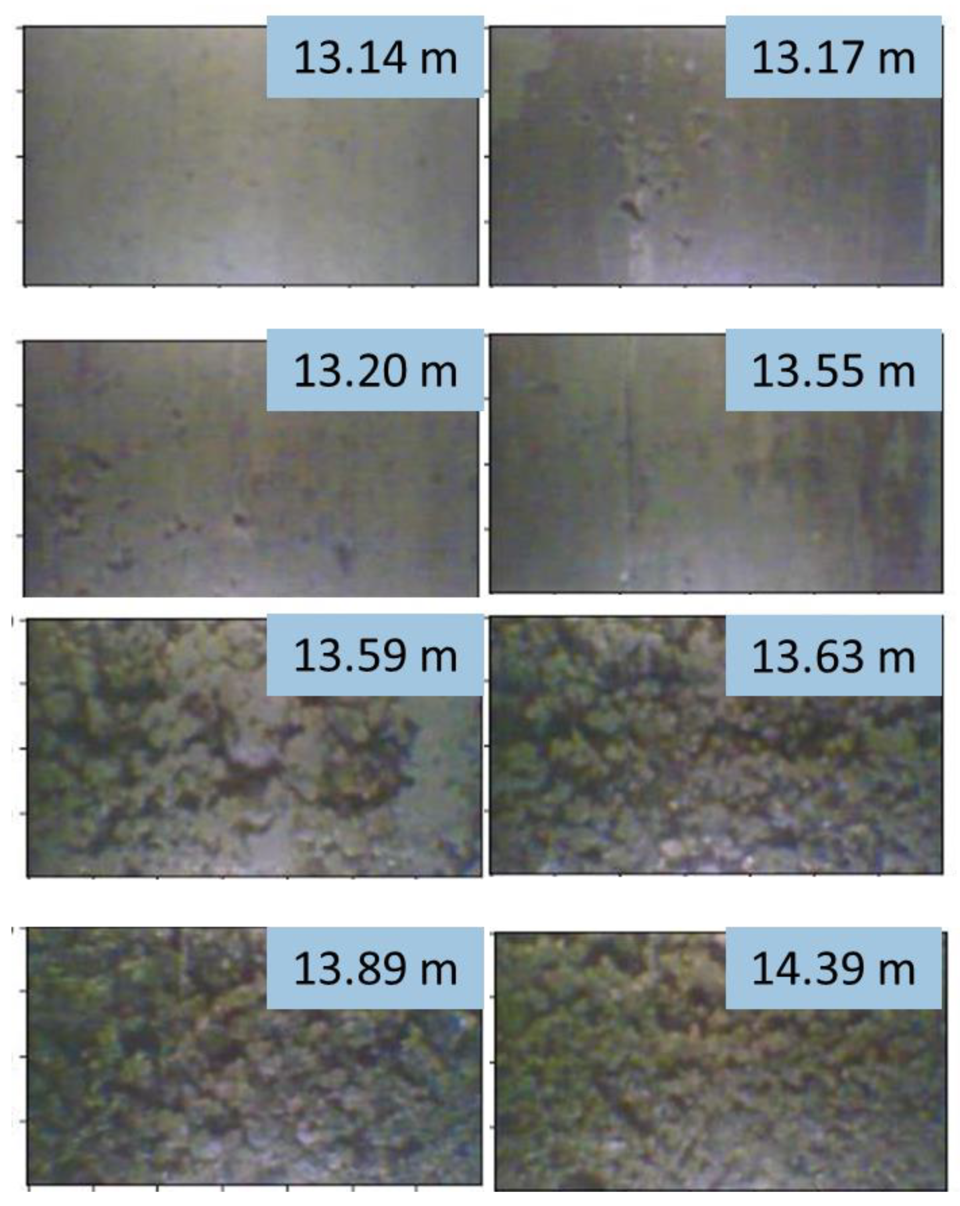
To test the methodology and the possibility of recognising different material textures, first a limited data set was created in the form of eight carefully selected frames from the captured video. Those frames represent clay and sand, respectively (Figure 7).

According to Indian standard nomenclature [32], soils are categorized into four groups based on their particle size:

• gravel—80 mm to 4.75 mm
• sand—4.75 mm to 0.075 mm
• silt—0.075 mm to 0.002 mm
• clay—less than 0.002 mm

This categorization serves as a clue to predict the visual characteristics of soil texture.

The additional goal of this experiment was also to recognize the conditions, during which the result of image and video analysis would be sufficient. These conditions include lighting, camera resolution and the presence of material movement against the camera from its pressure and water presence.

To address the lighting conditions, the extra enhancement filter was applied on these images. This corrected the slight shadowing on the frame edges without distortion of the original image and surface representation.

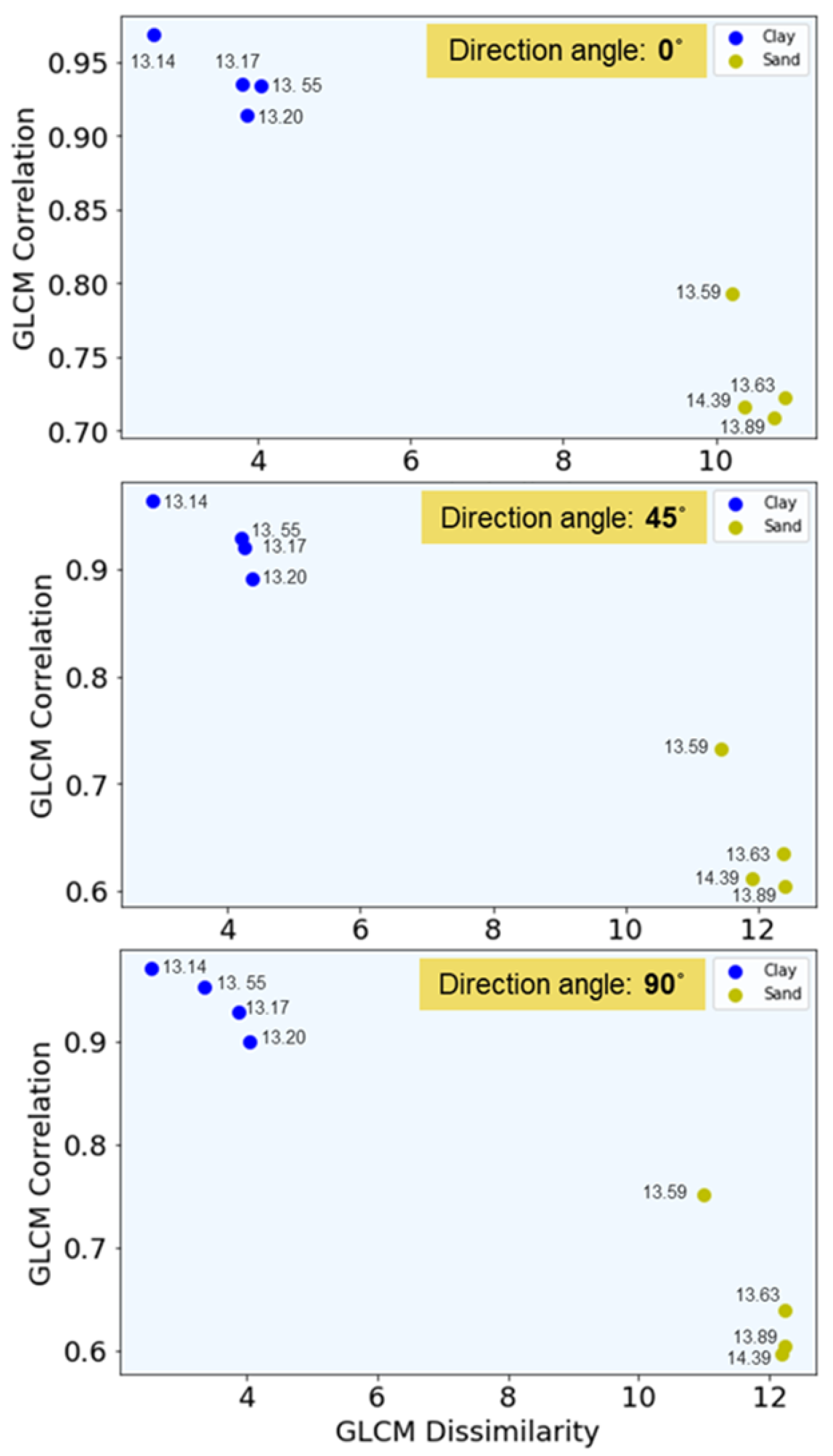
The two previously discussed features were extracted for each frame: GLCM correlation representing deformities in the image and GLCM dissimilarity representing its heterogeneity.

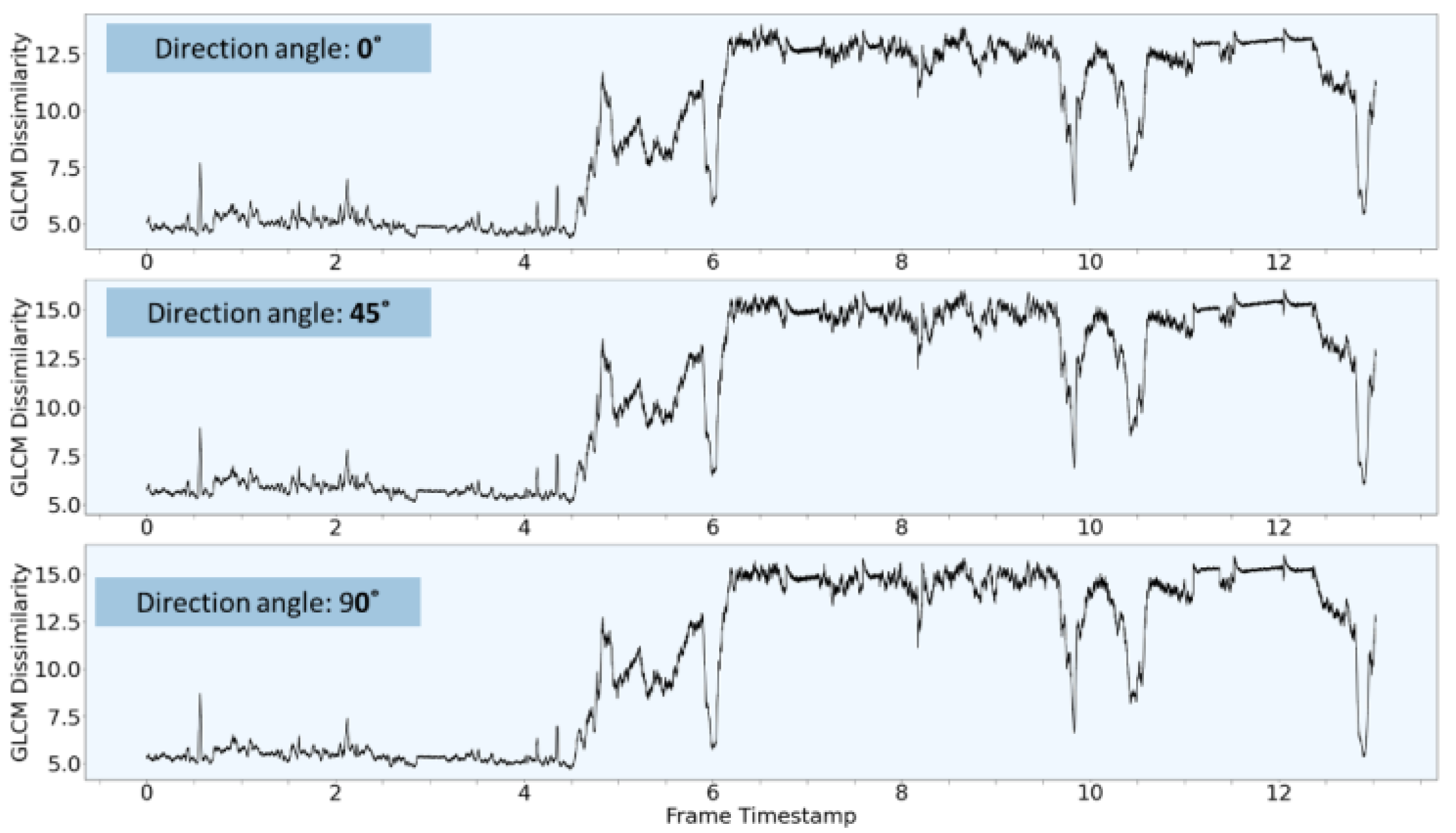
As seen in Figure 8, the difference between texture data is clearly visible. The frame denoting the camera depth of 13.14 m has the most regular texture among the clay frames, as does the frame at a depth of 13.59 m among the sand and clay frames. Clay images have small amounts of irregularity in texture, noted by high values of GLCM correlation, and different heterogeneity features noted by GLCM dissimilarity across all directions considered.

The result plots display minor differences in the values for three direction angles (Figure 8), while the frames representing both clay and sand are distinct with clear thresholds. This suggests that for the particular material recognition task in this particular case, specification of the direction value is irrelevant. However, this statement cannot be applied in all situations. For example, if the analysis aims to detect conveyor belt damage by analysing the surface of its ribbon, the GLCM direction choice is significant, as the area’s texture and deterioration will vary both across and along the ribbon.

Based on the conclusions from this first investigation based on a limited data set analysis, the entire video (i.e., all 19,540 frames) was processed. The results of this analysis are shown in Figure 9 and Figure 10. This chart not only demonstrates the insignificance of the GLCM direction choice for the current study aim but also illustrates noticeable thresholds indicating changes in soil types. For example, video sections corresponding to a low GLCM-Dissimilarity and a high GLCM-Correlation are likely to indicate soil with a very small grain size, such as clay. Contrary, video sections with high GLCM-Dissimilarity values and low GLCM-Correlation values correspond to more coarse grain sizes, such as what is typical for sand.

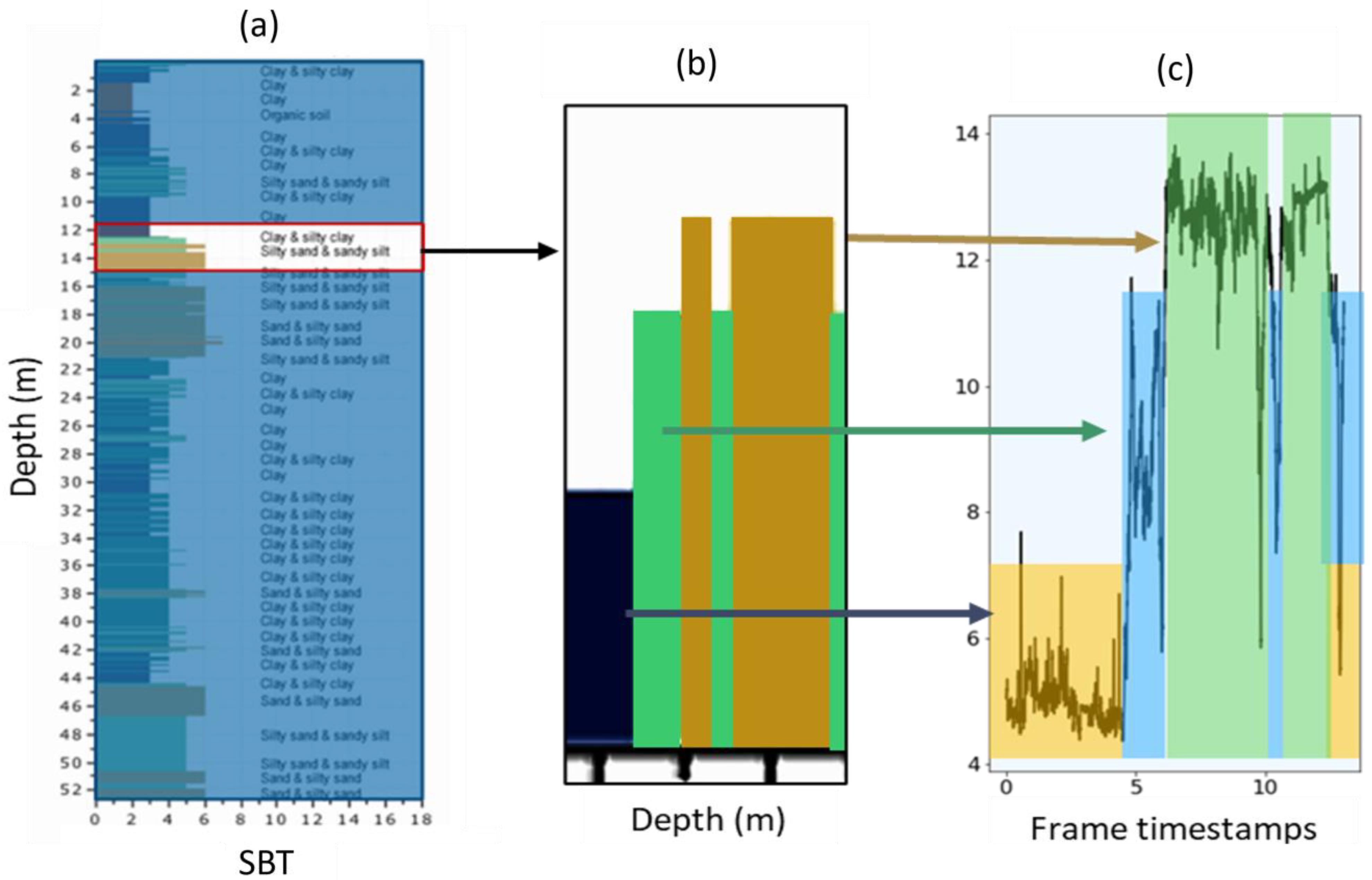
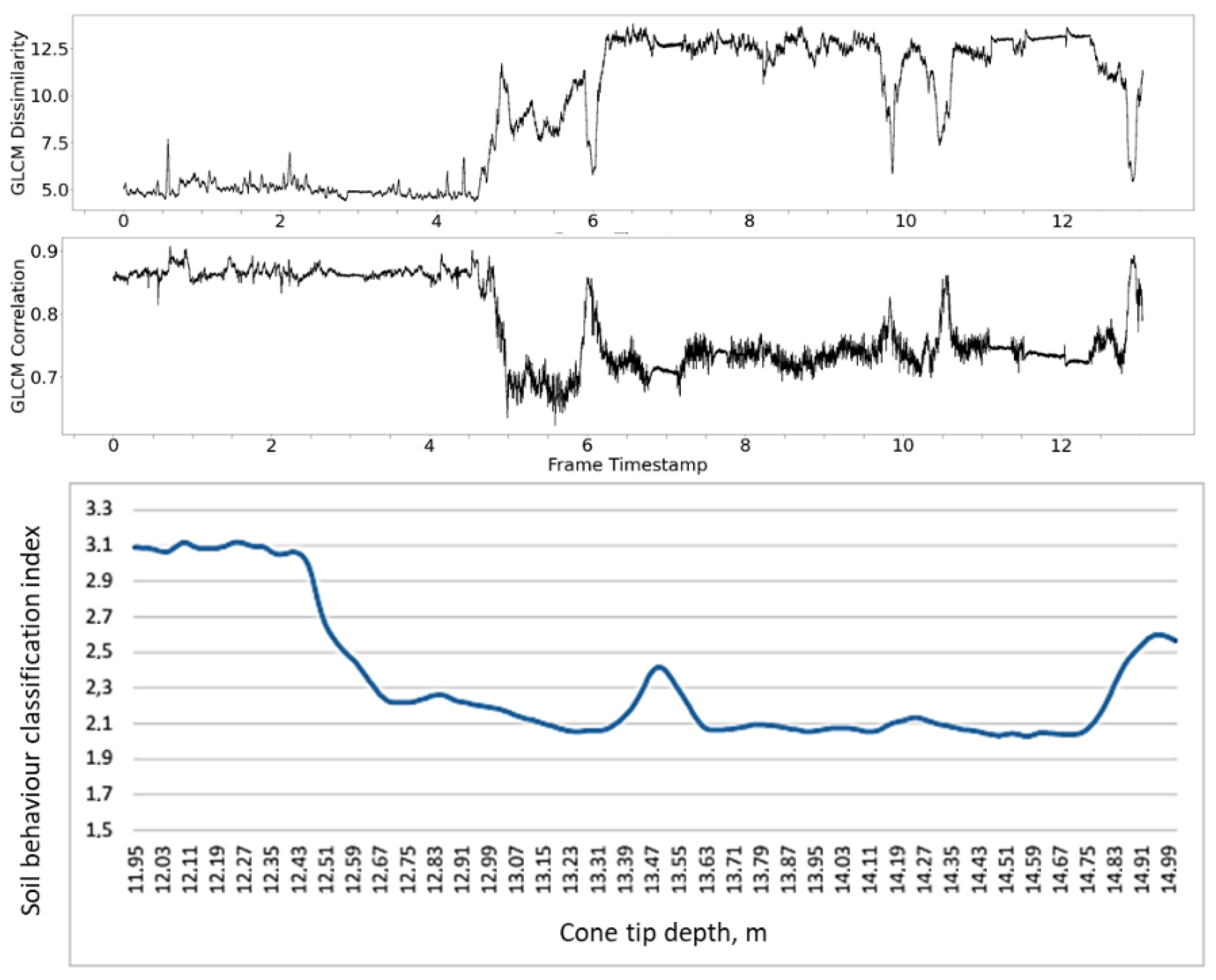
To validate the image analysis estimation, the created plots were compared to the soil behaviour type index derived from CPT data at the same location (Figure 11 and Figure 12). It is worth noting that the depth analysed in this research is only a part of the full CPT test, and this section was chosen given the noticeable change in the soil type predicted by the CPT data.

Image processing is obviously more sensitive to the texture or pattern type change than CPT results, as the images reflect the situation at a distinct depth, while the CPT data reflect a weighted average of the soil immediately ahead and behind the cone tip. But at the same time, the movement of the cone through soil may generate artificial structures and patterns that could appear in the video and could be misleading. The video quality and light conditions create additional noise, but this may be addressed by applying additional filters to the video.

Nevertheless, the two plots are visually similar and express similar thresholds that denote different soil types. Dissimilarity data contain less noise and more precise classification thresholds in comparison to the correlation image feature.

The Pearson correlation coefficient calculated for the CPT based Soil Behaviour Classification (SBC) and the GLCM correlation feature results in 0.62. This indicates moderate positive correlation between the two results.

The same coefficient between the SBC and the GLCM dissimilarity characteristic results in −0.6, which signifies a negative correlation, so that when one variable changes, the other variable changes in the opposite direction.

The correlation results are evident in Figure 12, where the grey level co-occurrence matrix correlation statistic closely aligns with cone penetration data in terms of peaks and drops. The dissimilarity statistic, on the other hand, offers greater precision and clarity in visualisation.

Note that this statistic was computed based on the 13 depth values datasets. The expansion and decoding of each depth value for both CPT and imaging data have great potential to generate a stronger correlation.

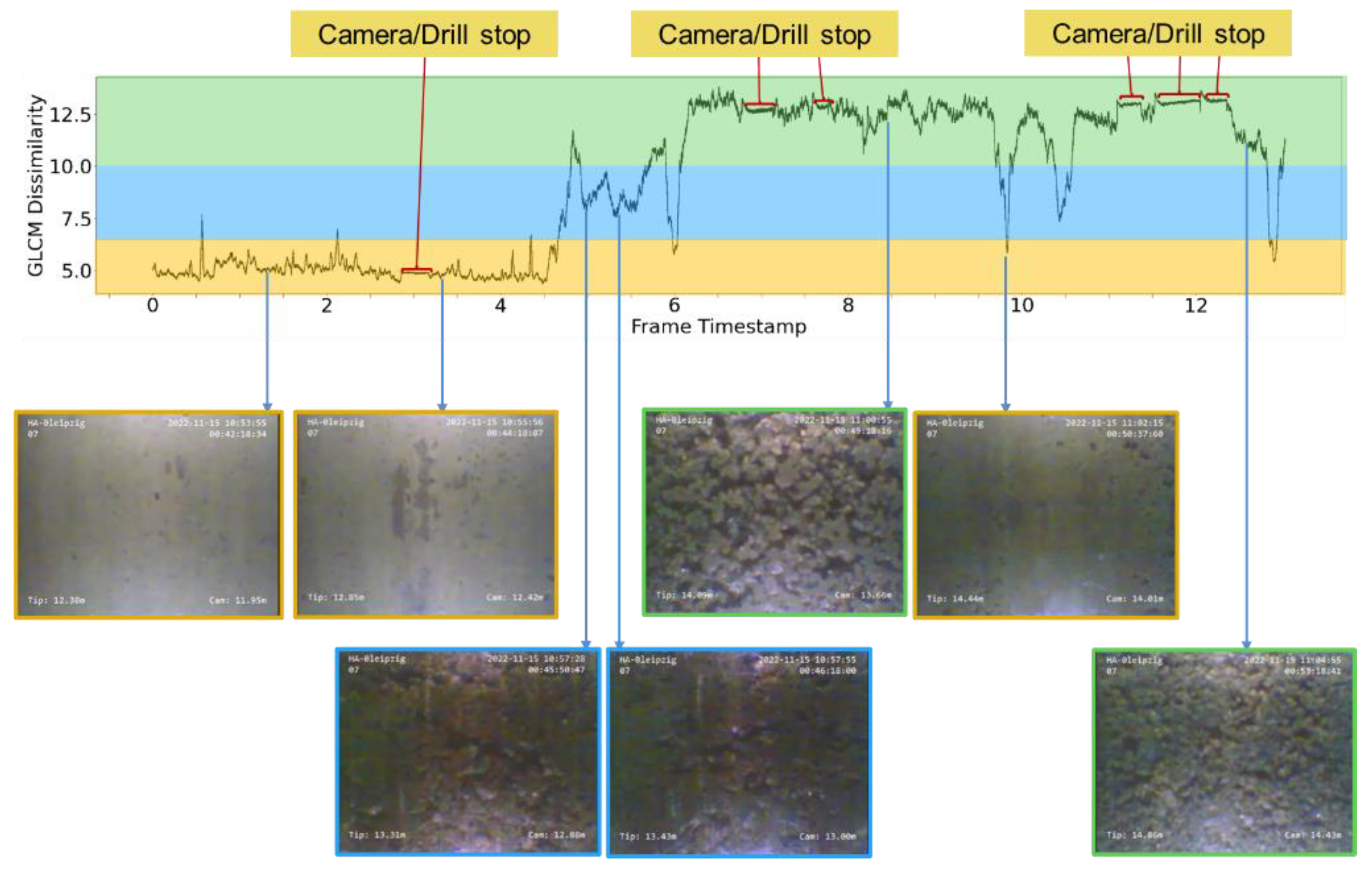
It should be noted that plots derived from image analysis results have zones with more or less static values. These zones are linked to pauses in the CPT cone penetration to add an additional tube at the surface to push the cone deeper into the soil (Figure 13).

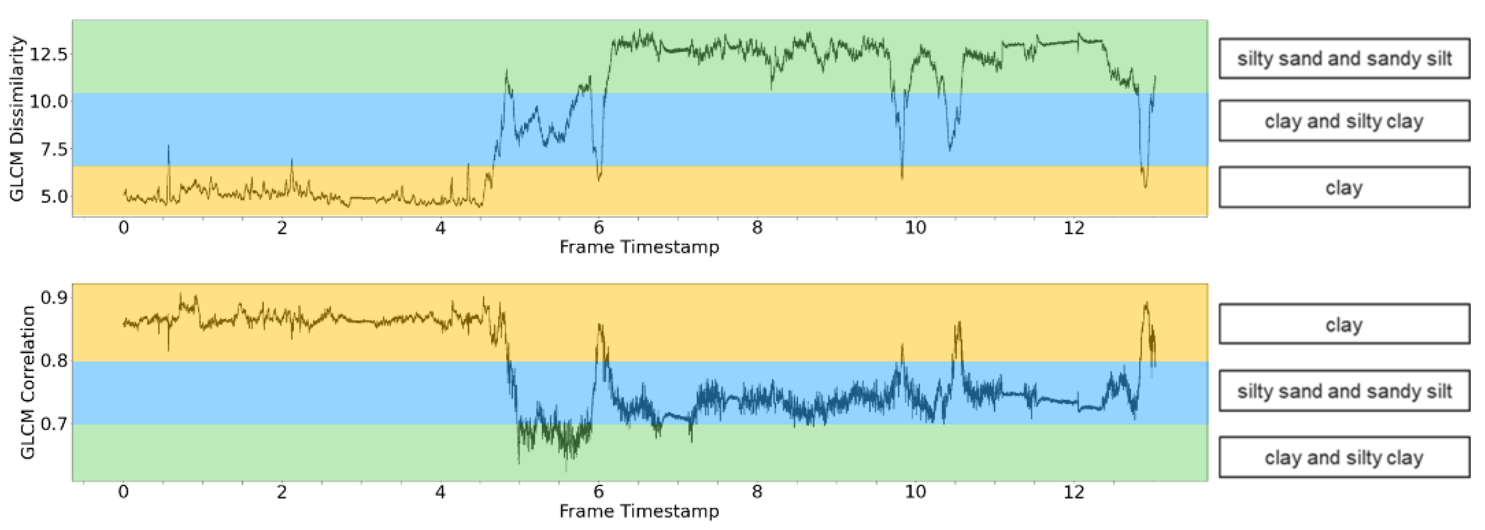
Both plots in Figure 14 show visible thresholds signifying textural image switching. As in the GLCM dissimilarity texture feature plot, three discrete texture zones are visible and are linked by timestamps in the video to three materials:

• [5–7]—clay (on the plots marked as yellow)
• [7–10.5]—clay and silty clay (on the plots marked as green)
• [10.5–14]—silty sand and sandy silt (on the plots marked as blue)

Within the GLCM correlation texture feature plot, two previously discrete texture zones, linked to silty clay and sand, are closer in values. Therefore three material texture zones have correlation values:

• [0.6–0.7]—clay and silty clay (on the plots marked as green)
• [0.7–0.8]—silty sand and sandy silt (on the plots marked as blue)
• [0.8–0.9]—clay (on the plots marked as yellow)

This study suggests significant potential to further develop applications of image analysis in various identification and characterisation tasks for soil material characteristics. With increasing camera resolution, it is expected to observe and detect not only the material surface, but also its details in the form of composition, inclusions, deformations and so on.

The analysis of a 13 min video using the Python programming language requires 25.8 s for processing each frame and a total of 29.9 s for overall processing, including library import, frame processing, visualization, and Excel conversion. This efficiency is demonstrated on a laptop equipped with an 11th Gen Intel Core i7 processor and 16 GB of installed random-access memory (RAM), affirming the time effectiveness of the method.

4. Conclusions

Image analysis can successfully recognize different soil types using its texture feature out of the recorded video file.

The use of the grey level co-occurrence matrix for material type identification reveals an efficient way to benefit from the soil investigation within minutes of the analysis; it provides a good proxy for the recognition of the material, estimation of its structure and distinct thresholds where the material type is changing. As such, the video recordings during a CPT investigation offer an independent source of information.

The accuracy of these results was confirmed through visual validation using video footage, as well through comparison with the Soil Behaviour Classification based on CPT data. The calculated correlation coefficient of texture features and SBC values show moderate correlation. Enhancing this validation process can be achieved by establishing a timestamp system during the soil investigation operation. This system will effectively link video timestamps with depth, CPT progress and SBC values, further improving the validation process.

Incorporating artificial intelligence such as Convolutional Neural Network models can boost the image recognition technique by providing expanded abilities, not only to recognize material change during video recordings of various operations, but also to provide advanced classification and characterisation of recorded material.

Considering the set up and data set studied in this research, the technique can be adapted to various mining environments. As the camera was installed on the video cone recording the CPT sounding process, the similar installation of a camera and the resulting video data can be used over a conveyor belt for material tracking or a dump model evaluation.