Design of Multi-Stage Solvent Extraction Process for Separation of Rare Earth Elements

Abstract

Flowsheet design and stage determination for the separation of rare earth elements (REEs) using solvent extraction (SX) is a challenging task because of the chemical similarity of the REEs. Low separation factors between the elements and complex equilibrium chemistry provide unique challenges to designing an efficient flowsheet for the separation of elements. The multi-stage nature of the SX process adds further complexity, making the assessment of products for a proposed design and stage combination difficult. Therefore, to develop a SX flowsheet, it is essential to quantify the performance for various design and separation conditions. This paper attempts to address the challenge by utilizing an equilibrium and process modeling approach. Results from a bench-scale study performed on a 10 g/L rare earth salt mixture were used in studying the extraction/stripping behavior and developing equilibrium models. DEHPA with TBP as a phase modifier was used as an extractant, while hydrochloric acid was utilized as a stripping agent. The results obtained were used in developing extraction/stripping models, which were integrated into a process framework of a SX train in a Matlab/Simulink environment. The models were programmed as a function block routine and used for developing a flowsheet, which was simulated for differing separation and design conditions. To identify optimum stage combinations, a particle swarm optimization (PSO) routine was developed and implemented for each SX train. Recovery and purity of elements of interest were used as objective function criteria. The stage combination leading to the minimization of the objective function was used to identify the optimum stage combination for a series of SX trains to attempt a balance of purity and recovery. The models and optimization method were implemented to separate a feed mixture containing REEs, which indicated that 99.52 and 85.41 percent purity is achievable for Yttrium and Lanthanum separation using 8-12-3 and 10-3-5 stage combination for loading, scrubbing, and striping. The model also indicated difficult separability between neodymium, praseodymium, and cerium.

1. Introduction

Rare earth elements (REEs) have become a vital component of our present economy, enabling modern technologies such as electric vehicles, batteries, renewable energy, etc. [1]. Growing applications in high-tech equipment are resulting in an increased demand for this group of elements [2]. However, the availability of mineable resources, difficult separability, and associated processing economics have raised concerns about the ability to meet the escalating demands [3]. Restricted market supply has further increased demand, thereby increasing the criticalities of these elements in modern society [4].

To mitigate the associated challenges and facilitate future supply, significant research and industrial efforts are being directed toward exploring alternative sources and economical extraction methods for these elements. However, the separation of REEs into individual high-purity products is difficult owing to their chemical similarities. Currently, solvent extraction (SX) is the preferred process used in commercial production of REEs [5,6]. The process utilizes the difference in extractant (lixiviant) affinity towards individual REEs and is influenced by factors like acidity, extractant concentration, metal concentration, etc., to achieve selective separations. Despite industry adoption, the process requires a significant number of stages due to small differences in separation factors between the REEs. This provides ample opportunity to optimize the design and performance of SX systems through modeling.

A typical design of SX processes for the separation of metals is performed by utilizing equilibrium information by developing extraction and distribution isotherms via experimental methods [7]. Extraction isotherms are used in identifying suitable pH, whereas utilizing distribution isotherms with an operating line (also known as the McCabe–Thiel method) is used as a graphical means for stage determination. This method is suitable for single-element systems where the co-extraction of undesired elements is negligible. However, multi-element co-extraction in REE systems presents a more complicated problem. The application of process modeling for REE process design does not appear extensively discussed in the open literature [5] and is corroborated by more recent works [8]. This paper attempts to bridge that gap by developing and integrating equilibrium models with process models for a complex REE system to aid in flowsheet design for REE separation. Subsequent sections further discuss the gaps within the equilibrium method, equilibrium models, and process modeling approach previously taken and how it attempts to fill the gaps.

1.1. Aqueous Organic Equilibrium

Extraction of REEs using SX is an equilibrium chemical reaction occurring across two different liquid phases, i.e., aqueous and organic. The reaction is reversible in nature, and the extent of the reaction is dependent upon the activities of species at equilibrium. For convenience, a trivalent form of the REE ion is depicted for loading into the organic phase with an acidic extractant as given by:

$${\mathrm{M}}^{3+}+\mathrm{n}{\mathrm{H}}_2{\mathrm{R}}_2\leftrightarrow \mathrm{M}{\mathrm{R}}_3(\mathrm{H}\mathrm{R}{)}_{2\mathrm{n}-3}+3{\mathrm{H}}^{+}$$

(1)

Equation (1) is a suitable approximation under trace concentrations. However, the REEs exist as different charged species in solution, which interact differently with polymeric forms of an extractant, resulting in multiple simultaneous reactions for each element and its species. For this reason, care must be taken when using the stoichiometry or chemical equilibrium reaction constant derived using the slope analysis method for flowsheet design, as they represent an ideal case. At high dissolved ion concentrations or when multiple ionic species exist in solution, as in the case of REEs, the fractional stoichiometric coefficients are observed [9,10], and the equilibrium reaction constant related to each ionic species should be considered. Additionally, equilibrium experiments (for distribution isotherms) are often conducted for single salt solutions, which fail to capture the effect of multiple-element interactions. In industry, more useful measures are defined in terms of the ratio of metal concentration between the aqueous and organic phases, referred to as distribution ratio (D_M), or percent metal extracted to the organic phase to originally contained in the aqueous phase, referred to as percent extraction (E_M) is used. The distribution ratio is mathematically expressed as:

$${\mathrm{D}}_{\mathrm{M}}=\frac{\left[\mathrm{M}{\mathrm{R}}_3\right(\mathrm{H}\mathrm{R}{)}_{2\mathrm{n}-3}{]}_{\mathrm{o}\mathrm{r}\mathrm{g}}}{[{\mathrm{M}}^{3+}{]}_{\mathrm{a}\mathrm{q}}}$$

(2)

with [ ] denoting concentrations of the respective species [11]. The distribution ratio may be viewed as a suitable simplification of the aggregated effects of multiple ionic states due to the non-ideal behavior of an element found in the system. Whereas percent extraction is expressed as:

$${\mathrm{E}}_{\mathrm{M}}=\frac{\left(\frac{{\mathrm{V}}_{\mathrm{o}}}{{\mathrm{V}}_{\mathrm{a}\mathrm{q}}}\right)\times {\mathrm{D}}_{\mathrm{M}}}{\left(\frac{{\mathrm{V}}_{\mathrm{o}}}{{\mathrm{V}}_{\mathrm{a}\mathrm{q}}}\right)\times \left({\mathrm{D}}_{\mathrm{M}}+1\right)}$$

(3)

where V_o and V_aq are volumes of organic and aqueous phases (or flowrate in case of continuous process), and D_M is the distribution ratio [7]. From Equation (3), it is notable that the percent extraction of a metal is dependent on phase and distribution ratios. This expression is useful to determine the influence of both the pH and phase ratio on the extraction of multiple REEs.

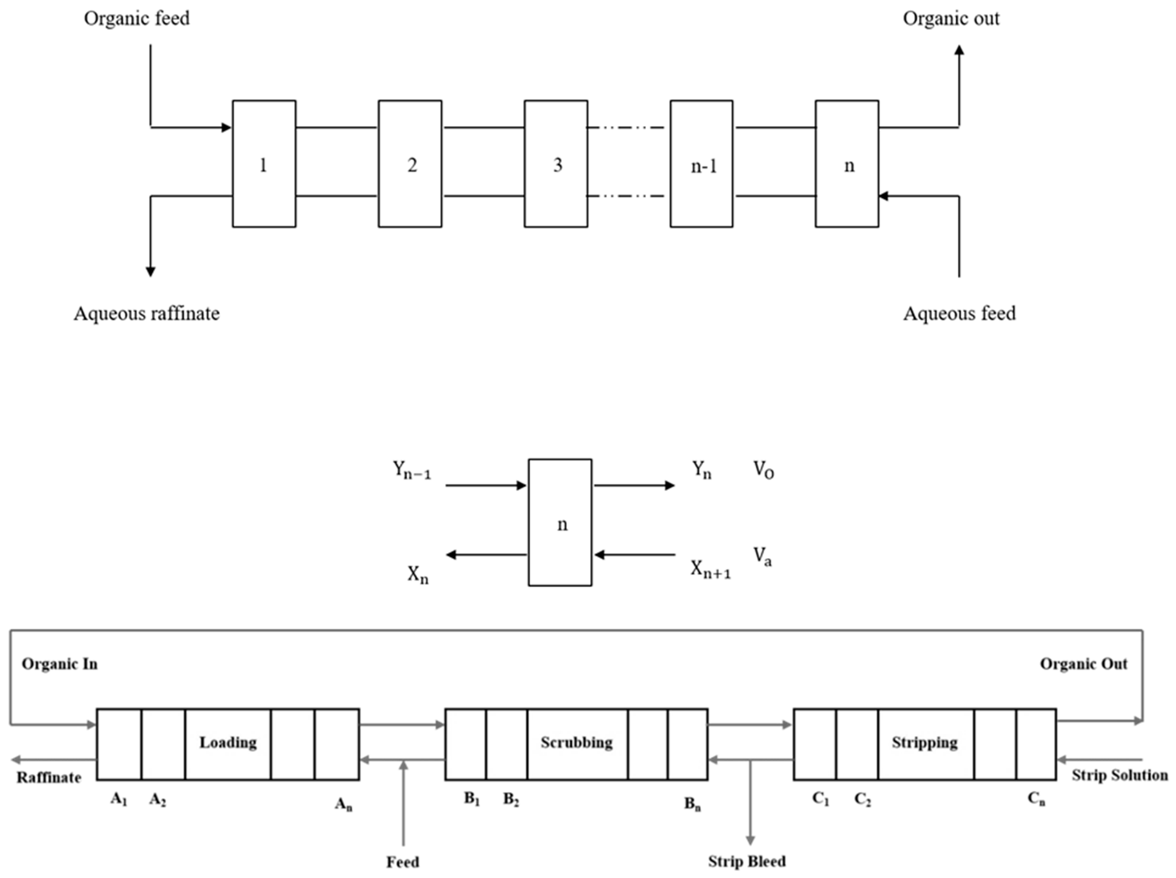
1.2. Counter-Flow SX Configuration and Design

While several circuit configurations are possible with SX, the counter current SX setup is widely used in metal separation due to high efficiency from multiple contacts between organic and aqueous phases (Figure 1). A typical counter current SX circuit would contain a combination of stages for loading, scrubbing, and stripping the metal from the feed solution. The three processes interact as the aqueous and organic solution flow in opposite directions, leading to selective extraction and stripping based on process conditions.

Design procedures relating to the SX process can be traced back to multi-stage chemical process design, such as distillation and vaporization columns. Typically, the development of the process models for counter-current SX configurations considers mass balance across a single stage of an “n” stage SX process, as shown in Figure 1. The mass balance for a metal is expressed using concentration and flow variables, shown in Equation (4), where Y and X followed by a subscript represent the concentration in the organic and aqueous phase, the subscript indicates the stage number, and V_o and V_a represent volumetric flowrate of organic and aqueous phases [5,12].

$${\mathrm{Y}}_{\mathrm{n}}{\mathrm{V}}_{\mathrm{O}}+{\mathrm{X}}_{\mathrm{n}}{\mathrm{V}}_{\mathrm{A}}={\mathrm{Y}}_{\mathrm{n}-1}{\mathrm{V}}_{\mathrm{O}}+{\mathrm{X}}_{\mathrm{n}+1}{\mathrm{V}}_{\mathrm{A}}$$

(4)

Two methods have been primarily used to solve the above equation for SX mass transfer: graphical and algebraic. The first method, known as McCabe–Thiele (MT), is a well-established graphical approach and is generally practiced by developing extraction and distribution isotherms and is particularly suited to single-element extractions. Multiple elements increase the number of assumptions required to construct the operating line, leading to ambiguity in the solution. The second method is an algebraic method and uses distribution coefficients derived experimentally or theoretically to solve for the concentration of metal in streams leaving the system. This method was originally developed by Kremser and is known as the Kremser equation [13,14]. In the Kremser method, the solution to Equation (4) is approached using a simplifying assumption of zero metal concentration of metal in organic feed entering stage 1 of the SX train (Y₀ = 0, Figure 1 when n = 1). This simplification results in the following equation form for stage 1 with one less unknown:

$${\mathrm{X}}_2={\mathrm{X}}_1+\left(\frac{{\mathrm{V}}_{\mathrm{O}}}{{\mathrm{V}}_{\mathrm{a}}}\right)\times {\mathrm{Y}}_1$$

(5)

The transfer or extraction of metal in the stage is then expressed by a constant distribution coefficient, as shown in Equation (6), which, upon substitution to Equation (5), results in Equation (7).

$$\mathrm{D}=\frac{\mathrm{Concentration}\mathrm{of}\mathrm{metal}\mathrm{in}\mathrm{organic}\mathrm{outlet}}{\mathrm{Concentration}\mathrm{of}\mathrm{metal}\mathrm{in}\mathrm{aqueous}\mathrm{outlet}}=\frac{{\mathrm{Y}}_{\mathrm{n}}}{{\mathrm{X}}_{\mathrm{n}}}$$

(6)

$${\mathrm{X}}_2={\mathrm{X}}_1\times (1+\frac{{\mathrm{V}}_{\mathrm{O}}}{{\mathrm{V}}_{\mathrm{a}}}\mathrm{D})$$

(7)

The lumped parameter (V_O/V_a)$\mathrm{D}$ is often referred to as an extraction factor (E) for simplicity, indicating the ratio of the mass flow rate of metal in the outlet to the inlet stream. However, it should not be confused with the percent extraction described in Equation (3), which is relative to feed. The process, when extended to n stages, leads to the following form [12]:

$${\mathrm{X}}_{\mathrm{n}+1}={\mathrm{X}}_1(1+\mathrm{E}+{\mathrm{E}}^2+\cdots {\mathrm{E}}^{\mathrm{n}})$$

(8)

$${\mathrm{X}}_{\mathrm{n}+1}={\mathrm{X}}_1\times \left(\frac{{\mathrm{E}}^{\mathrm{n}+1}-1}{\mathrm{E}-1}\right)$$

(9)

The Kremser method solves Equation (8) via a geometric sequence sum approach where the ratio between two consecutive terms is a constant, ‘E’. This equation can be solved for any number of stages (n) provided the feed and raffinate composition are known. The Kremser method is useful in designing a simple process involving single ionic states as it utilizes the distribution coefficient of elements and assumes a constant extraction factor across stages. The assumption of a constant distribution coefficient across multiple stages and zero concentration (fully stripped) returning organic phase entering stage 1 is not typical of SX trains involving loading, scrubbing, and stripping processes.

1.3. Application of SX Modeling in Design

As noted, the extraction of REEs is not trivial, and simplistic methods do not lend themselves to accurate predictions. Various methods of modeling SX equilibrium have been proposed which includes thermodynamic approaches, regression methods, neural networks, etc. [13,14,15]. The models are simple in terms of usability and mostly predict the elemental distributions; however, the independent variables used in developing these models are not consistent. For example, Thakur [13] used empirical models of an exponential form to predict distribution ratios as a function of the initial acid and metal concentrations. In contrast, Giles et al. [15] used an artificial neural network with the crystal radius of the lanthanide elements to generalize the separation behavior of rare earth SX processes. Early work by Sharp and Smutz [16] utilized separation factors for single stages and then proposed a methodology for application to multiple stages utilizing equilibrium and the operating line to alternatively determine concentrations in the various streams. It is noted that in certain circumstances, what appear to be numerical instabilities occurred. However, in the presented work, the comparison to experimental data showed good agreement. Sebenik with Sharp and Smutz [17] extend their work to a 5 REE system utilizing the same methodology, showing the convergence of the iterative loop utilizing equilibrium and operating lines. Later work includes Voit [18], which used the Kremser method to determine the concentration of various streams in the circuit. The model required input parameters such as feed composition, separation factors, number of stages, and reflux ratios. Reddy et al. [19] utilized a similar approach to Kremser with separation factors, feed composition, and equilibrium data to simulate different stages and phase flow rates. The limitation of these approaches is the analysis of a single SX train and those inherent to the Kremser method. Further, these do not account for the extraction change due to phase ratio change. Another simulation method developed by Wenli et al. [20] was based on a coupled analytical method (EDXRF) with flowsheet modeling. The model requires such variables as feed composition, extractant, separation factors, separation indexes required, and number of stages. From the reported work, it appears that this work would be specifically utilized for monitoring rather than for flowsheet design. For comparison, examples from cobalt/nickel systems developed by Cytec, such as Minchem for SX flowsheet simulation and process improvement, are also considered, as reported by Bourget et al. and Soderstrom et al. [21,22]. The work involved simulating a flowsheet for a range of operating parameters and stage combinations for optimizing the pH profile and maximizing cobalt recovery. In Bourget’s work, a type of pre-generated equilibrium data is used, but the exact nature of the multi-stage model is not given. Similarly, Evans et al. [23] reported the use of the Aspen Custom Modeler for cobalt/nickel separation. The work utilizes an equilibrium constant within the framework of the Aspen process modeling software to optimize the cobalt extraction and minimize magnesium and nickel co-extraction. As mentioned before, the estimation of the equilibrium constant is based on experiments conducted on a low salt solution, which may not accurately represent high concentration conditions. Returning to REEs, further validation shows what appears to be a collaboration with Cytec. Lyon et al. [24], in comparing reagent performance for group separation of REEs, used modeling based on separation factors. The software used equilibrium curves but was limited to single trains and did not consider phase ratios and variable stage combinations. A more recent development by Turgeon et al. [8] in REE separation utilized both estimated equilibrium constants and an algebraic set of equations to solve the equilibrium conditions. This model, however, does not address optimization. For convenience,

Table 1. Programs developed for process modeling of SX.

Metal	Year	Method	Tool	Name
REEs	1965	Separation Factor	Stage-wise iterative calculation	[16]
REEs	1966	Separation Factor	Stage-wise iterative calculation	[17]
Nd	1989	Kremser	Solution of Kremser Method	[19]
REEs	1992	Kremser	Solution of Kremser Method	[20]
REEs	2000	Online Analytical Measurement	ESRECE simulation system	[21]
Cobalt/Nickel/Copper	2010	Equilibrium Type	by Cytec (no name)	[22]
Cobalt/Nickel	2011	Equilibrium Type	MINCHEM (Cytec)	[23]
Cobalt	2014	Equilibrium Type	Aspen custom modeler	[24]
REEs	2023	Equilibrium Constants	Algebraic Mass Balance	[8]

lists and summarizes select examples of previously developed tools and equilibrium methods used in SX process modeling.

From the preceding discussion, it is evident that modeling a REE system is challenging because of multiple similar extracting elements. In most of the recent works, a combination of equilibrium modeling used in conjunction with multi-stage concentration determination is utilized. Save for Turgeon et al. [8], none have attempted more than a single SX train, and none of these works have attempted an optimized solution. It is clear that a more consistent approach to independent variable selection based on fundamentals applied across SX trains would be beneficial. Further, very few of the discussed equilibrium models have been utilized as SX design tools.

1.4. Gaps and Approach

As previously discussed, it is clear that the design of a SX process to effectively separate REEs is a complex multivariate problem, as summarized in Figure 2. To provide the practitioner a means for configuration and stage determination of a multi-stage SX flowsheet for the separation of REEs into individual high-purity products, a novel simulation method integrating equilibrium information and process modeling is proposed. The method utilizes Matlab’s Simulink, which is modular and can be used for the flowsheet design of many SX configurations. An optimization algorithm based on particle swarm methodologies is proposed to determine the number of stages for user-defined optimization criteria based on recovery, purity, or both. The method proposed is as follows:

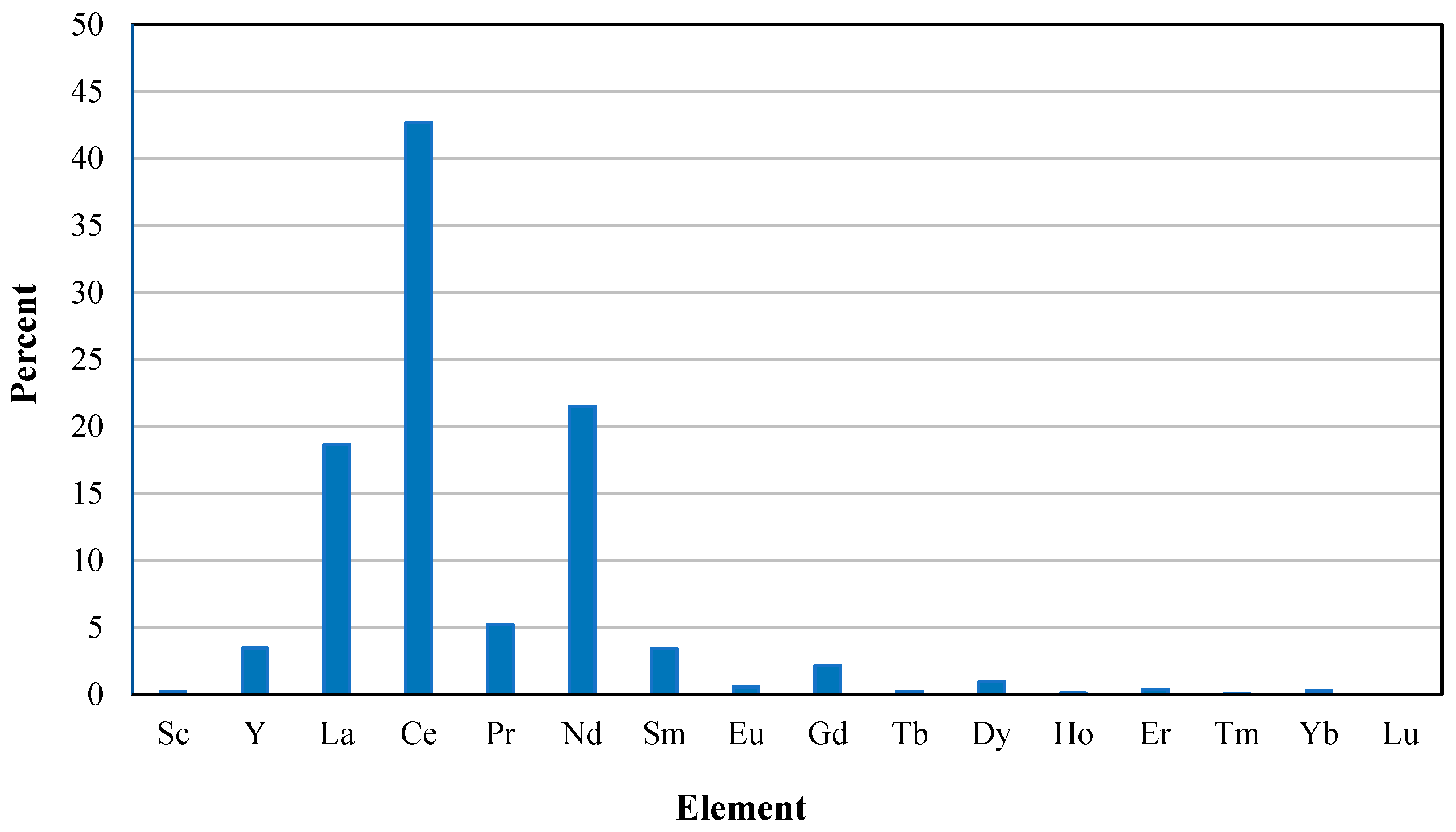
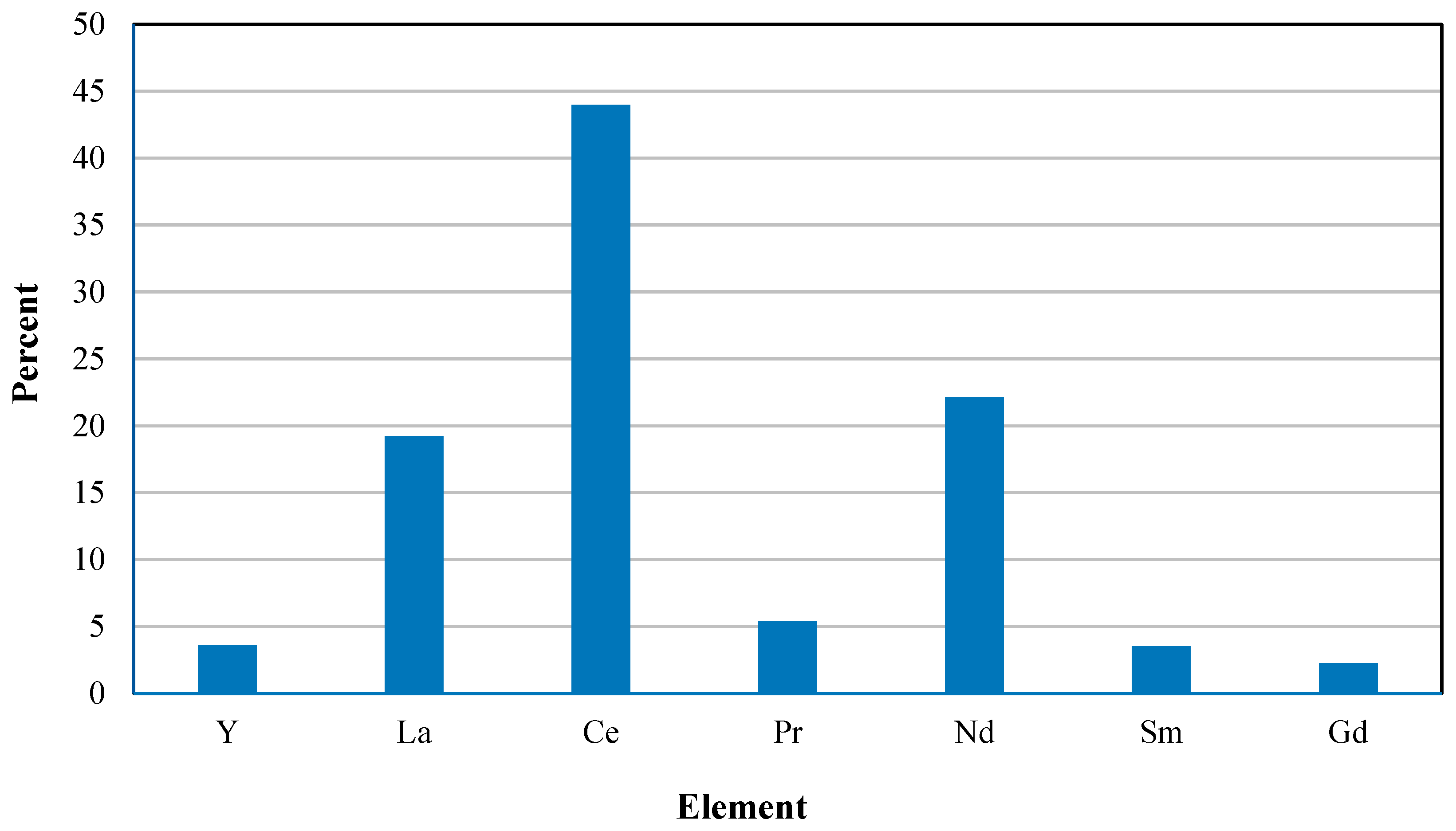
• Identify the initial SX feed characteristics considered for design (REE concentration in this case);
• Determine the ideal pH to achieve separation using bench-scale equilibrium experiments;
• Perform a circuit layout composed of specific SX “trains” defined as loading, scrubbing, and stripping;
• Determine the ideal phase ratio for improved separation, thereby holding the phase flow parameters constant, using bench-scale equilibrium experiments as the basis for developing equilibrium regression models for these variables;
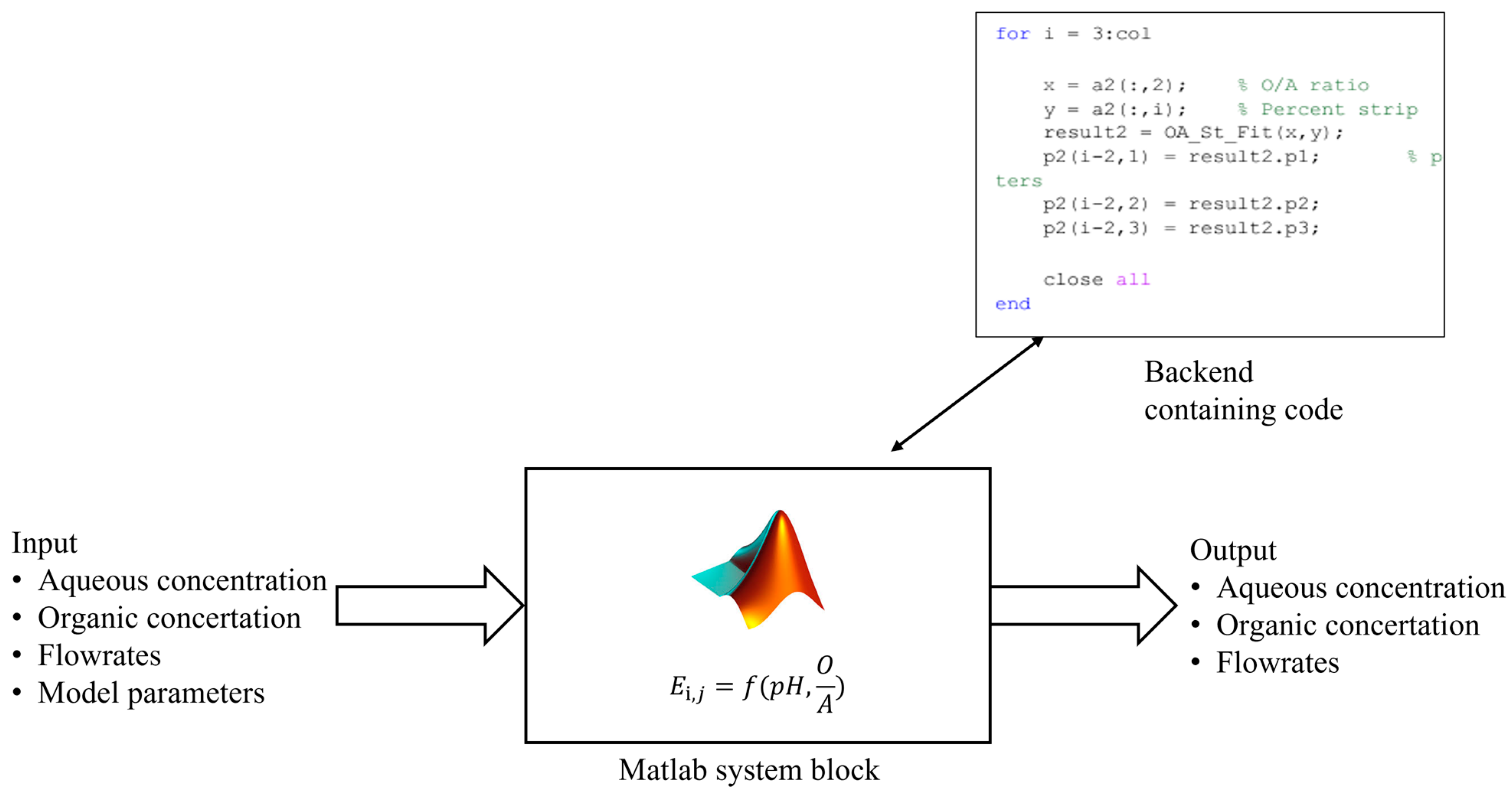
• Develop stagewise arithmetic determination of an equilibrium utilizing MATLAB Simulink as blocks corresponding to discrete functions such as loading, scrubbing, and stripping;
• Perform by training a particle swarm optimization method to design and simulate a flowsheet and determine the number of stages needed for separation on the basis of recovery and/or purity.

The specific reasoning for the approach will be given as part of the model description. The accomplishment of these objectives is described in this paper in four parts. The first involves the development of the theoretical framework of the model and lays the foundation for the needed inputs (corresponding to the theoretical aspects of items 5 and 6 above). The second covers the selected SX inputs, develops the purpose of the modeling exercise, and discusses the pH selection (items 1–3 above). The third develops the phase ratio and extraction equilibrium methods needed for the model (corresponding to item 4). This includes the methods and materials covering the experimental aspects of this work to generate the data to model. Lastly, the optimization objectives and specific approach are discussed in part four, entailing the specific development of a REE roughing circuit (items 5 and 6). As this study is intended to be a discussion on SX design and optimization, the results will be illustrative of the utilization and initial concept design of a REE roughing circuit with the performance objective of maximizing recovery and purity simultaneously.

2. Materials and Methods

2.1. Part 1: Development of Modeling Theory and Methods

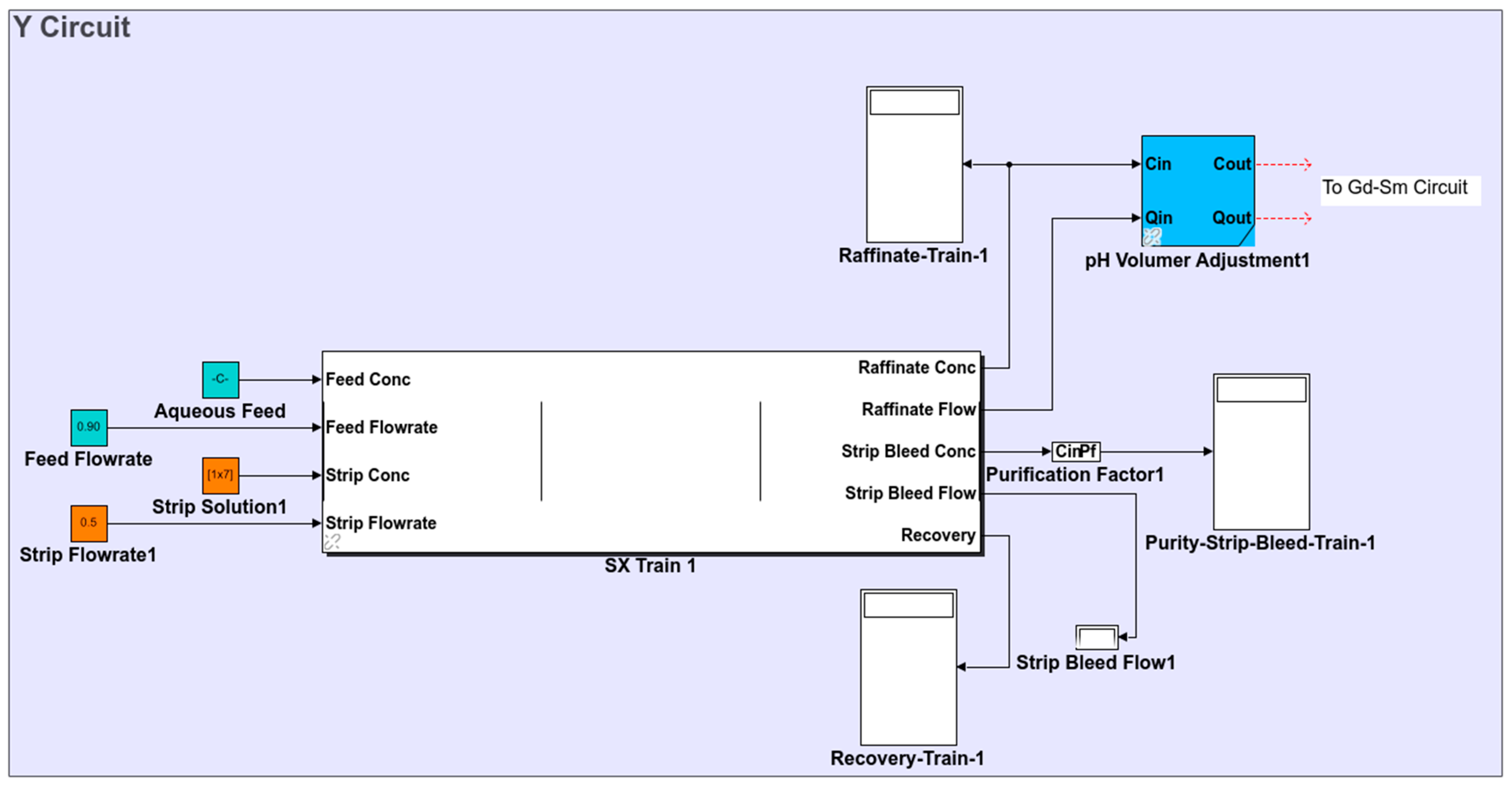
2.1.1. Circuit Definition

A SX “train” is defined for convenience as a series of SX stages comprising loading, scrubbing, and stripping, as shown in Figure 1, which utilizes a reflux from the stripping stage. This was selected as reflux minimizes dilution of aqueous feed compared to a barren scrub solution, thus increasing the effectiveness of separation [5].

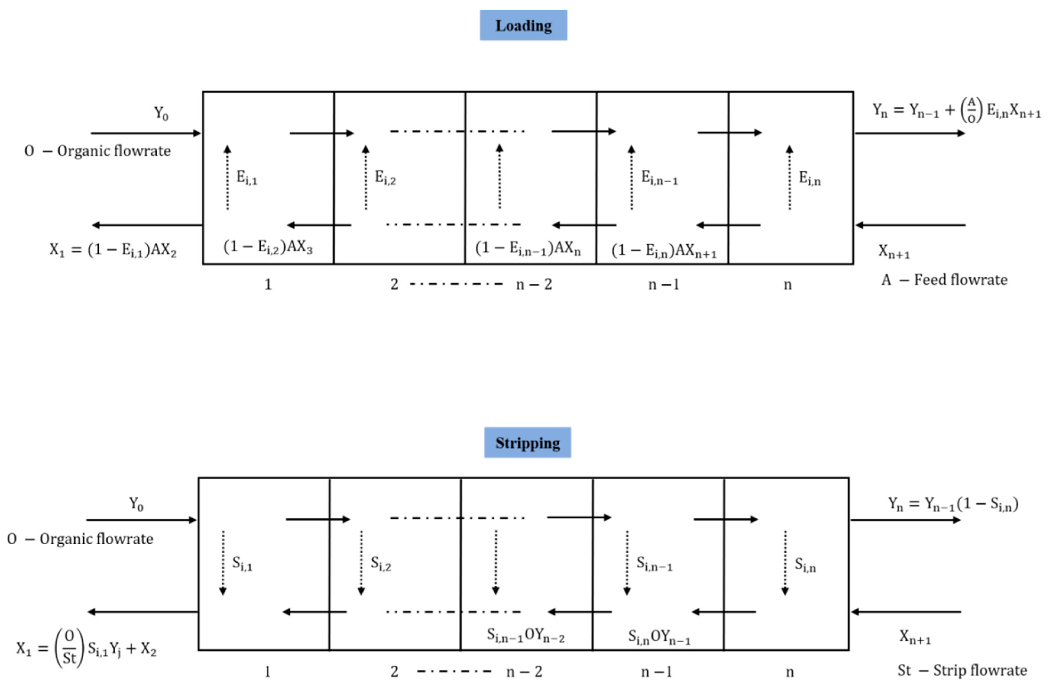
2.1.2. Algebraic Mass-Transfer Definition

To predict stagewise mass transfer of the elements in a SX train for a given separation condition, process models were developed via first-principle mass balance. The mass balance equations for a single stage were developed by rearranging Equation (4), as shown in Figure 3. The phase ratio models defined in Part 3 are utilized to solve for the metal transfer for an individual stage for pH and phase ratio conditions existing in the stage. This method was extended to multiple stages, wherein the stagewise solution from one stage served as the input feed concentration condition to the next Figure 4. The nomenclature for symbols used follows the same convention as described previously. For scrubbing, the method developed for stripping was followed.

A general form of the equation to obtain the raffinate and loaded organic concentrations used in a loading process using the method shown in Figure 4 is given by:

$${\mathrm{X}}_1={\mathrm{X}}_{\mathrm{n}+1}\left(1-{\mathrm{E}}_{\mathrm{i},1}\right)\left(1-{\mathrm{E}}_{\mathrm{i},2}\right)\dots (1-{\mathrm{E}}_{\mathrm{i},\mathrm{n}})$$

(10)

$${\mathrm{Y}}_{\mathrm{n}}=\left(\frac{\mathrm{A}}{\mathrm{O}}\right){\mathrm{X}}_{\mathrm{n}+1}\left[{\mathrm{E}}_{\mathrm{i},\mathrm{n}}+\right.{\mathrm{E}}_{\mathrm{i},\mathrm{n}-1}\left(1-{\mathrm{E}}_{\mathrm{i},\mathrm{n}}\right)+{\mathrm{E}}_{\mathrm{i},\mathrm{n}-2}\left(1-{\mathrm{E}}_{\mathrm{i},\mathrm{n}}\right)\left(1-{\mathrm{E}}_{\mathrm{i},\mathrm{n}-1}\right)\dots \dots ]+{\mathrm{Y}}_0$$

(11)

The above equation is an integrated form of all loading stages but was solved stagewise using the Simulink function block, where the output of one stage served as an input to the other. The E_i,n for each stage was predicted from a regression model fitted to experimental data discussed later utilizing pH and input flow conditions information of that stage. As organic is in recirculation, the Simulink utilizes an algebraic loop solver based on the trust region and line search method.

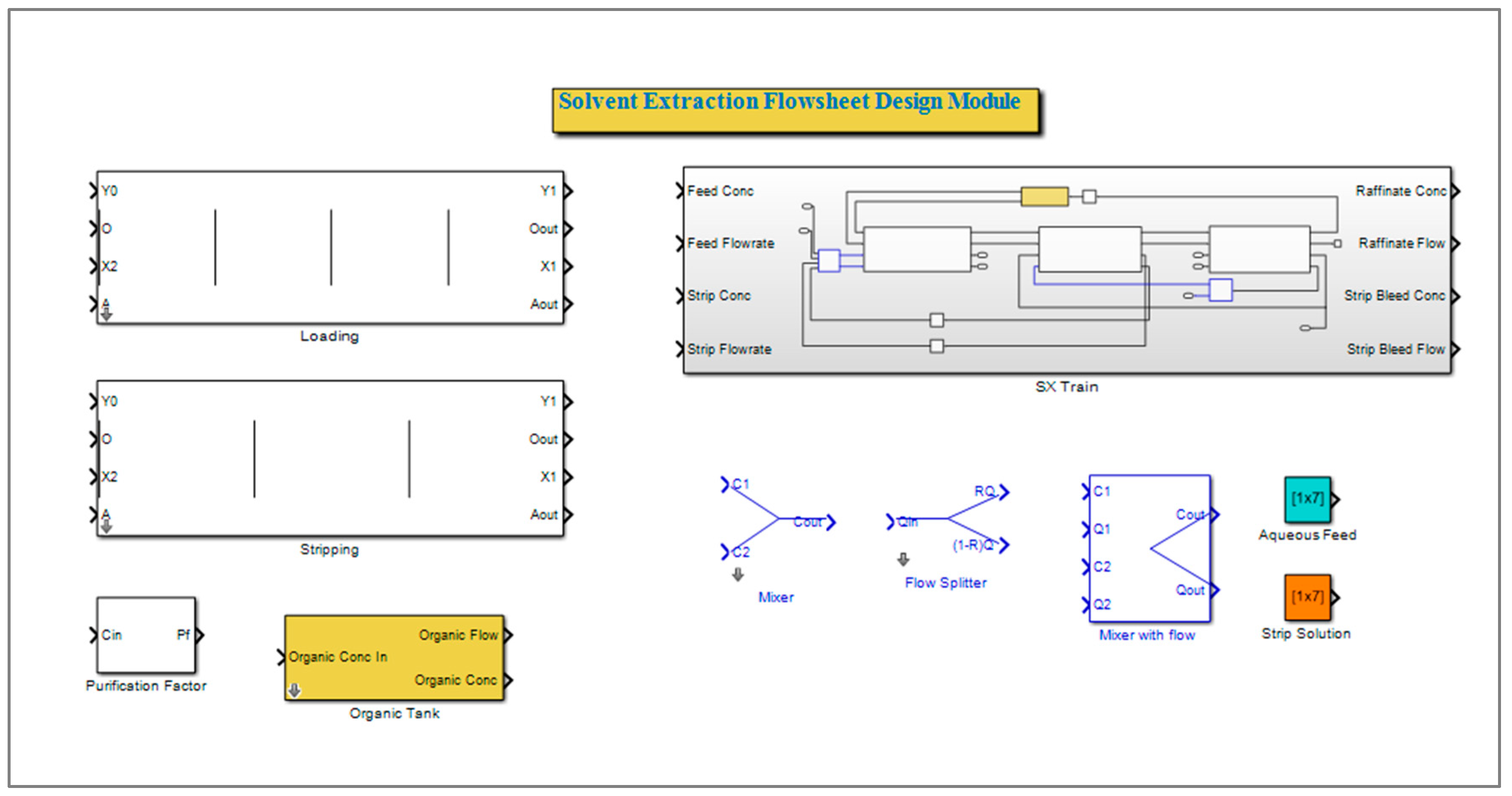
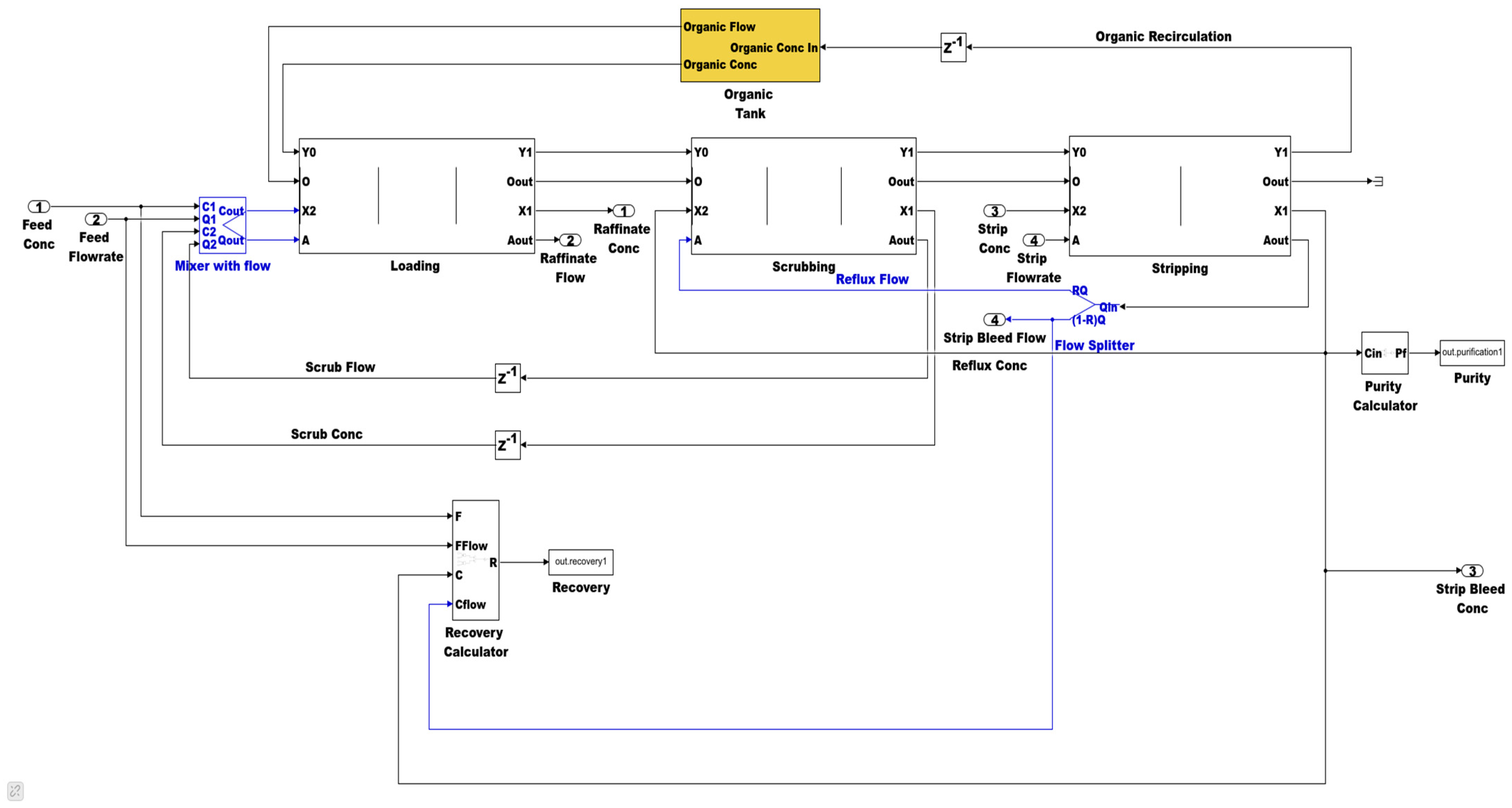
2.1.3. Simulink Library Development

To implement the process model and facilitate the flowsheet design process, the models were programmed in Simulink, and a model library was developed. Simulink is an application of Matlab widely used for modeling, designing, and simulating steady-state and dynamic processes. It has found wide application in numerous industries, such as mechanical and chemical, due to its ability to model systems as graphical function blocks [25]. A function block is essentially a computer program describing a process, and it contains input–output ports to pass inputs and receive processed outputs. Simulink allows features of connecting multiple independent function blocks through signal lines to transfer input–output between other function blocks. The block nature of modeling and the ability to interconnect multiple blocks allow for the easy integration of the two different processes. Figure 5 shows the working of a typical Simulink block, wherein the input information to the block is passed through connected signal lines or provided externally through code.

For SX flowsheet design involving multiple interacting processes such as loading, scrubbing, stripping, etc., the graphical nature of Simulink is of immense value. SX processes represented as graphical blocks can be easily configured to design and simulate SX flowsheets. Signal lines containing aqueous/organic concentrations and flow rate information can be used to transfer input–output information between connected blocks. In addition, the Simulink subsystem feature, which is a nested block function, allows for the reduction of multiple stages and processes to a single block, which improves flowsheet design efficiency. For the SX flowsheet design, a library containing graphical block models of different processes, i.e., loading, scrubbing, stripping, mixers, flow splitter, and pH regulator, was developed, as shown in Figure 6. The block contained code for each process developed using a combination of Matlab script and Simulink function s-functions and can be found in a previously published work [26]. The blocks were arranged to form a SX train block, which could be utilized multiple times by updating the separation conditions, thereby reducing the complexity in flowsheet design. Figure 7 shows an example of a SX train subsystem consisting of all function blocks interconnected to develop a SX train. The purity and recovery block models were also developed to evaluate the performance of the output stream and were evaluated using the following expressions:

$${\mathrm{P}}_{\mathrm{i}}=\frac{[\mathrm{M}{]}_{\mathrm{i},\mathrm{stream}}}{{\sum }_{\mathrm{i}=1}^{\mathrm{n}}[\mathrm{M}{]}_{\mathrm{i},\mathrm{stream}}}\times 100{\mathrm{R}}_{\mathrm{i}}=\frac{[\mathrm{M}{]}_{\mathrm{i},\mathrm{stream}}\times {\mathrm{f}}_{\mathrm{s}\mathrm{t}\mathrm{r}\mathrm{e}\mathrm{a}\mathrm{m}}.100}{[\mathrm{M}{]}_{\mathrm{i},\mathrm{f}\mathrm{e}\mathrm{e}\mathrm{d}}\times {\mathrm{f}}_{\mathrm{f}\mathrm{e}\mathrm{e}\mathrm{d}}}$$

(12)

where P_i and R_i represent the purification factor and percentage recovery of metal i, M_i the concentration of metal of interest i in the given stream, f_stream the flowrate of the subscripted stream, and n the number of metal species present in the stream.

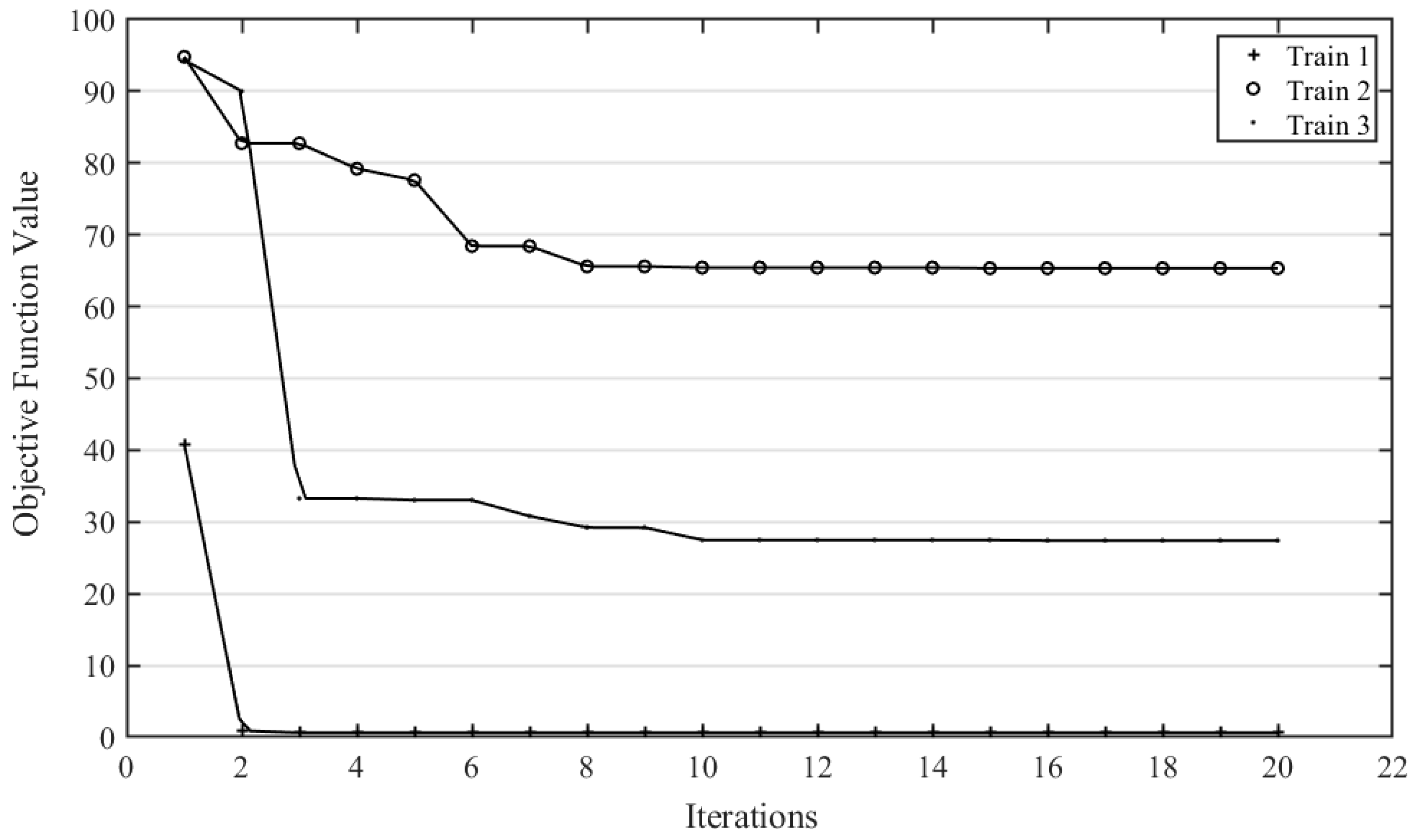
2.1.4. Particle Swarm Optimization Algorithm

Using the Simulink model library, the proposed conceptual flowsheet was designed in Matlab Simulink. Figure 8 shows an example SX train for Yttrium separation from feed mixture. The reason for this separation configuration will be given later and in greater detail. The flowsheet could be simulated for numerous stage configurations and operating conditions to explore the effects on separation and recovery. However useful, managing the output of such simulations can be difficult because of the large number of variables and complexity of the process. For this reason, optimization methods are applied in this work, which selects the ideal outcomes based on defined criteria using an objective function. For many REE separation flowsheets, the design goal is to identify the number of stages and requisite SX trains required to achieve the desired purity. Therefore, the optimization method can be applied to maximize the purity of a desired element in the output stream. Further compounding the design difficulty is that high purity often occurs at the expense of recovery. In this work, recovery, purity, or a combination are considered at different points of the flowsheet to assist in design. For this work, a particle swarm optimization (PSO) method was selected because of the discrete nature of the input variables, the non-linear nature of the process, and as a means to understand local versus global minima or maxima.

PSO is a heuristic optimization method used for mixed-integer, non-linear problems, and it is based on the social model of the flocking of birds or the schooling of fish [27]. The method uses a selected number of particles (birds, for example, in the social model) determined at the start of the optimization. The particles are characterized by position and velocity in multi-dimensional space dimensionality determined by a number of unknown variables for optimization. Every particle in the swarm searches for the optimum value in the multi-dimensional search space, with an optimum value representing the best value of the objective function attained by the particle. The particle identifies the position (p_best,i) associated with the respective optimum of the objective function (f_pbest,i) location. The particles then congregate, and the objective function value among the particles is compared, and the best objective function value (f_gbest) and associated position (p_gbest) achieved by the swarm are recorded. The process is repeated iteratively by updating the velocity and position of particles until the global optimum value has been reached. The velocity and position, initially chosen at random within provided boundary conditions, are updated by the following [27,28]:

$${{\mathrm{V}}_{\mathrm{i}}^{\mathrm{t}+1}=\mathrm{w}{\mathrm{V}}_{\mathrm{i}}^{\mathrm{i}\mathrm{t}}+{\mathrm{c}}_1{\mathrm{r}}_1\left({\mathrm{p}}_{\mathrm{b}\mathrm{e}\mathrm{s}\mathrm{t},\mathrm{i}}-{\mathrm{X}}_{\mathrm{i}}^{\mathrm{t}}\right)+{\mathrm{c}}_2{\mathrm{r}}_2\left({\mathrm{g}}_{\mathrm{b}\mathrm{e}\mathrm{s}\mathrm{t},\mathrm{i}}-{\mathrm{X}}_{\mathrm{i}}^{\mathrm{t}}\right)}_{\mathrm{i}}$$

(13)

$${\mathrm{X}}_{\mathrm{i}}^{\mathrm{t}+1}={\mathrm{X}}_{\mathrm{i}}^{\mathrm{t}}+{\mathrm{V}}_{\mathrm{i}}^{\mathrm{t}+1}$$

(14)

where ${\mathrm{V}}_{\mathrm{i}}^{\mathrm{t}+1}$ is the velocity of particle i updated at iteration t + 1, ${\mathrm{V}}_{\mathrm{i}}^{\mathrm{t}}$ the velocity of particle i at iteration t, ${\mathrm{X}}_{\mathrm{i}}^{\mathrm{t}}$ the position of the particle at t, w the inertia of the particle, c₁, c₂ weighting constants, also called acceleration constants, which prioritize particle or global correction, and p_best,i and g_best,i are the particle and the group’s best positions, respectively. For convenience, the translation of the position and velocity variables will be provided later in the specific context of the variables being optimized. The objective function f_i updates the criteria at every iteration for a minimization problem. These are:

$$f_i<f_{pbest,i}=\left\{\begin{array}{c}{p}_{best,i}={{\mathrm{X}}_{\mathrm{i}}^{\mathrm{t}}}_i\\ f_{pbest,i}=f_i\end{array}\right.$$

(15)

$$f_{pbest,i}<f_{gbest}=\left\{\begin{array}{c}{p}_{gbest}={\mathrm{X}}_{\mathrm{i}}^{\mathrm{t}}\\ f_{gbest}=f_i\end{array}\right.$$

(16)

For the flowsheet design, the number of loading, scrubbing, and stripping stages constituted the multi-dimensional search space (position vector X_i) and were represented using variables n_L, n_Sc, and n_St, respectively. The velocity vector indicated the change in the number of stages for that variable after each iteration. The correction was based on the stage combination attained by the particle and swarm, resulting in the best value of the objective function (purity and/or recovery). Three forms of performance variables were defined for the objective function; however, only one was utilized for each train based on performance. The variables used were (1) a transformed vector incorporating both recovery and purity, (2) purity, and (3) recovery. The objective functions were defined as the difference of maximum values that could be attained by variables, as shown in the following expressions:

$$f_i=141.42-\sqrt{R_i^2+P_i^2}\mathrm{Transformed}$$

(17)

$$f_i=100-P_i\mathrm{Purity}\mathrm{maximization}$$

(18)

$$f_i=100-R_i\mathrm{Recovery}\mathrm{maximization}$$

(19)

where f_i represents the objective function utilized in the optimization algorithm shown in Equations (15) and (16), R_i and P_i are recovery and purity for metal “i” evaluated from the process model. The numerical value of 141.42 in Equation (17) is the maximum magnitude of the sum of two vectors, which can be regarded as the theoretical maximum range of transformed variables.

During flowsheet simulation, a single objective function can be selected for each train. The goal of the PSO is to minimize the objective function for the swarm by identifying optimum loading, scrubbing, and stripping stages.

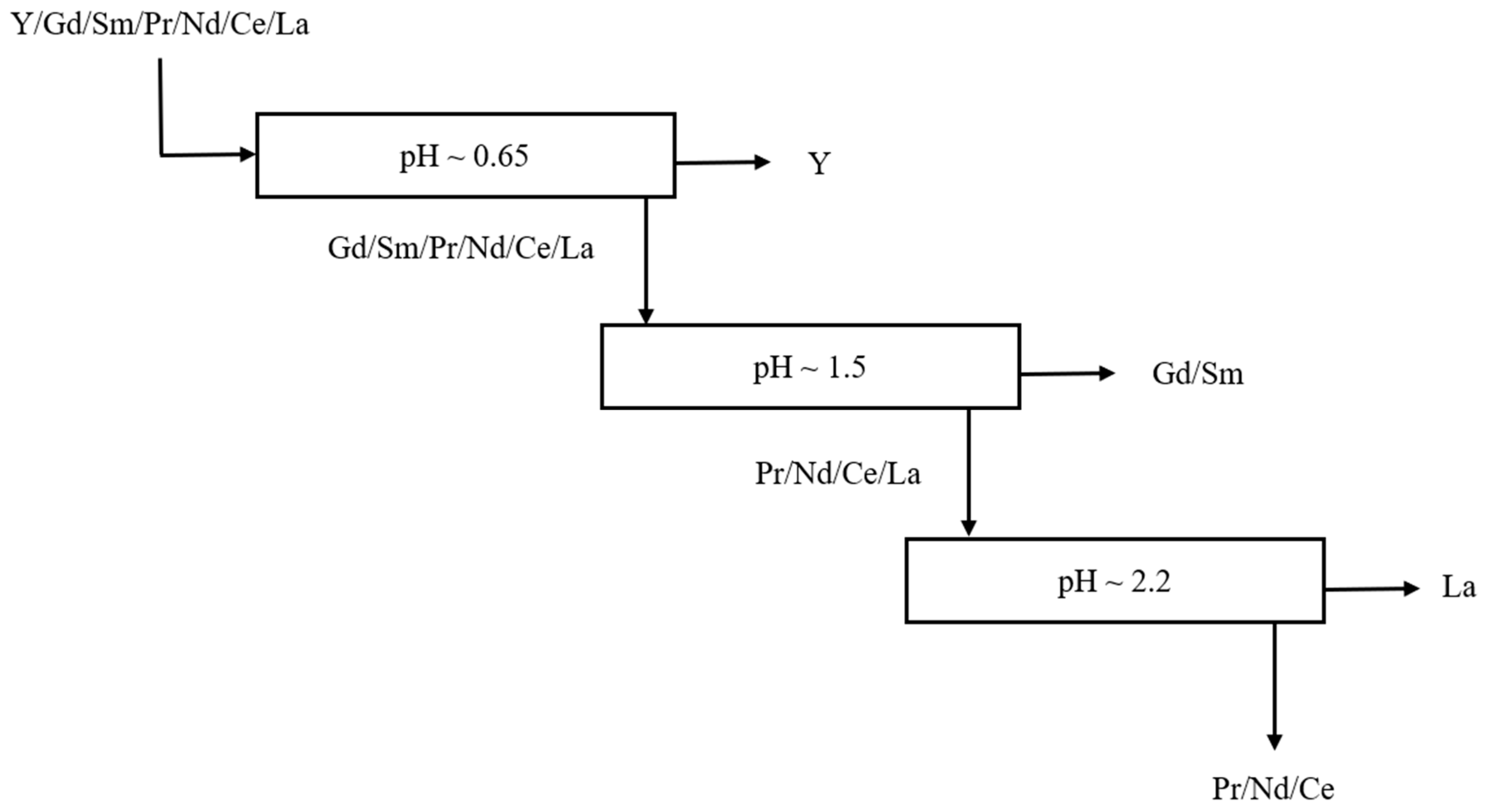
2.2. Part 2: Conceptual Flowsheet and pH Determination

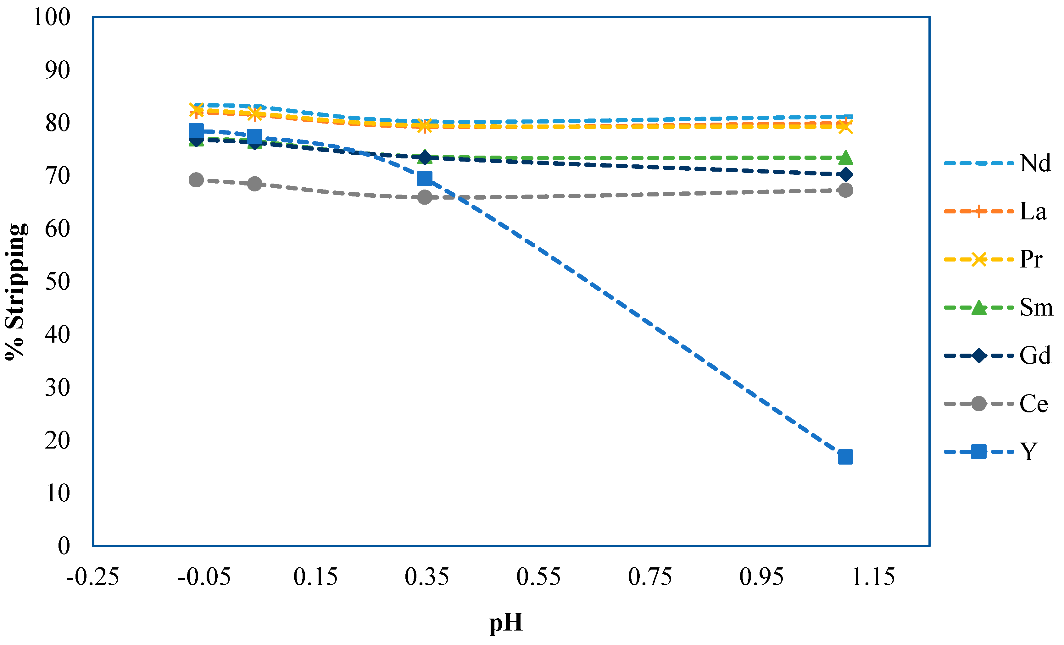
The feed material for the study was adapted from mixed rare earth oxide products produced as part of the research performed at the University of Kentucky to obtain REEs from coal sources [29,30]. Figure 9 shows the elemental distribution of the REEs of the concentrate produced, which had a total REE concentration of 44.05 ppm on analyzing 1 gm of oxide, and Figure 10 shows the selected distribution for test work on a total REE concentration of 10 gm/L. The justification for the simplification of the feed to the model solution was to reduce the complexity of the model demonstration by removing elements present in very small concentrations (less than 1 percent).

pH Selection

To determine the most favorable pH for separation of the elements, a preliminary modeling study performed previously [31] on the SX train shown in Figure 1 was conducted by developing a single variable pH model from extraction and stripping experiments. A pH sensitivity study was conducted on the train where pH was varied, and the concentration of strip bleed was observed. The pH resulting in high separation was selected. This approach would consider the effect of feed concentration changes in loading due to recirculating (reflux) streams from scrubbing and stripping. The results of these experiments are briefly described for convenience and serve as the base pH for the phase ratio experiments. This initial work was utilized in identifying specific separation pH values for elements and designing a preliminary SX flowsheet. Figure 11 shows results from extraction isotherms conducted on a mixed REE salt system in chloride media using a 5% DEHPA and 10% TBP mixture in Orfom (diluent) corresponding to 0.15 M and 0.36 M of DEHPA and TBP concentration, respectively. The concentration was selected to have an excess of extractant available for loading a high concentration of REEs determined after test work done at 1% and 2% DEHPA with 10% TBP mixture. Similarly, stripping experiments on organic loaded with REEs utilizing the same feed at a pH of 2.7 were also performed using hydrochloric acid 1 M to 6 M. Figure 12 shows stripping characteristics with equilibrium pH.

From the models in the initial studies [31], it was determined that a pH of 0.65 resulted in a high purity of Y in the stripped solution for the feed mixture, whereas a pH of 1.5 can be used in combined extraction of Gd and Sm and pH 2.2 resulted in high purity of La. Using the observation, a starting point is proposed involving three SX trains with different loading pH to separate elements (Figure 13).

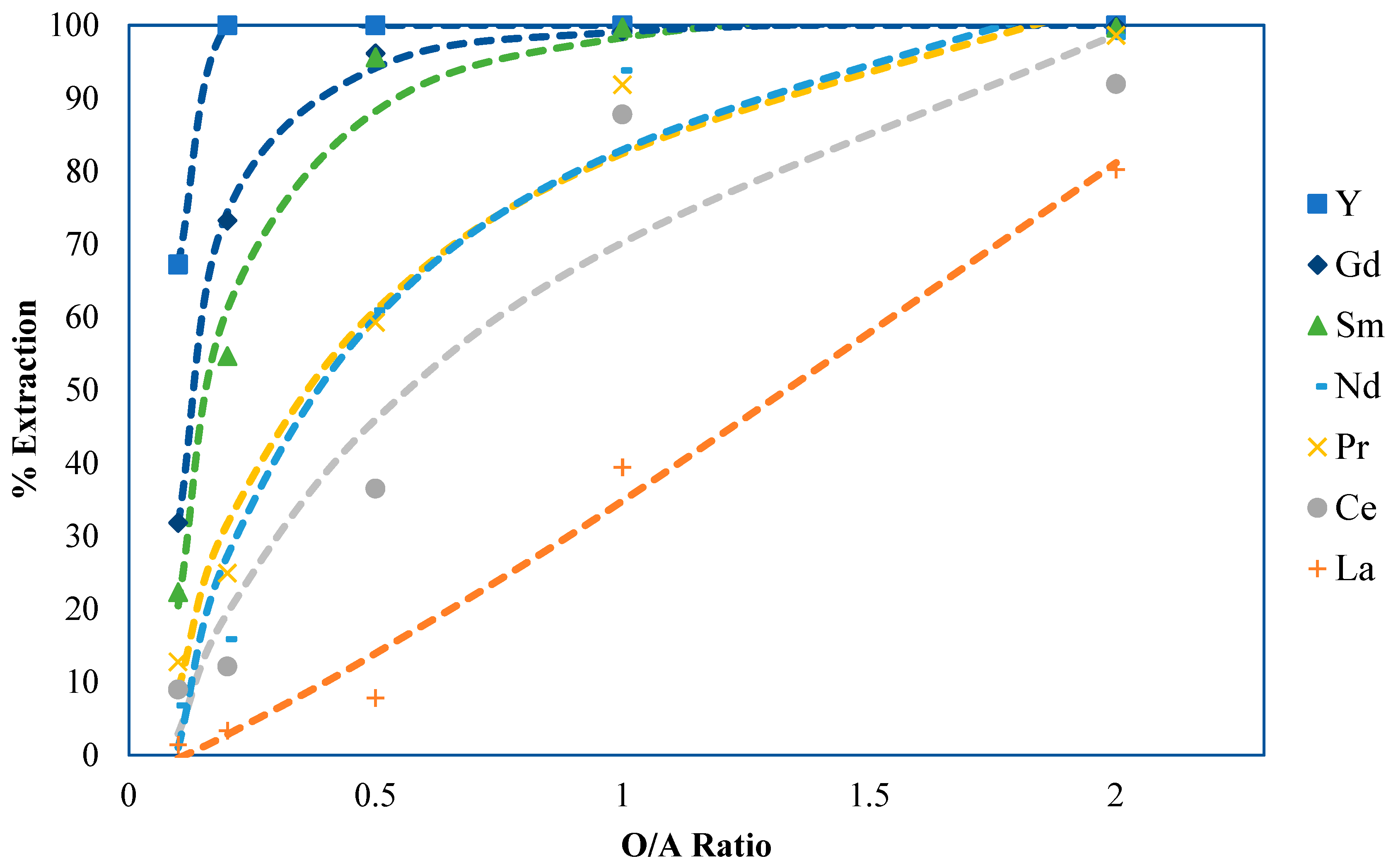
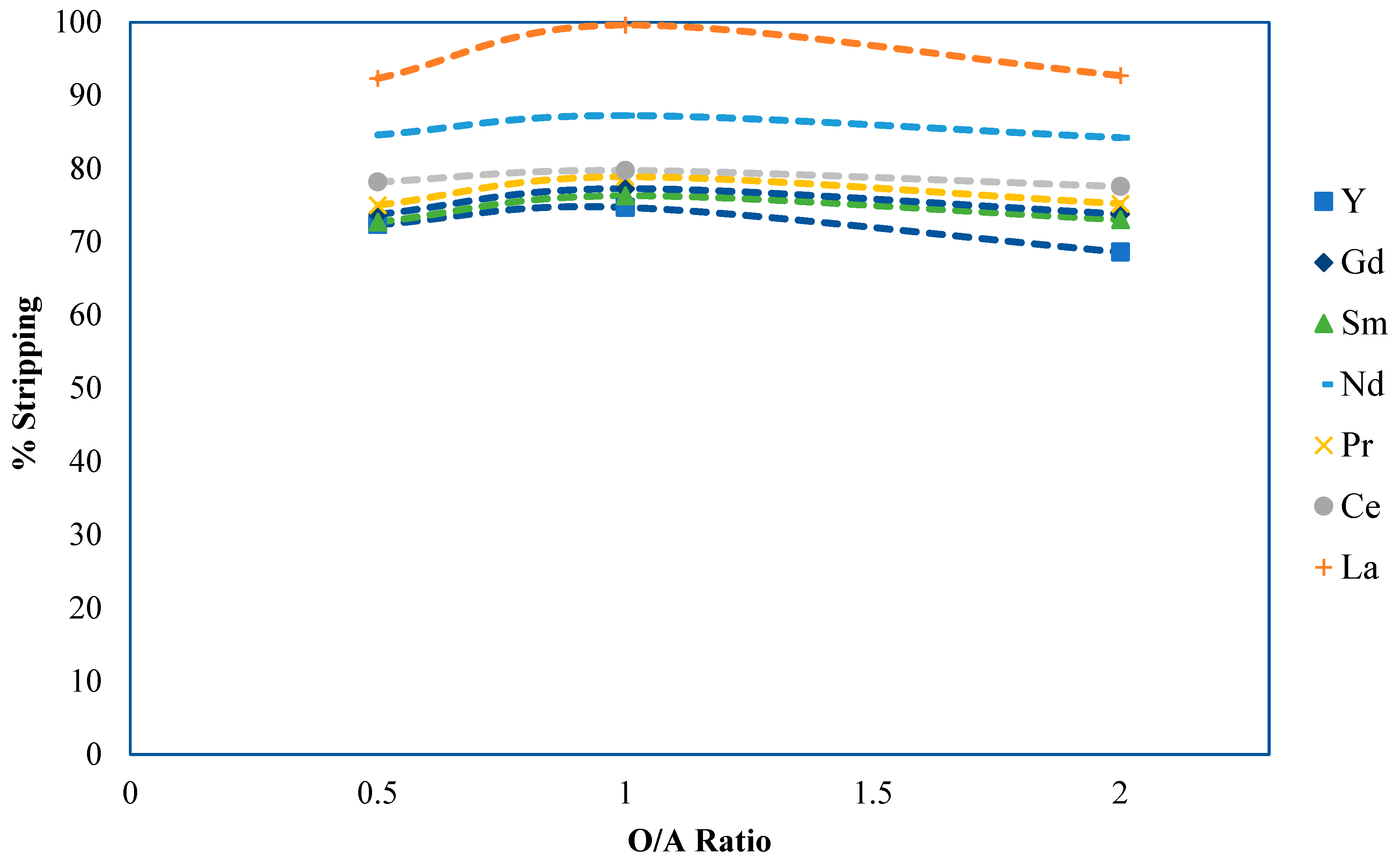
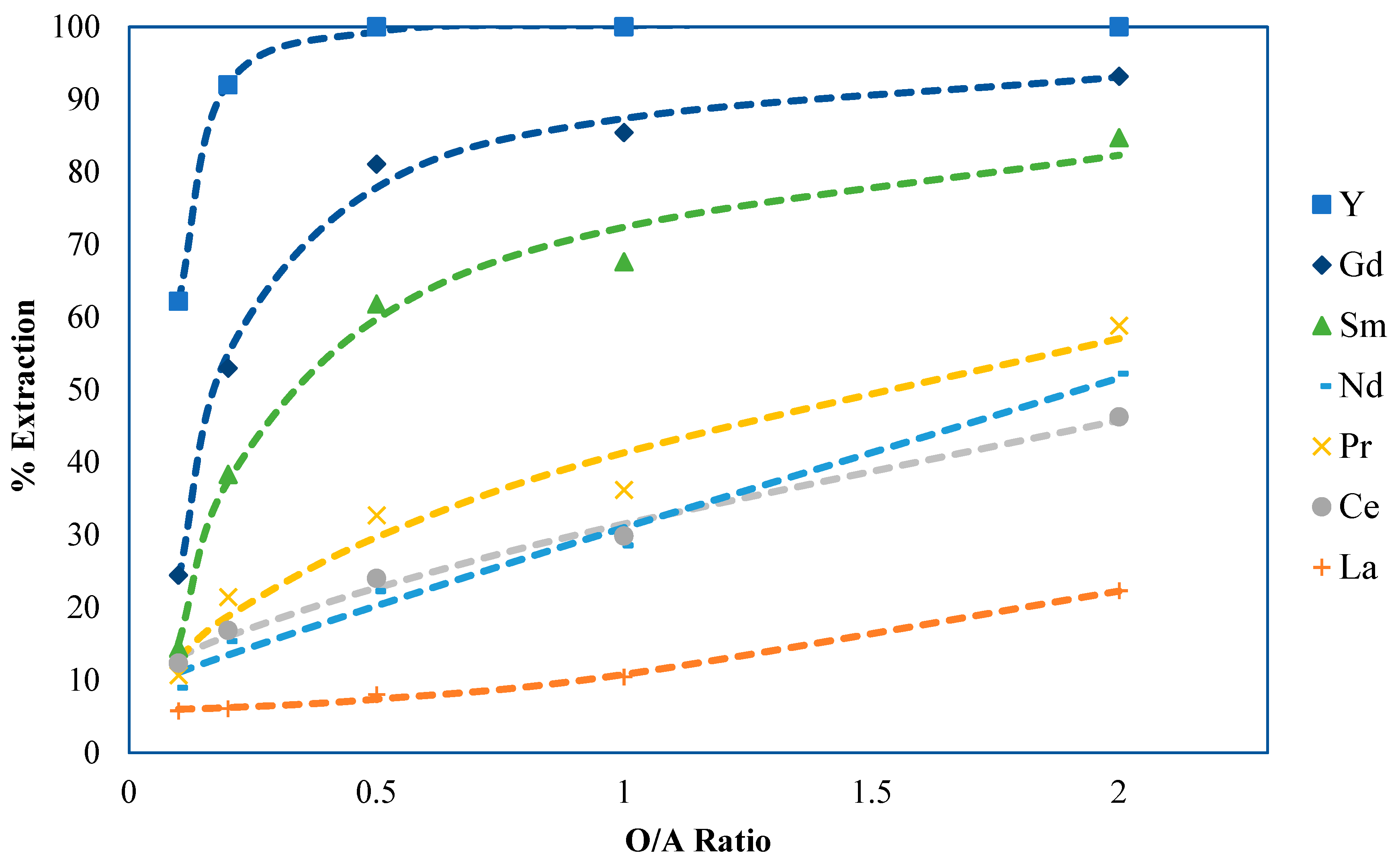
2.3. Part 3: Phase Ratio Determination and Extraction Equilibrium Development

2.3.1. Phase Ratio Development Methods and Materials

Based on Figure 13, the next step was to understand the effect of phase ratios on REE extraction, which are critical in determining stage combinations for an SX train. For this work, the effect of phase ratio was studied on identical mixed rare earth salts described in the previous section. The solution was prepared in a hydrochloric acid media, and rare earth salts used to prepare the mixture were obtained from Fisher Scientific, having a purity greater than 99 percent. The salts used were the oxides of lanthanum (La₂O₃), neodymium (Nd₂O₃), samarium (Sm₂O₃), gadolinium (Gd₂O₃), yttrium (Y₂O₃), hydrated chloride of cerium (CeCl₃·7H₂O), and praseodymium (PrCl₃). The chlorides of cerium (Ce) and praseodymium (Pr) used as their oxides are insoluble. For the organic phase, DEHPA (Di-2-ethylhexyl phosphoric acid) was used as the primary extractant, Orfom, which is a less aromatic non-carcinogenic derivative of kerosene, was used as the diluent, and TBP (Tributyl phosphate) as the phase modifier. DEHPA and Orfom were acquired from Cytec Canada Inc. (Niagara Falls, ON, Canada), and TBP was obtained from Beantown Chemicals. Analytical grade hydrochloric acid (HCl; 37% w/w), along with distilled water having a conductivity of 18 M ohms, was utilized to prepare the mixed rare earth salt solution. The molar solution of HCl prepared from its analytical grade and the molar solution of NaOH (sodium hydroxide) were used for adjusting the pH of the solution. Orion™ ROSS Ultra™ pH Electrode was used to measure the pH of the aqueous phase.

Extraction—The aqueous phase for the extraction experiment was prepared by taking a mixture of the aforementioned REE salts in a distribution shown in Figure 10 to add up to a total solid weight of 10 gm and dissolving it in 1 M of HCl acid to a volume of 1 L. The organic phase consisted of 50 mL of DEHPA (5% v/v) and 100 mL TBP (10% v/v) dissolved in Orfom to a total volume of 1 L to make up a concentration of 0.15 M and 0.36 M of DEHPA and TBP, respectively. The extraction experiments were then performed by taking 50 mL of the aqueous phase and equilibrating it with 5, 10, 25, 50, and 100 mL of the organic phase, respectively, to achieve the phase ratio of 1/10, 1/5, 1/2,1/1, and 2/1. Mixing was done in a conical flask using an agitator for 15 min. Post-mixing, the mixtures were allowed to stand for 20 min in a separatory funnel for phase disengagement. The pH of the aqueous phase was measured, compared, and readjusted to the target equilibrium pH shown in

Table 2. Target and measured pH for phase ratio experiments for all phase ratios (sample size of 5).

Targeted Equilibrium pH	Average Equilibrium pH Measured	Standard Deviation in Measured pH
0.65	0.659	0.003
1.5	1.523	0.014
2.2	2.234	0.028

. The process was repeated until the target equilibrium pH was reached. The aqueous samples were then analyzed for REE concentrations using ICP-OES. The standard samples of concentrations, 0.05, 0.5, 1, 5, and 10 ppm, were prepared for calibrating the ICP. A VHG element calibration standard, containing elements in a concentration of 100 μg/L, was mixed in appropriate weight with 5% HNO₃, prepared to the aforementioned standards. Upon calibration, the samples to be measured were loaded for measurement under different dilutions, 10×, 100×, and 1000×, of the raw samples. The dilution was performed to ensure the measured sample’s elemental concentration was within the equipment’s calibration range. Upon analysis, the concentration of REEs in the organic phase was back-calculated using the following equation:

$${\mathrm{C}}_{\mathrm{o}}=\frac{{\mathrm{V}}_{\mathrm{a}\mathrm{q}}\left({\mathrm{C}}_{\mathrm{a}\mathrm{q},\mathrm{f}\mathrm{e}\mathrm{e}\mathrm{d}}-{\mathrm{C}}_{\mathrm{a}\mathrm{q},\mathrm{e}\mathrm{q}}\right)}{{\mathrm{V}}_{\mathrm{o}}}$$

(20)

where C_o is the concentration of metal in the organic phase, and C_aq,feed and C_aq,eq are the concentrations in the aqueous phase, measured before and after extraction, respectively. V_aq and V_o are the volume of aqueous and organic phases (in mL).

Stripping—For the stripping phase ratio experiments, a loaded organic phase was first prepared by equilibrating the aqueous phase with the organic phase at a phase ratio of 1 to 1 at a pH of 2.7. The pH of 2.7 was chosen to load and saturate the organic phase to the maximum possible extent, as shown in Figure 11. The loaded organic phase was then divided into three fractions of 50 mL, which was stripped with 1 M HCl acid at different volumetric ratios. Volumes of 25, 50, and 100 mL of 1 M HCl were used, and the target equilibrium pH was 0.15. The equilibrium pH for stripping phase ratio analysis was selected on the basis of stripping isotherm shown in Figure 12. Since the stripping characteristics for the elements were mostly constant except yttrium, the pH of 0.15 was selected to strip all the elements and hence was used in the phase ratio study. Once the target equilibrium pH was reached, the stripped solutions were analyzed for REE concentration using ICP-OES.

2.3.2. Experimental Results and Discussion

The results from the extraction phase ratio experiments performed at pH 0.65 indicated Y as the only metal extracted in appreciable quantities, whereas extraction of other elements was negligible (below the detection limit of ICP with minimum detection of 0.05 ppm) for all elements except for the case of Gd at O/A ratio of 2 where 8.7% extraction was observed. Figure 14 shows the plot percent extraction of Y at differing O/A ratios. Figure 14 shows that 100 percent extraction was not achieved, even at higher O/A ratios. For this reason, a multi-stage configuration should be utilized to recover the element by providing multiple equilibrations.

At pH 1.5, the extraction of other components (Gd, Sm, Nd, Pr, Ce, and La) present in the feed mixture increased, confirming the pH dependence of the extraction (see Figure 15). However, increasing phase ratios correspond to increased extraction of all REEs. Low phase ratios showed prominent extraction for Y, Gd, and Sm, whereas increasing the phase ratios improves the extraction of all elements. The differences between Gd and Sm from other elements at low phase ratios can be utilized in improving its separation from other elements for the proposed conceptual flowsheet (Figure 13), provided that Y has been removed.

Similarly, Figure 16 shows percent extraction as a function of the phase ratio at an equilibrium pH of 2.2. As expected, the extraction of all the elements increased with an elevation in the solution pH. Like the previous example, percent extraction differences were higher at low phase ratios, which narrowed as the phase ratio increased. The pH 2.2 is important for the separation of Nd, Pr, and Ce from La based on the conceptual flowsheet (Figure 13).

To assist in the selection of a suitable phase ratio for separation, separation factors defined as follows were evaluated between adjacent elements:

$${\mathrm{S}}_{\mathrm{A}/\mathrm{B}}=\frac{{\mathrm{E}}_{\mathrm{A}}}{{\mathrm{E}}_{\mathrm{B}}}$$

(21)

where E_A and E_B represent the percent extraction of elements A and B at a given phase ratio, and S_A/B represent the separation factor.

Table 3. Separation factor for REE pairs at different phase ratios and pH.

pH	O/A Ratio	Y/Gd	Gd/Sm	Sm/Nd	Nd/Pr	Pr/Ce	Ce/La
1.5	0.1	2.54	1.69	1.61	0.84	0.87	2.13
	0.2	1.74	1.38	2.49	0.72	1.27	2.76
	0.5	1.23	1.31	2.78	0.68	1.36	2.99
	1	1.17	1.26	2.37	0.79	1.21	2.85
	2	1.07	1.10	1.62	0.89	1.27	2.07
2.2	0.1	2.11	1.43	3.27	0.53	1.42	6.29
	0.2	1.36	1.34	3.43	0.64	2.05	3.59
	0.5	1.04	1.01	1.57	1.03	1.62	4.64
	1	1.01	0.99	1.06	1.02	1.05	2.22
	2	1.00	1.00	1.01	1.00	1.07	1.15

provides the list of separation factors evaluated between element pairs at various phase ratios and pH conditions. For a combined extraction of Gd-Sm from Nd and other low-extracting elements, the separation factor of Sm/Nd was examined because of their extraction order. Thus, one can see from Table 3 at pH 1.5 that the separation results at an O/A ratio of 0.5 are better for Gd-Sm from Nd. Similarly, for Nd/Ce/Pr separation from La, the phase ratio of 0.5 at pH 2.2 is the preferred condition. The phase ratio of 0.5 was selected over 0.1 at pH 2.2 to have sufficient volume of an organic phase to facilitate mixing, dispersion, and phase disengagement during the process. Thus, using the information from Table 3, phase ratio conditions for a conceptual flowsheet were obtained.

Finally, in the case of stripping, there was no significant variation observed in percent stripping with a change in the phase ratio. Figure 17 shows the plot of experimental data performed on the loaded organic phase at different O/A ratios.

2.3.3. Development of Continuous Mathematical Expressions of Equilibrium for Model Input

The percent extraction data shown previously in Figure 14, Figure 15 and Figure 16 were fitted using a non-linear power function that best described the extraction relationship with the O/A ratio determined by the goodness-of-fit (R²). The same approach was followed for stripping experimental results shown in Figure 17, which were described by linear regression. The method of non-linear least squares was used as a criterion to determine the goodness-of-fit and obtain the parameters for the best fit. The mathematical form of the model obtained was:

$${\mathrm{E}}_{\mathrm{i},\mathrm{p}\mathrm{H}}\left(\mathrm{x}\right)={{\mathrm{a}}_{\mathrm{i},\mathrm{p}\mathrm{H}}(\mathrm{x}}^{{\mathrm{b}}_{\mathrm{i},\mathrm{p}\mathrm{H}}})+{\mathrm{c}}_{\mathrm{i},\mathrm{p}\mathrm{H}}$$

(22)

$${\mathrm{S}}_{\mathrm{i},\mathrm{p}\mathrm{H}}\left(\mathrm{x}\right)={\mathrm{a}}_{\mathrm{i},\mathrm{p}\mathrm{H}}\left(\mathrm{x}\right)+{\mathrm{b}}_{\mathrm{i},\mathrm{p}\mathrm{H}}$$

(23)

where E_i.pH represents the percent extraction to the organic phase of metal, subscripts i metal species, x the organic–aqueous phase ratio at constant and specific equilibrium pH, and a_i, b_i, and c_i represent the model parameters at respective pH. The same convention follows for Equation (23), with S_i representing the percent stripping of metal.

Table 4. Summary of coefficient and R² for the fitted models.

Elements	a	b	c	R2	Equilibrium pH
Y	1141.29	0.02	−1068.81	0.993	0.65
Y	−0.23	−2.22	100.40	0.999	1.5
La	4.87	1.75	5.94	0.997
Ce	22.82	0.70	8.70	0.992
Pr	44.70	0.44	−3.36	0.961
Nd	22.57	0.94	8.46	0.983
Sm	−45.70	−0.35	118.10	0.989
Gd	−14.30	−0.74	101.67	0.994
Y	0.00	−15.07	100.00	1.000	2.2
La	37.94	1.15	−3.11	0.986
Ce	160.41	0.24	−90.20	0.917
Pr	−862.16	−0.04	944.61	0.971
Nd	−397.83	−0.08	480.77	0.956
Sm	−12.29	−0.87	110.61	0.975
Gd	−3.21	−1.34	102.30	0.998

summarizes the model parameters and R-squared values.

2.4. Part 4: Flowsheet Development and Optimization

The conceptual flowsheet shown in Figure 13 was developed using Simulink block models, and simulation was commenced by providing the separation conditions of the respective trains. For this work, the objective function and optimization were configured for each train and were performed sequentially, allowing a train-wise progression of optimization through the circuit. The pH condition described in the conceptual flowsheet (Figure 13) and phase ratio selected from Table 3 were used as settings to derive flow rates of the input streams for the simulation. SX train 1 was configured first to separate the Y based on the order of element extractability. The aqueous feed flow rate to loading stages was set to 0.9 lpm, stripping to 0.5 lpm with a reflux ratio of 0.2 in the scrubbing stages, resulting in a total flow rate of 1 lpm in the loading stage. This was performed to maintain a phase ratio of 1 in loading and 2 in stripping. At pH 0.65, an organic–aqueous flow ratio of 1 prevents the co-extraction of Gd during loading in the feed. Stripping is not significantly affected by variations in phase ratio (see Figure 17); hence, a phase ratio of 2 was set in stripping. A low-strip acid flow rate reduces the acid consumption cost and results in a concentrated bleed.

The total aqueous flow rate of 1 lpm in the loading stage was selected based on laboratory tests, which were performed using 10 gm of mixed salt in 1 L of solution in the loading process. The flow rates for organic and strip acid were derived using aqueous flow rate as the basis and selected phase ratio.

Table 5. Separation condition for yttrium used in SX-train-1.

Operating Parameters	Value
Feed flow rate (lpm)	0.9
Organic flow rate (lpm)	1
Strip flow rate (lpm)	0.5
Reflux ratio	0.2
Loading equilibrium pH	0.65
Strip equilibrium pH	0.15 (0.70 M)

lists the input conditions determined and used in the simulation. After confirming the input conditions, the SX train was ready for simulation to determine stage configuration. PSO was implemented across SX train 1, with loading (n_L), scrubbing (n_Sc), and stripping (n_St) stages as unknown variables. The parameters for the PSO listed in

Table 6. Particle swarm optimization parameters used during the simulation.

Condition	Value
Number of particles	10
Maximum iterations	20
w	0.8
c1	2
c2	2
Boundary conditions for stages	$1\le {\mathrm{n}}_{\mathrm{L}},{\mathrm{n}}_{\mathrm{S}\mathrm{c}},{\mathrm{n}}_{\mathrm{S}\mathrm{t}}\le 20$

were initialized, and the region for search space, also called boundary conditions, was defined.

The parameters of PSO were selected based on the understanding of the optimization method and the literature [28]. The knowledge used in the selection of parameters is:

(1) The number of particles and iterations: These are arbitrary and determined by the users based on the complexity of the problem, the dimensionality of the problem, the range of search space, and then monitoring the objective function value by multiple trials. The user balances the computational expense of more particles and iterations to insufficient investigation of the search space, leading to non-global optimums. The current case involves three dimensions (n_L, n_Sc, and n_St) with a small search space determined by the boundary stage conditions listed in Table 6; hence, 10 particles were selected with maximum iterations of 20. This allows 10 sets of stage combinations to search for optimum values at every iteration, as shown in Equation (24), thereby resulting in 200 unique opportunities to find an optimum. The columns in the matrix shown in Equation (24) indicate the stage number corresponding to n_L, n_Sc, and n_St (number of discrete variables for optimization), and the row indicates the number of particles. Thus, 10 rows and 3 columns signify 10 unique stage combinations varying three variables for an iteration. If the optimum value is unattained, the iterations can be increased;

$$\overrightarrow{P}={\left[\begin{array}{ccc}17& \cdots & 4\\ ⋮& \ddots & ⋮\\ 3& \cdots & 12\end{array}\right]}_{10\times 3}$$

(24)

(2) Inertia weight and acceleration coefficients: Inertia weight is a factor (w) in the velocity correction (Equation (13)), which determines the weightage given velocity (change in number of stages) from the previous iteration. It serves as a memory of particles during the update at the next iteration, generally taken as 0.8. Acceleration coefficients c₁ and c₂ in Equation (13), on the other hand, represent the velocity correction weightage towards particle local optimum or swarm global optimum. Both the variables can be tuned based on the problem; however, in general, it is suggested that c₁ and c₂ be set at 2 [29]. In the case of SX-train optimization, the inertia associated with velocity modifies the rate of change of the number of stages (n_L, n_Sc, and n_St). Similarly, c₁ and c₂ signify the “acceleration coefficient” for the number of stages (n_L, n_Sc, and n_St) based on the particle’s identified best position (particle’s stage combination leading to best purity) and the group-identified best position (group’s stage combination leading to best purity);

(3) Variable boundary conditions: The boundary condition essentially defines the search space, which is based on the problem being solved. For a stage determination problem, a minimum of 1 stage is needed in the loading, scrubbing, and stripping processes, which is established via a lower range of variables. The upper range of 10 was initially selected for trains, which resulted in 10 loading, scrubbing, and stripping stages, respectively. If the objective of the SX train was not met, the upper range was updated by 10 more stages. However, there is a possibility that updating the stage number does not result in any change in the objective function value, implying a separation problem.

After defining the PSO parameters, the train was simulated and optimized for stage number, resulting in a minimum value of the objective function described by Equation (17). Recovery of 99.61 and purity of 99.52 were obtained for yttrium extraction in the strip bleed, using an 8-12-3 stage combination of loading, scrubbing, and stripping, respectively. Figure 18 shows a convergence plot for SX-train-1, showing error minimization by PSO iteration. Figure 19 shows the recovery, purity, and concentration values for the elements in the input and output streams. It was observed that a large number of scrubbing stages are critical for achieving high purity. The strip bleed can be further purified by adding an additional cleaner SX train for the bleed and employing the same method. However, in this case, additional purification was not required. The obtained stage combination was updated in SX train 1, and the flowsheet design progressed to the next SX train for a combined separation of Gd and Sm from the raffinate in SX train 1. The parameter associated with the next stage objective function was the stage combination of the respective train, whereas the optimization parameters were kept the same as listed in Table 6. This approach of a piecewise optimization of the SX train was adopted because the objective of each SX train proposed in the conceptual flowsheet was different. Each train is intended to separate a particular element or element combination with the objectives of maximizing recovery and purity described by Equation (17). However, when the combined objective function was not useful in separation, the purity function described by Equation (18) was used.

2.4.1. Gadolinium and Samarium Separation

The raffinate from SX train 1, having a minor concentration of Y of 0.21 ppm, was processed in SX train 2 for a combined extraction of Gd and Sm. Following the same approach, train 2 was simulated iteratively to identify stage combinations, using the optimization algorithm to maximize recovery and purity. It was found that the best value attained by the objective function was 41.08 for a 10-3-1 stage combination. The stage combination resulted in high Gd and Sm recovery with values greater than 99 percent; however, the purity was significantly lower, with values of 11.20 and 9.71 percent, respectively. The reason for such a low purity value is that the concentration of Gd and Sm in the feed is much smaller than Nd and Ce, which, despite having a low percent of extraction, are recovered in higher concentrations.

Thus, the combined separation of both elements from the raffinate mixture by maximizing both recovery and purity is not advantageous. For the following reason, it was sought to maximize the combined purity of the Gd and Sm in the strip bleed stream. This was done using the purity of Sm as the objective function given by Equation (18). The reason only the purity of Sm is considered in the objective function and not of Gd is because of the order of extraction of elements. Setting the objective function as the purity of Sm will automatically maximize Gd because it is being extracted before Sm. Nevertheless, the objective function was switched to account for the purity of Sm to achieve a lower concentration of the undesired element (Nd, Pr, Ce, and La) in the strip bleed. This resulted in the combined purity of 80.65% in the strip bleed for Gd and Sm and the remaining 19.34% of Nd, Pr, Ce, and La. Figure 18 shows the convergence plot for maximizing the purity of Sm in the strip bleed stream. The recovery of Gd and Sm in the strip bleed was 25.48 and 22.11, respectively, and in the raffinate, it was 13.62 and 0.23 percent, respectively, indicating a majority of the pair associated with the extractant in the organic stream.

The strip bleed was further processed by an additional SX train 3 to seek potential separation between Gd and Sm, using the purity of Gd in the strip bleed as the objective. The best performance resulted in a purity of 72.59 for Gd and Sm 22.25, indicating the difficult separation of the pair. The raffinate from SX-train-2, rich in Nd, Pr, Ce, and La, was sent for further processing to SX-train 4, while the raffinate from SX-train-3 was left untreated, but it can be recycled to train 1 to prevent any loss.

2.4.2. Lanthanum Separation

The raffinate stream from SX train 2 was processed to further separate La from the element mixture consisting of Nd, Pr, Ce, and La. It was performed by extracting Nd, Pr, and Ce in the strip bleed and leaving the La in the raffinate stream using SX train 4 (Figure 19). The reason this approach was adopted is due to La having a low percentage of extraction compared to other elements, as shown in Figure 16, and the ease of extraction of Nd, Pr, and Ce to the organic phase, leaving La in the raffinate. The purity of Ce in the strip bleed was used as the objective function. A 10-3-5 stage combination of loading, scrubbing, and stripping, respectively, yielded a purity of 85.41 percent La in the raffinate stream, with the only other major component as Ce with 14.23 percent at a phase ratio of 0.5 in the loading stage. Higher purity La can be achieved if the phase ratio of 0.1 is maintained in the loading stage of train 4, as the separation factor is highest, having a value of 6.29, as listed in Table 3. The strip bleed resulting from train 4 still contained a considerable amount of La, which could be further processed to recover La. Nevertheless, using the block model and PSO method, the stage combination for the separation of mixed REEs was determined.

Table 7. Summary of the train optimization objective function and results.

Train	Objective Function	Element Separated	Purity	Stage Combination (Loading–Scrubbing–Stripping)
Train-1	Recovery and Purity of Y	Y	99.52	8-12-3
Train-2	Purity of Sm	Gd-Sm combined	46.00/34.65 (80.65)	7-9-6
Train-3	Purity of Gd	Gd/Sm	72.59	14-8-5
Train-4	Purity of Ce	Nd, Pr, Ce combined/La	26.74/7.94/54.60 (89.28)	10-3-5

summarizes the element separation objective function associated with individual SX trains along with the determined stage combination and purities obtained.

3. Conclusions

Flowsheet development for individual and group separation of the REEs from a mixture via a combined equilibrium and process modeling approach using a roughing SX process was described in this paper. Experiments at different phase ratios at pre-determined pH of 065, 1.5, and 2.2 were conducted to study changes in the equilibrium separation characteristics of the elements. Experimental results indicated an increase in the extraction performance of the REEs with an increase in phase ratio; however, the stripping characteristics were generally constant with varying phase ratios. The phase ratio results were used to identify separation conditions of the previously proposed conceptual flowsheet using separation factors as criteria and develop the equilibrium phase ratio models. Organic to aqueous (O/A) phase ratios of 1/1, 1/2, and 1/2 were selected for the separation of Y, Gd-Sm, and La from the feed mixture for loading, and a phase ratio of 2/1 was selected for the stripping process.

Function block models were developed in Simulink by integrating equilibrium phase ratio models in a process modeling framework to predict stagewise mass transfer for a multi-component system. With the aid of block models and the application of particle swarm optimization, the conceptual flowsheet was designed and simulated to determine the stage combination, resulting in the optimum separation of elements using purity, recovery, or both as the objective function. The optimization results indicated effective separation of yttrium and lanthanum from the feed mixture at 99.52 and 85.41 percent, respectively, whereas separation of other elements was also possible to a lesser extent. Stage combinations of 8-12-3 and 10-3-5 in loading, scrubbing, and stripping were estimated by PSO for the aforementioned product purities. Various stage combinations were tested by the optimization algorithm to yield better separability with recovery and purity for Gd-Sm and Nd-Pr-Ce element groups. However, the individual separation for the groups was difficult, irrespective of separation condition and stage combination. It was also observed that a large number of scrubbing stages are essential in obtaining high-purity products. The combined equilibrium and process modeling approach presented in this work can be used to design and simulate SX flowsheets of any configuration. The block model developed in Simulink provides the ability to analyze separation performance with respect to different process variables. The method presented is anticipated to provide a convenient way to analyze multi-component systems for any feed mixture and extractant combination, provided bench-scale equilibrium test results are available. It also provides an opportunity for future researchers to develop a library of different reagent schemes and equilibrium models, perform sensitivity analysis for different process variables, and develop an economic analysis module, which would enhance the application of the tool.

References

1. Du, X.; Graedel, T.E. Global rare earth in-use stocks in NdFeB permanent magnets. J. Ind. Ecol. 2011, 15, 836–843. [Google Scholar] [CrossRef]
2. Ganguli, R.; Cook, D.R. Rare earths: A review of the landscape. MRS Energy Sustain. 2018, 5, E9. [Google Scholar] [CrossRef]
3. Pavel, C.C.; Lacal-Arantegui, R.; Marmier, A.; Schuler, D.; Tzimas, E.; Buchert, M.; Jenseit, W.; Blagoeva, D. Substitution strategies for reducing the use of rare earths in wind turbines. Resour. Policy 2017, 52, 349–357. [Google Scholar] [CrossRef]
4. Schmid, M. Mitigating supply risks through involvement in rare earth projects: Japan’s strategies and what the US can learn. Resour. Policy 2019, 63, 101457. [Google Scholar] [CrossRef]
5. Xie, F.; Zhang, T.A.; Dreisinger, D.; Doyle, F. A critical review on solvent extraction of rare earths from aqueous solutions. Miner. Eng. 2014, 56, 10–28. [Google Scholar] [CrossRef]
6. Jha, M.K.; Kumari, A.; Panda, R.; Kumar, J.R.; Yoo, K.; Lee, J.Y. Review on hydrometallurgical recovery of rare earth metals. Hydrometallurgy 2016, 165, 2–26. [Google Scholar] [CrossRef]
7. Rydberg, J. Solvent Extraction Principles and Practice, Revised and Expanded; CRC Press: New York, NY, USA, 2004. [Google Scholar]
8. Turgeon, K.; Boulanger, J.-F.; Bazin, C. Simulation of Solvent Extraction Circuits for the Separation of Rare Earth Elements. Minerals 2023, 13, 714. [Google Scholar] [CrossRef]
9. Mohammadi, M.; Forsberg, K.; Kloo, L.; de la Cruz, J.M.; Rasmuson, Å. Separation of Nd (III), Dy (III) and Y (III) by solvent extraction using D2EHPA and EHEHPA. Hydrometallurgy 2015, 156, 215–224. [Google Scholar] [CrossRef]
10. Basualto, C.; Valenzuela, F.; Molina, L.; Munoz, J.; Fuentes, E.; Sapag, J. Study of the solvent extraction of the lighter lanthanide metal ions by means of organophosphorus extractants. J. Chil. Chem. Soc. 2013, 58, 1785–1789. [Google Scholar] [CrossRef]
11. Free, M. Hydrometallurgy: Fundamentals and Applications; John Wiley & Sons: Hoboken, NJ, USA, 2013. [Google Scholar]
12. Zhang, J.; Zhao, B.; Schreiner, B. Separation Hydrometallurgy of Rare Earth Elements; Springer: Cham, Switzerland, 2016. [Google Scholar]
13. Thakur, N. Separation of rare earths by solvent extraction. Miner. Process. Extr. Metullargy Rev. 2000, 21, 277–306. [Google Scholar] [CrossRef]
14. Anitha, M.; Singh, H. Artificial neural network simulation of rare earths solvent extraction equilibrium data. Desalination 2008, 232, 59–70. [Google Scholar] [CrossRef]
15. Giles, A.; Aldrich, C. Modelling of rare earth solvent extraction with artificial neural nets. Hydrometallurgy 1996, 43, 241–255. [Google Scholar] [CrossRef]
16. Sharp, B.M.; Smutz, M. Stagewise Calculation for Solvent Extraction System Monazite Rare Earth Nitrates-Nitric Acid-Tributyl Phosphate-Water. Ind. Eng. Chem. Process. Des. Dev. 1965, 4, 49–54. [Google Scholar] [CrossRef]
17. Sebenik, R.F.; Sharp, B.M.; Smutz, M. Computer Solution of Solvent-Extraction-Cascade Calculations for the Monazite Rare-Earth Nitrates-Nitric Acid-Tributyl Phosphate-Water System. Sep. Sci. 1966, 1, 375–386. [Google Scholar] [CrossRef]
18. Voit, D.O. Computer simulation of rare earth solvent extraction circuits. In Rare Earths, Extraction, Preparation and Applications; The Minerals, Metals & Materials Society: Pittsburgh, PA, USA, 1988; pp. 213–226. [Google Scholar]
19. Reddy, M.L.P.; Ramamohan, T.; Bhat, C.C.S.; Shanthi, P.; Damodaran, A. Mathematical Modelling of the Liquid-Liquid Extraction Separation of Rare Earths. Miner. Process. Extr. Metall. Rev. 1992, 9, 273–282. [Google Scholar] [CrossRef]
20. Wenli, L.; D’Ascenzo, G.; Curini, E.; Chunhua, Y.; Jianfang, W.; Tao, J.J.; Minwen, W. Simulation of the development automatization control system for rare earth extraction process: Combination of ESRECE simulation software and EDXRF analysis technique. Anal. Chim. Acta 2000, 417, 111–118. [Google Scholar] [CrossRef]
21. Bourget, C.; Soderstrom, M.; Jakovljevic, B.; Morrison, J. Optimization of the Design Parameters of a CYANEX® 272 Circuit for Recovery of Nickel and Cobalt. Solvent Extr. Ion Exch. 2011, 29, 823–836. [Google Scholar] [CrossRef]
22. Soderstrom, M.; Bourget, C.; Jakovljevic, B.; Bednarski, T. Development of process modeling for CYANEX® 272. In ALTA 2010 Nickel/Cobalt, Copper and Uranium Proceedings; ALTA Metallurgical Services: Melbourne, Australia, 2010; pp. 1–17. [Google Scholar]
23. Evans, H.A.; Bahri, P.A.; Vu, L.T.; Barnard, K.R. Modelling cobalt solvent extraction using Aspen Custom Modeler. In Computer Aided Chemical Engineering; Klemeš, P.S.V.J.J., Liew, P.Y., Eds.; Elsevier: Amsterdam, The Netherlands, 2014; Volume 33, pp. 505–510. [Google Scholar]
24. Lyon, K.; Greenhalgh, M.; Herbst, R.S.; Garn, T.; Welty, A.; Soderstrom, M.D.; Jakovljevic, B. Enhanced Separation of Rare Earth Elements. 2016. Available online: https://www.osti.gov/biblio/1363891 (accessed on 1 September 2016).
25. Liu, Y.; Spencer, S. Dynamic simulation of grinding circuits. Miner. Eng. 2004, 17, 1189–1198. [Google Scholar] [CrossRef]
26. Srivastava, V.K. Modeling of Rare Earth Solvent Extraction Process for Flowsheet Design and Optimization. Ph.D. Thesis, University of Kentucky, Lexington, KY, USA, 2021. Volume 62. [Google Scholar]
27. Kennedy, J.; Eberhart, R. Particle swarm optimization. In Proceedings of the ICNN’95-International Conference on Neural Networks, Perth, WA, Australia, 27 November–1 December 1995; IEEE: New York, NY, USA, 1995; Volume 4, pp. 1942–1948. [Google Scholar]
28. He, Y.; Ma, W.J.; Zhang, J.P. The parameters selection of PSO algorithm influencing on performance of fault diagnosis. In Proceedings of the MATEC Web of Conferences, Cape Town, South Africa, 1–3 February 2016. [Google Scholar]
29. Honaker, R.; Zhang, W.; Yang, X.; Rezaee, M. Conception of an integrated flowsheet for rare earth elements recovery from coal coarse refuse. Miner. Eng. 2018, 122, 233–240. [Google Scholar] [CrossRef]
30. Zhang, W.; Honaker, R. Process development for the recovery of rare earth elements and critical metals from an acid mine leachate. Miner. Eng. 2020, 153, 106382. [Google Scholar] [CrossRef]
31. Srivastava, V.; Werner, J. Solvent Extraction Flowsheet Design for the Separation of Rare Earth Elements: Tools, Methods and Application. In Proceedings of the Conference of Metallurgists, COM 2020, Virtual Event, 14–15 October 2020. [Google Scholar]
Figure 1. Multi-stage SX process (top, adapted from [5]); mass balance across a single stage showing flow and concentration variables associated with a single stage (middle) and multi-stage SX process involving loading, scrubbing, and stripping with reflux (bottom).
Mining 03 00031 g001
Figure 2. Cause and effect diagram showing factors influencing SX performance.
Mining 03 00031 g002
Figure 3. Loading and stripping from a single stage.
Mining 03 00031 g003
Figure 4. Extraction and stripping from multi-stage loading and stripping process.
Mining 03 00031 g004
Figure 5. Working of a Simulink system block.
Mining 03 00031 g005
Figure 6. Solvent extraction model library developed in Simulink.
Mining 03 00031 g006
Figure 7. Interconnected subsystem of loading, scrubbing, and stripping process to develop SX train block.
Mining 03 00031 g007
Figure 8. SX flowsheet developed using Simulink block models for Y separation.
Mining 03 00031 g008
Figure 9. REE distribution of the mixed oxide product recovered from West Kentucky No. 13 (Baker) seam coarse refuse.
Mining 03 00031 g009
Figure 10. Reconstituted REE distribution of the mixed oxide product recovered from West Kentucky No. 13 (Baker) seam coarse refuse, omitting REEs of less than 1%.
Mining 03 00031 g010
Figure 11. Equilibrium isotherm for loading showing percent extraction of REEs at different pHs and phase ratio 1 using a 5% DEHPA and 10% TBP mixture in Orfom (diluent).
Mining 03 00031 g011
Figure 12. Equilibrium isotherm for scrubbing and stripping at a phase ratio of 1 performed using HCl on organic solution loaded to pH 2.7.
Mining 03 00031 g012
Figure 13. Conceptual flowsheet for separation of REEs based on pH study.
Mining 03 00031 g013
Figure 14. Percent extraction vs. O/A ratio at pH 0.65. Note that other elements are not included due to lack of extraction.
Mining 03 00031 g014
Figure 15. Percent extraction vs. O/A ratio at pH 1.5.
Mining 03 00031 g015
Figure 16. Percent extraction vs. O/A ratio at pH 2.2.
Mining 03 00031 g016
Figure 17. Percent stripping vs. O/A ratio using 1 M HCl.
Mining 03 00031 g017
Figure 18. Convergence plot for Train 1, Train 2, and Train 3 (optimized independently and plotted together) showing the minimization of the objective function with iteration.
Mining 03 00031 g018
Figure 19. Simulated and optimized flowsheet showing stage number, concentration, and purity level.
Mining 03 00031 g019