GPU-Enabled Volume Renderer for Use with MATLAB

Abstract

Traditional tools, such as 3D Slicer, Fiji, and MATLAB^®, often encounter limitations in rendering performance and data management as the dataset sizes increase. This work presents a GPU-enabled volume renderer with a MATLAB^® interface that addresses these issues. The proposed renderer uses flexible memory management and leverages the GPU texture-mapping features of NVIDIA devices. It transfers data between the CPU and the GPU only in the case of a data change between renderings, and uses texture memory to make use of specific hardware benefits of the GPU and improve the quality. A case study using the ViBE-Z zebrafish larval dataset demonstrated the renderer’s ability to produce visualizations while managing extensive data effectively within the MATLAB^® environment. The renderer is available as open-source software.

1. Introduction

The visualization of volumetric data is an important task, especially in medical and biomedical applications [1]. Various image acquisition techniques, such as fMRI and 3D microscopy, are used to generate volumetric datasets. These visualizations play a crucial role not only in everyday medical practice, such as preparing for and following up on surgical interventions, but also in educational contexts, including publications, textbooks, and research analysis [2,3,4,5,6]. Beyond static images, dynamic visualizations, such as videos, provide additional insights. A notable example is the visualization of a whole-brain MRI [7]. Moreover, a 3D digital anatomy model has proven invaluable in improving communication and fostering a better understanding between physicians and patients [8].

Prominent visualization tools used in research include 3D Slicer [9] and Fiji [10], along with plugins, such as ClearVolume [11], which provide interactive 3D microscopy capabilities. Immersive platforms, such as the iDaVIE framework, further enhance the interpretability of complex datasets by enabling researchers to render and explore 3D volumetric data from modalities like MRI and microscopy in virtual reality environments [12]. In pediatric echocardiography, stereoscopic visualization has been extended to platforms such as Microsoft HoloLens, allowing for immersive, real-time diagnostic exploration [13].

The demand for high-quality, interactive visualizations continues to grow as volumetric datasets increase in size and complexity. Computational efficiency becomes a critical factor, as rendering large datasets requires robust memory management and hardware optimization. The techniques for optimizing data transfer between the host and the device, such as those proposed by Fujii et al. [14], underscore the importance of reducing the memory transaction overhead in GPU-accelerated rendering. Recent work by Gao et al. [15] introduced optimized GPU memory strategies for managing mesh-rendering processes in monocular 3D reconstruction, offering a modern approach to improving rendering pipelines for large datasets. Furthermore, machine learning methods, such as uncertainty-aware neural radiance fields, offer innovative solutions to streamline rendering processes, enabling single-view reconstructions and optimized workflows for volumetric medical imaging [16].

MATLAB^® is a prominent tool for 3D image analysis within the scientific community [17,18]. It supports a variety of extensions and modules, such as VoxelStats [19] for voxel-wise brain analysis and Hydra [20], a GPU-based image analysis library. MATLAB^®’s built-in tool Medical Image Labeler [21], introduced in R2022b, allows for comprehensive workflows for image annotation, segmentation, and visualization. The integration of tools like the Volume Viewer App [22], VolumeRender [23], and Ray Tracing Volume Renderer [24] expands MATLAB^®’s functionality for volumetric rendering. However, while these tools offer visualization capabilities and some degree of customization, they often lack fully programmable rendering features, such as customizable lighting, material properties, and camera controls.

To address the limitations of existing MATLAB^® solutions, this work presents a novel GPU-enabled rendering system featuring fully adjustable emission, absorption, and reflection properties, along with a configurable illumination setup. Our system supports the modification of camera parameters to create animations, stereo images for 3D displays, and anaglyph images for viewing with standard red–cyan glasses, ensuring accessibility to a wider audience. To ensure high usability for end users, a MATLAB^® interface was developed to interact with the rendering engine, which was implemented in C++ and CUDA. These capabilities enable the creation of complex, high-quality renderings while leveraging the parallelization potential of modern GPUs, allowing scientists to utilize MATLAB^® as a comprehensive tool for analysis and visualization, thereby enabling workflows within a single environment.

1.1. Rendering Equation

There are two prominent classes of methods used to render a volume: indirect and direct volume rendering (see Figure 17 in [25]). Indirect volume rendering involves creating intermediate representations from volumetric data before rendering. One example of indirect rendering is to render the isosurface of a volume [26]. First, the generation of an intermediate representation of the dataset is required (e.g., a polygonal representation of an isosurface generated by Marching Cubes [27]). The second step is the rendering of this representation. In such a polygonal representation, potentially only a limited number of voxels in the 3D dataset directly contribute to the 2D output. The inner structure of the volume is often not considered.

Since in many biological or medical applications, the internal structure is of utmost importance, for our application, we used direct volume rendering [28]. Direct volume rendering techniques do not need the generation of an intermediate representation of the dataset since every voxel contributes to the resulting 2D image. To abide by the core physical properties of the rendering process, we used a model that took emission and absorption into account. In this model every particle emits and absorbs light (physically motivated; in our context, a particle is a voxel). The combination of all these properties is maintained in the following rendering equation, which is a simplified version of the equation introduced by [29]:

$$\begin{array}{cc}\hfill I\left(D\right)& {\displaystyle ={\int }_0^{D}g\left(s\right)·e^{\left({\displaystyle -{\int }_s^D\tau \left(r\right)\mathrm{d}r}\right)}\mathrm{d}s}\hfill \\ \hfill & {\displaystyle ={\int }_0^{D}g\left(s\right)·t\left(s\right)\mathrm{d}s}\hfill \end{array}$$

(1)

This equation integrates from 0, the edge of the volume, to D at the eye. $I\left(D\right)$ describes the value of the accumulated light intensity of one ray traversing the volume. $\tau \left(r\right)$ is the absorption at r, and $g\left(s\right)$ is the sampled emission value at s. In fact, the equation consists of two main terms: $g\left(s\right)$ denotes the emission and $t\left(s\right)$ the transparency at point s.

1.1.1. Emission

In general, the emission part of the used model described in Equation (1) assumes that each particle of the volume denotes a tiny light source. Thus, even if no external light source is applied, the volume can emit a certain amount of light. This behavior is motivated by the following applications:

In microscopy, self-luminous particles are modeled, as seen in fluorescence microscopy, where certain proteins glow. Additionally, particles may be illuminated by a light source, enhancing the spatial impression. In MRI, magnetic signals are processed and varying values are transformed into visual signals. While no external illumination is applied or applicable during data recording, in a voxel grid, these signals can be compared with self-illuminated particles.

In the used model, this light was not scattered. What is more, we neglected the attenuation of light on the path from the light source to an enlightened particle. This is not completely physically correct but enables a simple model, and thus, a high computational performance. Figure 1 illustrates this simplification.

1.1.2. Absorption

In our case, absorption describes the attenuation of light. Equation (1) contains the transparency between point s and the eye. If we assume a transparency of $t\left(s\right)\in [0 \dots 1]$ for all s, we can simply reformulate this transparency so that it becomes opacity by $\alpha \left(s\right)=1-\tau \left(s\right)$.

1.1.3. Discretization

Since Equation (1) cannot be solved analytically for all interpolation methods, to obtain a general discretization, one has to solve it numerically. This can be easily achieved by the Riemann sum and a fixed step size Δs. The step size scales the current sampling position along the ray. More precisely, the ray becomes divided into n equal segments, each of size Δs [29]:

$$\begin{array}{c}\hfill \mathsf{\Delta }s={\displaystyle \frac{1}{2.2\times D_{max}}},\end{array}$$

(2)

where $D_{max}$ is the maximal diagonal of the rendered volume. The transparency can be discretized as follows:

$$\begin{array}{cc}\hfill t\left(s\right)=e^{\left({\displaystyle -{\int }_s^D\tau \left(r\right)\mathrm{d}r}\right)}\mathrm{d}s& \approx e^{\left({\sum }_{j=i+1}^n\tau (j·\mathsf{\Delta }s)\mathsf{\Delta }s\right)}\hfill \\ \hfill & {\displaystyle =\prod _{j=i+1}^n{e}^{\left(\tau (i·\mathsf{\Delta }s)\mathsf{\Delta }s\right)}}\hfill \\ \hfill & {\displaystyle =\prod _{j=i+1}^n{t}_j.}\hfill \end{array}$$

(3)

Finally, we end up with the discretized rendering equation that approximates Equation (1):

$$\begin{array}{cc}\hfill I\left(D\right)& {\displaystyle ={\int }_0^{D}g\left(s\right)·e^{\left({\displaystyle -{\int }_s^D\tau \left(r\right)\mathrm{d}r}\right)}\mathrm{d}s}\hfill \\ \hfill & {\displaystyle \approx \sum _{i=1}^{n}g(i·\mathsf{\Delta }s)\mathsf{\Delta }s·\prod _{j=i+1}^n{e}^{\left(\tau (j·\mathsf{\Delta }s)\mathsf{\Delta }s\right)}}\hfill \\ \hfill & {\displaystyle =\sum _{i=1}^n{g}_i·\prod _{j=i+1}^n{t}_j.}\hfill \end{array}$$

(4)

2. Theoretical Basis

2.1. Rendering Pipeline

The rendering pipeline defines the order of the operations that are processed to compute the discretized rendering equation. Our renderer uses the three operations sampling, illumination, and compositing, which are explained more precisely in the following sections.

2.1.1. Sampling

As already described, the ray is divided into n equal segments. This transformation of a continuous ray into discretized volume intersection locations is called sampling. To produce a good-quality performance, the discretized ray positions are interpolated. What is more, in order to avoid aliasing artifacts, the sampling rate should be at least twice as high as the grid resolution [31]. Each image pixel is computed by one ray. A ray passes through the center of its corresponding pixel.

2.1.2. Illumination

To improve the realism of the rendered scene, our renderer provides an interface for local illumination techniques, which model the reflection of light from external sources at surfaces within the scene. For our applications in microscopy and fMRI, we chose the Henyey–Greenstein phase function [32], which governs the scattering behavior of light as it passes through a medium:

$$HG(\theta ,g)={\displaystyle \frac{1}{4\pi }}·{\displaystyle \frac{(1-g^2)}{{[1+g^2-2g·cos\left(\theta \right)]}^{3/2}}}$$

(5)

where g characterizes the distribution, and $\theta$ represents the angle between the illumination and reflection directions. Figure 2 depicts the function for several g values. At each sample position, this function is evaluated locally using the incoming and outgoing light vectors for each light source. This local illumination model specifically focuses on single scattering using the phase function to model the scattering behavior. It deliberately ignores higher-order effects, such as multiple scattering and diffusion. As a result, interactions with other particles are neglected.

2.1.3. Compositing

Compositing denotes the accumulation of the sampled, illuminated, and colored values along the ray to produce a coherent result. In this case, we used the discretized rendering equation we explained in the previous section. Since our samples were sorted in a front-to-back order, our renderer used the under-operator [33,34]. Combined with alpha compositing, this resulted in the following equations [35]:

$$\begin{array}{cc}\hfill {\widehat{c}}_i& =(1-{\widehat{\alpha }}_{i-1})c_i+c_{i-1},\hfill \\ \hfill {\widehat{\alpha }}_i& =(1-{\widehat{\alpha }}_{i-1}){\alpha }_i+{\alpha }_{i-1},\hfill \end{array}$$

(6)

where $\widehat{c_i}$ and $\widehat{{\alpha }_i}$ denote the accumulated colors, including the illumination and opacity, respectively, as described in Section 1.1.2. Furthermore, front-to-back compositing has the advantage that the ray can be stopped if a given threshold (of transparency) is reached.

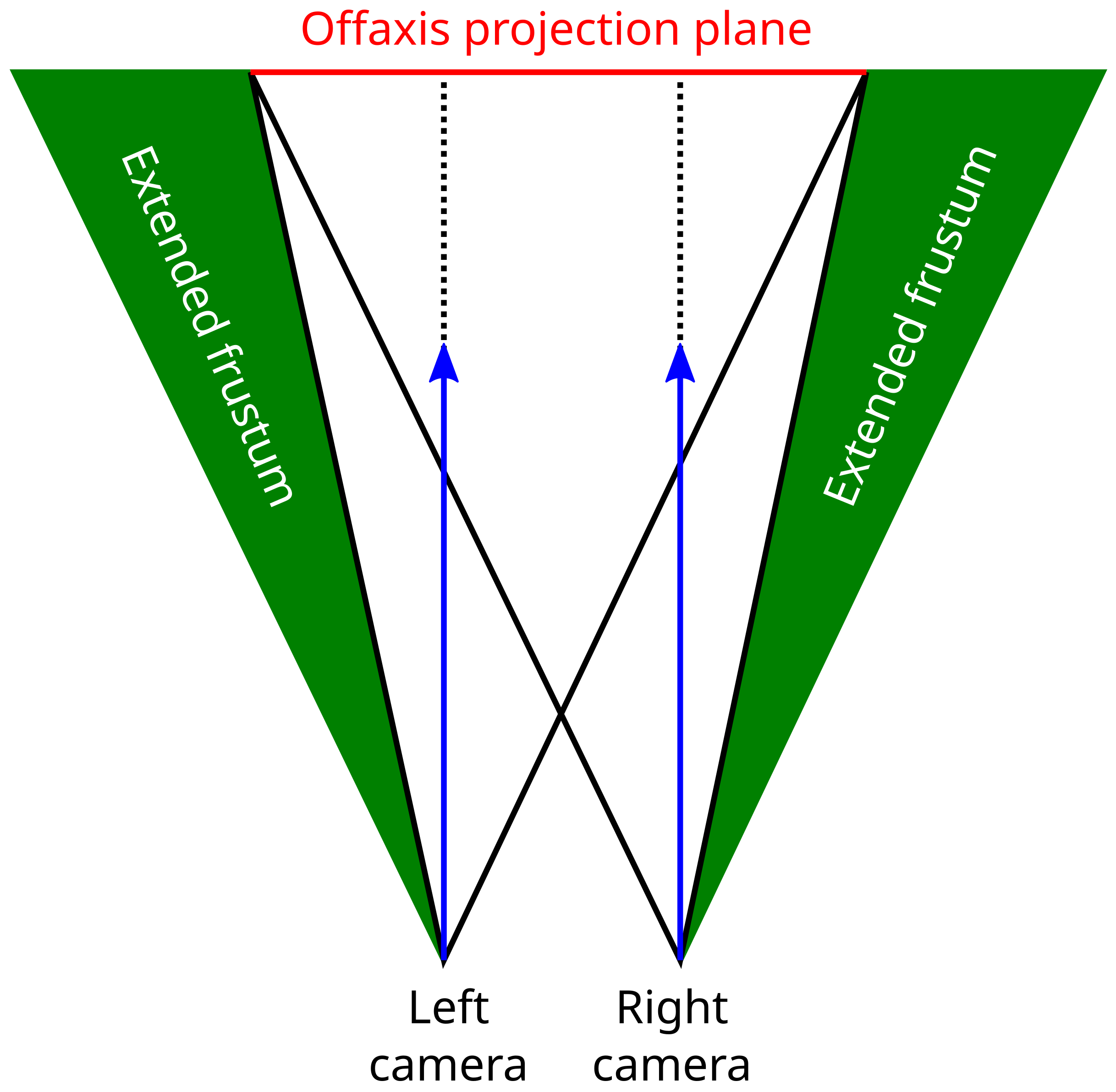
2.2. Stereo Rendering

One special feature of our renderer is the support for rendering stereo images. There are multiple approaches to setting up stereo rendering, but not all yield accurate results. The correct approach for stereo projection is the off-axis method, as it prevents the introduction of vertical parallax. Vertical parallax occurs when the eyes are misaligned vertically, leading to visual discomfort and an inaccurate stereo effect. This can be prevented by aligning the central viewing directions of both cameras in parallel, while each camera focuses on a different point (see Figure 3). This ensures a natural and comfortable stereo effect. Thus, it is necessary to render two images with different camera view frustums. However, the two extended camera frustums do not overlap completely. To obtain the off-axis projection plane of both images, one has to trim the projection of the extended frustums. Therefore, one has to compute the non-overlapping amount of pixels $\delta$ [36]:

$$\delta ={\displaystyle \frac{b·w}{2·f_o·tan\left(\frac{\alpha }{2}\right)}},$$

(7)

where w is the image width in pixels and $f_o$ is the focal length. b is the stereo base, i.e., half of the camera x-offset. The angle of view $\alpha$ can be computed as follows:

$$\begin{array}{cc}\hfill \alpha & =2·arctan\left({\displaystyle \frac{d}{2·f_o}}\right)\hfill \\ \hfill & =2·arctan\left({\displaystyle \frac{1}{f_o}}\right),\hfill \end{array}$$

(8)

where d is the width of the normalized image plane. In our case, $d=2$ because the range of the normalized image plane goes from −1 to 1. Now, if a stereo image of resolution $w\times$ h is rendered, first, this resolution will be extended by $\delta$. Then, the left and right images with a resolution of $(w+\delta )\times$ h are rendered. Finally, to obtain the off-axis projection plane, both images are trimmed to $w\times h$ again.

3. Materials and Methods

3.1. Performance Realization

3.1.1. GPU Architecture and CUDA Implementation

To leverage modern hardware capabilities, we employed the NVIDIA CUDA toolkit, which provides an interface for highly parallelized computation on GPUs. Since CUDA is only available for NVIDIA devices, we were restricted in the choice of the graphic card. Moreover, the renderer was developed using MATLAB^® 2023a while relying on CUDA 10.2, which needs compatible devices.

CUDA provides a special CUDA-C compiler. This GPU device code can easily be connected to the host (CPU) C++ code. The host code provides some data structures and functions that handle the communication between the host and device. Using the MATLAB^® mex interface, we built a MATLAB^® command. For this purpose, MATLAB^® provides a special compiler that translates all the compiled C object files into a MATLAB^® command. As the MATLAB^® renderer command requires a lot of parameters, we developed some wrapper classes with special properties to make the handling more comfortable. Compilation is straightforward and performed inside MATLAB^® using make.m, mex, and mexcuda. Users only need to set up a compatible compiler and install CUDA by following the provided instructions.

3.1.2. Ray Casting on GPU

Ray casting involves shooting rays from the viewer or camera through the volume to determine the accumulated light intensity as the rays traverse it. Each ray is tested for an intersection with the volume only once per rendering pass, as we support rendering one object per pass. We implemented a simplified version of the fast intersection test introduced by [37], which is effective for scenarios involving a single intersection per ray and avoids complex data structures.

The world coordinate frame is centered within the volume, with a scalar d representing the distance from the volume. The camera is positioned along the negative z-axis, with the projection plane set at a distance of 1 from the camera, as illustrated in Figure 4. The focal length $f_o$ can be adjusted, and the camera can be rotated around the object using a rotation matrix R.

The projection plane is defined in normalized coordinates ranging from $[-1, -1]$ to $[1, 1]$. Each pixel value on the rendered image is determined by projecting the corresponding x and y coordinates of the ray onto the normalized projection plane coordinates u and v. With all this information, we can compute the direction of a ray and its origin with

$$\begin{array}{cc}\hfill di{r}_{ray}& ={\displaystyle \frac{u·\overrightarrow{x}+v·\overrightarrow{y}+f_o·\overrightarrow{z}}{\left|\right|u·\overrightarrow{x}+v·\overrightarrow{y}+f_o·\overrightarrow{z}\left|\right|}}\hfill \\ \hfill ori{g}_{ray}& =c_o·\overrightarrow{x}+(-1)·d·\overrightarrow{z}\hfill \end{array}$$

(9)

where $\overrightarrow{x}$, $\overrightarrow{y}$, and $\overrightarrow{z}$ are the particular column vectors of the rotation matrix, and $c_o=\pm b$ represents half of the total x-offset between the two cameras, which can be defined by the user.

By utilizing the GPU for computation, each ray—representing one pixel of the rendered image—is processed by a separate CUDA thread. This approach achieves a high level of parallelization, resulting in an efficient and fast rendering program that would be challenging to parallelize and compute effectively on a CPU alone.

3.1.3. Memory Management

GPU memory is very limited and not extendable. Usually, our renderer requires six different volumes: one for emission, one for absorption, one for reflection, and one for each gradient direction. If all these volumes are copied to the GPU, this might lead to a high memory consumption. In some cases, these volumes can be similar or they differ only by a scalar factor, e.g., one can have an emission volume $vo{l}_{em}$ and an absorption volume $vo{l}_{ab}=k_{ab}·vo{l}_{em}$. Due to the texture mapping NVIDIA CUDA provides to perform efficient lookups, it is possible to map one volume to multiple textures [38]. This enabled us to map $vo{l}_{em}$ to $te{x}_{ab}$. To provide the possibility that the looked-up value is multiplied by a scalar factor, the renderer is enabled to set up one scalar multiplicator for the emission, absorption, and reflection volumes. To be able to save more GPU memory, one can set up the renderer to compute the gradient on the fly. As expected this is computationally more expensive, especially if a movie sequence of one scene is rendered. Figure 5 shows the possible options.

The illumination volume and the light sources are copied to the GPU memory as well. Volumes are only copied to the device if they have been modified since the last rendering process. This minimizes the host-to-GPU transactions and increases the rendering performance of scenes with multiple images. All the texture lookups use trilinear interpolation.

3.1.4. Illumination Model and LUT Optimization

In order to provide some degree of freedom for the illumination model, we employed a 3D lookup table. The lookup table describes the interaction of a particle with a light source, as depicted in Figure 6. Since we know where the light source and the view point are located, the unit vector of the incoming light ${\overrightarrow{L}}_i$ and the unit vector of the outgoing light ${\overrightarrow{L}}_o$ are known. ${\overrightarrow{L}}_o$ equals the view direction. The normal vector $\overrightarrow{n}$ is approximated by the negative gradient and then normalized. As described in Section 3.1.3, the gradient is either determined by $vo{l}_{\nabla }$ or computed on the fly using the finite difference scheme. With this information, the angles $\alpha$ and $\beta$ can be computed.

$\gamma$ is the angle between ${\overrightarrow{L}}_i^{\prime }$ and ${\overrightarrow{L}}_o^{\prime }$, the projections of ${\overrightarrow{L}}_i$ and ${\overrightarrow{L}}_o$ onto the surface plane. We can compute these vectors using vector projection as follows:

$$\begin{array}{c}\hfill {\overrightarrow{L}}_i^{\prime }={\overrightarrow{L}}_i-\langle {\overrightarrow{L}}_i,\overrightarrow{n}\rangle \overrightarrow{n},\\ \hfill {\overrightarrow{L}}_o^{\prime }={\overrightarrow{L}}_o-\langle {\overrightarrow{L}}_o,\overrightarrow{n}\rangle \overrightarrow{n},\end{array}$$

(10)

where $\langle \overrightarrow{a},\overrightarrow{b}\rangle$ denotes the dot product between the two vectors $\overrightarrow{a}$ and $\overrightarrow{b}$. After the calculation of these angles, the light intensity can be established by performing a lookup. Since the LUT contains only a finite number of entries, trilinear interpolation is applied. The underlying LUT can be built up with a lot of isotropic illumination models.

Henyey–Greenstein

Our renderer uses the Henyey–Greenstein phase function to compute the light intensity (see Equation (5)). The corresponding LUT is built up with the angles $\alpha$, $\beta$, and $\gamma$. Unfortunately, $\theta$ is the angle between ${\overrightarrow{L}}_i$ and ${\overrightarrow{L}}_o$. Thus, we had to compute $\theta$ for each $\alpha$, $\beta$, and $\gamma$. In order to compute the LUT we chose

$${\overrightarrow{L}}_o=\left(\begin{array}{c}sin\left(\alpha \right)\\ 0\\ cos\left(\alpha \right)\end{array}\right), {\overrightarrow{L}}_i=\left(\begin{array}{c}sin\left(\beta \right)\\ 0\\ cos\left(\beta \right)\end{array}\right)$$

(11)

while $\alpha$ and $\beta$ are iterated dependent on the resolution of the LUT. To perform the rotation around the surface normal, we built a rotation matrix ${\mathbf{R}}_{\overrightarrow{n}}$ around the surface normal dependent on $\gamma$. Aligning with the properties of the unit circle, we applied the rotation around the x-axis. ${\overrightarrow{L}}_i$ is kept fixed while ${\overrightarrow{L}}_o$ is rotated. Now, $\theta$ is computed by using the dot product:

$$\begin{array}{c}\hfill \overrightarrow{rot}={\mathbf{R}}_{\overrightarrow{n}}{\overrightarrow{L}}_o,\\ \hfill \theta =arccos(\langle \overrightarrow{rot},{\overrightarrow{L}}_i\rangle ).\end{array}$$

(12)

The angles $\alpha$, $\beta$, and $\gamma$ are all constrained to the range $[0, \pi ]$ due to the inherent symmetries of the light and view interactions with the surface normal. $\alpha$ and $\beta$ describe the angles between the surface normal and the light or view directions. Due to the symmetry of the surface, the orientation of the light or view direction on either side of the normal produces equivalent angles. Similarly, $\gamma$, which represents the relative rotation of the projected light and view vectors within the surface plane, also exhibits symmetry, as angles beyond $\pi$ are redundant and equivalent to their complementary angles within $[0, \pi ]$. By restricting the angles to this range, we maintained consistency and efficiency in the representation and computation of the illumination model. The angles are expressed in radians and allow for the LUT creation using Equation (5) as follows:

$$\begin{array}{c}\hfill \mathrm{LUT}(a,b,c)=HG(\theta ,g).\end{array}$$

(13)

where $\alpha =a·{\displaystyle \frac{\pi }{n}}$, $\beta =b·{\displaystyle \frac{\pi }{n}}$, and $\gamma =c·{\displaystyle \frac{\pi }{n}}$. n denotes the resolution of the LUT. Because the three angles are iterated, we end up in a three-time nested loop. To obtain a high performance, we decided to implement the computation of the LUT in C++ and provide API bindings to MATLAB^®. Thus, we provided a fast computation of this LUT via a MATLAB^® command. The parameters are the resolution of the LUT and g (see Equation (5)). As mentioned before, the LUT contains only a finite number of entries. Thus, during a lookup, a trilinear interpolation is applied. Furthermore, CUDA requires lookup values to be normalized within the range of 0 to 1. The process of looking up lighting is illustrated in Algorithm 1.

Algorithm 1 Pseudo-code for the ‘shade’ function of our renderer. This function calculates the illumination at a given voxel position by evaluating the contributions of multiple light sources, considering the surface normal, view direction, and reflection properties. The algorithm iteratively processes each light source using texture lookups for reflection and illumination to determine the light contribution to the voxel’s appearance.

Require: $aSamplePosition$, $aPosition$, $aGradientStep$, $aViewPosition$

Require: $aColor$, $aLightSources$, $aFactorReflection$, $aSurfaceNormal$

Ensure: Calculated light contribution at the given voxel position

1:  $result\leftarrow \mathbf{0}$

2:  for each $lightSource$ in $aLightSources$ do

3:   $lightPosition\leftarrow lightSource.position$

4:   $lightOut\leftarrow \mathrm{normalize}(lightPosition-aPosition)$

5:   $lightIn\leftarrow \mathrm{normalize}(aViewPosition-aPosition)$

6:   $\overrightarrow{n}\leftarrow \mathrm{normalize}\left(aSurfaceNormal\right)$

7:   $\alpha \leftarrow \mathrm{angle}(\overrightarrow{n}, lightOut)$

8:   $\beta \leftarrow \mathrm{angle}(\overrightarrow{n}, lightIn)$

9:   $lightOutProj\leftarrow \mathrm{normalize}(lightOut-(\mathrm{dot}(lightOut, \overrightarrow{n})·\overrightarrow{n}))$

10:   $lightInProj\leftarrow \mathrm{normalize}(lightIn-(\mathrm{dot}(lightIn, \overrightarrow{n})·\overrightarrow{n}))$

11:   $\gamma \leftarrow \mathrm{angle}(lightInProj, lightOutProj)$

12:   $reflection\leftarrow aFactorReflection·\mathrm{lookupTextureReflection}\left(aSamplePosition\right)$

13:   $light\leftarrow \mathrm{lookupTextureIllumination}({\displaystyle \frac{\alpha }{\pi }},{\displaystyle \frac{\beta }{\pi }},{\displaystyle \frac{\gamma }{\pi }})$

14:   $result\leftarrow result+(reflection·light·lightSource.color·aColor)$

15:  end for

16:  return  $result$

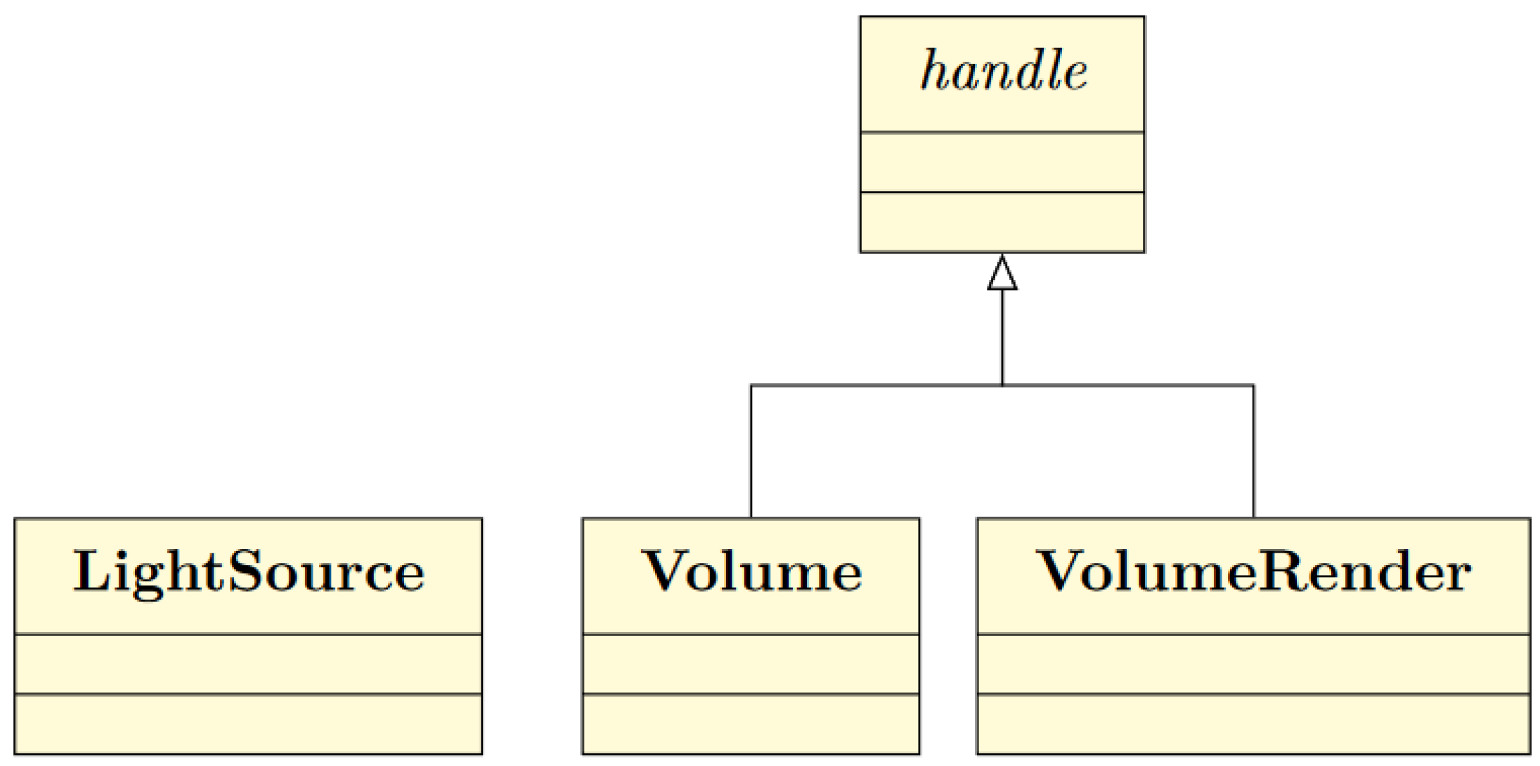
3.2. MATLAB^® Interface

The compiled MATLAB^® command of the volume renderer requires several input parameters. Thus, we decided to write complementary wrapper classes to further simplify the developer experience (see Figure 7).

Handle Superclass

The realization of the memory management described in Section 3.1.3 requires special techniques on the part of MATLAB^®. Usually a MATLAB^® class member works with call by value. But since we require the possibility to check the pointer of the volumes, call by reference is necessary. More precisely, on the C++ side, we want to check whether the volumes are pointing to different pointer addresses or to the same one. Consequently, only the unique volume data are copied to the GPU, whereas the other assignments are realized by texture mapping to the assigned volume data. For us, this seemed to be the most user-friendly way to implement our memory model.

Usually, a regular value assignment via a setter can be costly because it replaces the old object with a new one, which is then returned. Fortunately, MATLAB^® offers the possibility for call by reference. A class that inherits from the special handle superclass automatically uses call by reference instead of call by value [39]. Hence, the class Volume inherits handle. Through this, all properties stored in a Volume object are pointers.

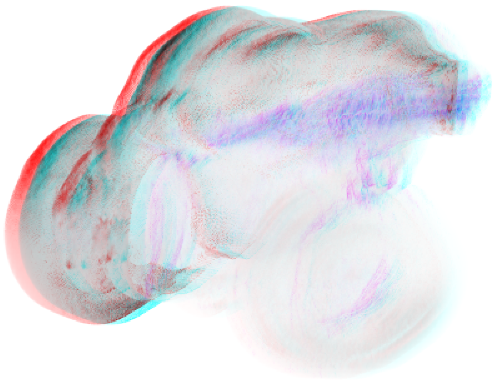
3.3. Case Study

3.3.1. Dataset

To demonstrate the capabilities of the renderer, we used a volumetric dataset of a zebrafish larva (ViBE-Z_72hpf_v1) created with ViBE-Z [40]. Zebrafish embryos are widely used as a model organism in developmental biology and neurobiology due to their transparency and rapid development. High-resolution volumetric data of zebrafish larvae were acquired using 3D microscopy, providing detailed images of the internal structures essential for various research purposes. ViBE-Z uses multiple confocal microscope stacks and a fluorescent stain of cell nuclei for image registration and enhances the data quality through fusion and attenuation correction. ViBE-Z can detect 14 predefined anatomical landmarks for aligning new data to the reference brain and can perform a colocalization analysis in expression databases for anatomical domains or subdomains. Specifically, the dataset used in this work contains zebrafish larval datasets. These include average silhouettes and brain structures with multiple channels. Each channel corresponds to different fluorescent markers that highlight various anatomical features. Specifically, we used data representing the average brain anatomy and the expression patterns of the 3A10-marked neural structure in the zebrafish embryo, with a volume resolution of 800 × 500 × 500 voxels. These volumetric data are stored in an HDF5 file.

In addition to the zebrafish dataset, we utilized the Brain Tumor Segmentation 2020 (BraTS2020) dataset [41,42,43], which is a collection of multi-modal human MRI scans used for the development and evaluation of brain tumor segmentation algorithms. It includes preoperative MRI scans with three modalities: T1-weighted, T1-weighted with contrast, and T2-weighted, all with associated ground truth segmentations. The dataset is annotated with tumor regions, including enhancing tumors, core tumors, and whole tumors, providing a comprehensive resource for training and benchmarking segmentation models. The images in BraTS2020 have a resolution of 240 × 240 × 155 voxels and are stored in the NIfTI format.

3.3.2. Scene

In our rendering scenario, we created a movie depicting a 3D scene. The illumination setup was configured with a single light source that emitted white light positioned at [−15, 15, 0]. The LUT, configured with a resolution of 64 × 64 × 64, utilized the Henyey–Greenstein phase function with an asymmetry parameter of $g=0.8$. Parameters such as the element size, focal length (set to 3.0 scene units), distance to the object (6 scene units), rotation angles, and an opacity threshold (0.95) were defined to put the object into the scene. For the zebrafish embryo, the scene unit corresponded to micrometers (µm), which reflected the fine-scale resolution of the dataset. In contrast, for the BraTS2020 brain dataset, the scene unit was in millimeters (mm), consistent with the typical scale of medical imaging datasets. The image resolution was configured based on the dimensions of the volume data. The emission and absorption volumes were set to the same data. The reflection volume was set to 1 for each voxel. The gradient was computed on the fly by the GPU.

In the rendering process, the zebrafish average brain image underwent a multi-step transformation. Initially, the entire volume was rendered with emission and absorption factors set to 1, which resulted in a fully illuminated scene. Subsequently, a fading effect to the interior and half or the entire embryo was applied, which gradually reduced its visibility until we eventually ended up with the shell of one-half of the average brain structure. This effect was achieved by adjusting the emission intensity of the volume data with the help of a pre-computed mask.

The rendering of the 3A10-marked neural structure did not experience any manipulations but was rendered using an emission factor of 0.5 and an absorption factor of 1. After each rendering, the scene was rotated to provide a dynamic view from different angles. The rotation angles were calculated to achieve a rotation of 1200° over the course of the movie. The entire rendering consisted of three rendering loops:

• Rotation of the average brain by 150° (30 image frames);
• Fading out of the interior and one-half while rotating 900° (180 image frames);
• Rotation of half of the average brain shell by 150° (30 image frames);
• Rendering of the 3A10-marked neural structure with full rotation of 1200° (240 image frames).

Finally, the rendered frames from the average brain channel and the structure channel were combined to create a composite visualization of the zebrafish embryo. The resulting 240-image movie provided a complete visualization of the volumetric data that revealed structural details and expression patterns within the embryo. In this process, to enhance the visualization, a square root normalization was applied to the combined volumes, which amplified the visibility after inversion during the post-processing. The final inverted images provided higher print quality and improved contrast. Stereo rendering was optionally enabled to generate anaglyph images for three-dimensional viewing, achieved by offsetting the camera along the x-axis.

Analogous to the previously described approach, we utilized the BraTS2020 dataset. Instead of using an average brain model, we employed the T1 scan of an individual human brain. Additionally, instead of the 3A10-marked structure, the annotated ground truth tumor data from the particular brain scan were used.

The scenes were rendered on a mobile workstation running Win11 with an NVIDIA A5000 with 16 GB VRAM and an Intel Core i9 11950H with 2.6 GHz, 64 GB RAM, and an SSD.

4. Results

4.1. Implementation

Our memory manager was designed to be user-friendly, offering MATLAB^® classes that streamline the process of memory management. This allows users to easily allocate, deallocate, and manage memory within their MATLAB^® projects without delving into complex CUDA programming. The source code is openly available on GitHub, making it accessible to the research and development community. This openness fosters innovation and allows for continuous improvement based on collective expertise and user feedback.

4.2. Volume Design

Our renderer supports the capability to define each volume, i.e., emission, absorption, and reflection, allowing for custom renderings to simulate different materials with different light properties. This is possible to do at a fine granular scale for each voxel by defining distinct volumes or for an entire volume by a scalar. For our zebrafish volume, Figure 8 shows the stepwise variations in the scale values $k_{em}$, $k_{ab}$, and $k_{ref}$. The rendering setup was similar to the scene, but the absorption volume was set to a volume with value 1 for each voxel. The visual impact of the scales and, therefore, the different volumes became clearly discernible.

Without any emission, absorption, and reflection information, the image was not visible. On the other hand, while increasing the absorption and adding some reflection, the opacity increased, as the light was reflected and absorbed by the object. High reflection values led to a shiny appearance, which could be counteracted by absorption, while no reflection at all made the object disappear. Increasing the emission signals increased the effects. Although this illustration demonstrated the effect on the entire volume using the scaling values, it is important to emphasize that it is certainly possible to manipulate an object’s voxels to achieve specific effects in targeted areas. Boolean operations with masking can be used to select areas of interest.

4.3. Case Study

The rendered images effectively captured the fine details of the zebrafish embryo anatomy. By adjusting the emission, absorption, and reflection parameters, the visualizations effectively differentiated between various tissue types and fluorescent markers. The illumination setup further enhanced the depth and contrast of the images, which made the internal structures more discernible. Our case study consisted of 240 rendered images that contained the zebrafish embryo average brain and the 3A10-marked neural structure. The fish was rotated by 1200° and one-half of the average brain faded out in that image sequence. Figure 9 shows an excerpt of eight images in which the object was rotated 360°. The GPU rendering took 119.32 s for the 240 images on our hardware setup.

Specifically, the first sequence, which corresponded to the 150° rotation of the average brain, took 4.57 s; the second, which involved the 900° rotation with fading out of the interior and one-half of the brain, took 58.58 s; and the third, which rotated half of the brain shell by 150°, took 6.22 s. The rendering of the 3A10-marked neural structure with a full 1200° rotation took 49.95 s. The second scene was the most computationally expensive due to the fading effect that required data synchronization with the GPU for each frame, which led to a runtime of 0.33 s per frame, while the other scenes averaged 0.20 s per frame, which reflected the costs of host-to-GPU data transfers. The computation of the LUT only took 0.55 s. This time was not included in the numbers mentioned before. The GPU memory load was around 2 GiB.

For the second dataset, our case study involved processing a single MRI volume from the BraTS2020 dataset. Figure 10 shows an excerpt from the rendered scene demonstrating the tumor regions. The rendering on our hardware setup took 9.69 s for the 240 images. Specifically, the first sequence, which corresponded to the 150° rotation of the T1-weighted brain scan, took 0.40 s. The second sequence, which involved the 900° rotation and the fading of the brain’s interior and one-half, took 5.32 s. The third sequence, which rotated half of the brain shell by 150°, took 0.47 s. The final sequence, which rendered the tumor region with a full 1200° rotation, took 3.50 s. The segmentation and fading operations were the most computationally intensive, which contributed to the variation in the processing times across the different scenes. The average memory load during processing was around 1.2 GiB.

Finally, the ability to generate stereo images and animations add another layer of depth to the visualizations, making it easier to comprehend the spatial relationships between different anatomical features. These realistic visualizations not only aid in detailed anatomical studies but also serve as valuable tools for educational purposes, providing clear and comprehensible images of complex biological structures. Figure 11 shows an image of the zebrafish scene rendered in stereo using anaglyph. All three described renderings can be seen in full length in the Supplementary Materials.

5. Discussion

5.1. Principal Findings

Our work offers a feature-rich offline renderer designed to support a wide range of functionalities. To keep the complexity limited, we employed a simplified volume-rendering equation, allowing for a highly parallelized GPU-based implementation. Since the GPU memory size is very limited, the memory management we designed provides the opportunity to render volumes of larger resolutions. Moreover, the rendering equation works with absorption and emission. Thus, it is possible to set up the rendering configuration to render multiple volumes in separated rendering passes in a way that the combination forms a composite visualization.

Our illumination model interface enables the use of different illumination equations than those proposed in this work. Several light sources with various light color intensities can be defined. This increases the realism of the scene, and thus, the spatial impression of the scene.

The MATLAB^® interface was optimized for simplified usage so that one can easily construct visualizations, such as movie scenes and static images. Moreover, our renderer can render stereo images and combine them into an anaglyph or Side-By-Side stereo image. Since the values of the rendered images are stored as float types, the interface also provides normalization methods for both single-image and whole-image sequences. Finally, we optimized the runtime of the MATLAB^® code. In order to be able to realize the memory management, we made use of the handle class of MATLAB^®, which allowed us to use call by reference instead of call by value. In conclusion, we provide a new convenient MATLAB^® tool for volume rendering.

MATLAB^®’s built-in Medical Image Labeler, introduced in R2022b, complemented our work by providing interactive 3D visualization with direct volume rendering, alongside annotation and segmentation tools. It supports both 2D images and 3D image volume data in DICOM, NIfTI, and NRRD formats, seamlessly integrating with MATLAB^®’s broader ecosystem. While the Medical Image Labeler excels in its user-friendly interface and annotation capabilities, our system focuses on delivering a high degree of control over the rendering parameters, offering advanced lighting and material configurations that go beyond the built-in features. This combination of tools within MATLAB^® offers researchers a robust suite for image analysis and detailed volumetric rendering, enabling them to potentially derive insights from their data [6].

5.2. Limitations

Modern deep learning approaches support features such as up-scaling [44], allowing for end-to-end training from image examples and eliminating the need for manual feature design while supporting advanced visualization concepts, like shading and semantic colorization [45], or even real-time rendering [46]. In contrast, our renderer lacks these advanced features out of the box but offers flexibility, enabling fully adjustable emission, absorption, and reflection parameters, along with customizable illumination setups. Also, our approach does not require extensive and potentially expensive training of models. However, one challenge might be the complexity of the configuration options, which could overwhelm some users and might require training.

An important aspect to note is that in our shading approach, the gradient is normalized, which results in a loss of information about its original magnitude. However, it is possible to use the gradient magnitude to determine the strength of surface reflection, which can influence how reflectivity is defined based on the surface properties. Our flexible model is capable of incorporating such an adjustment. Specifically, the gradient magnitude could be computed as a separate volume within the preprocessing phase, for instance, in MATLAB^®, and then referenced within the reflection volume during rendering. This would allow for the integration of gradient magnitude information directly into the surface reflection computation.

Furthermore, although volume operations are a valuable feature, any modifications to the volume require a costly transfer back to the GPU. For example, masking in our scene had to be performed outside the GPU. As a result, the rendering times are heavily affected by the scene complexity. Therefore, the provided timings are meant to give a general impression rather than precise benchmarks.

Additionally, while MATLAB^®’s Medical Image Labeler provides robust tools for 3D visualization and annotation, it does not offer the same level of control over rendering as our system. Users looking for highly customizable lighting and material properties may find our tool more suited to their needs. However, the complexity and potential learning curve associated with our tool’s configuration options could be a limitation for users seeking a more straightforward solution.

Lastly, the renderer’s integration with MATLAB^®, while powerful, may limit its usability for those unfamiliar with MATLAB^® or those working in environments where other software is preferred.

5.3. Future Work

To increase the realism and spatial impression of the rendered scenes, the renderer could be enabled to use some shadowing techniques, as described in [47], or more sophisticated shading techniques, as described in [48]. Furthermore, our renderer uses trilinear interpolation. To obtain more accurately interpolated values, tri-cubic interpolation could be added as an additional option.

Furthermore, to increase the usability and simplify the setup, the renderer could be extended with a user interface. An additional view showing the positioning of the light sources would also be beneficial. This could then also be extended for the development of video sequences in order to easily create camera paths and object motions by means of interpolation. However, these points are not planned to be implemented by us for the time being, but could be addressed by the community.

6. Conclusions

We demonstrated the effectiveness of our GPU-enabled renderer in visualizing zebrafish embryo volumetric data with high realism. The flexibility in adjusting the rendering parameters and the ability to create detailed, immersive visualizations make this tool an excellent choice for both research and educational applications. This integration with MATLAB^® provides a robust platform for biomedical researchers to analyze and visualize complex volumetric datasets within a familiar environment.

References

- Kaufman, A.E. 43—Volume Visualization in Medicine. In Handbook of Medical Imaging; Bankman, I.N., Ed.; Biomedical Engineering; Academic Press: San Diego, CA, USA, 2000; pp. 713–730. [Google Scholar] [CrossRef]
- de Oliveira Santos, B.F.; da Costa, M.D.S.; Centeno, R.S.; Cavalheiro, S.; de Paiva Neto, M.A.; Lawton, M.T.; Chaddad-Neto, F. Clinical Application of an Open-Source 3D Volume Rendering Software to Neurosurgical Approaches. World Neurosurg. 2018, 110, e864–e872. [Google Scholar] [CrossRef] [PubMed]
- Smit, N.; Bruckner, S. Towards Advanced Interactive Visualization for Virtual Atlases. In Biomedical Visualisation: Volume 3; Rea, P.M., Ed.; Springer International Publishing: Cham, Switzerland, 2019; pp. 85–96. [Google Scholar] [CrossRef]
- Hernandez-Cortés, K.S.; Mesa-Pujals, A.A.; García-Gómez, O.; Montoya-Arquímedes, P. Brain morphometry in adult: Volumetric visualization as a tool in image processing. Rev. Mex. Neurocienc. 2021, 22. [Google Scholar] [CrossRef]
- Huang, S.H.; Irawati, N.; Chien, Y.F.; Lin, J.Y.; Tsai, Y.H.; Wang, P.Y.; Chu, L.A.; Li, M.L.; Chiang, A.S.; Tsia, K.K.; et al. Optical volumetric brain imaging: Speed, depth, and resolution enhancement. J. Phys. Appl. Phys. 2021, 54, 323002. [Google Scholar] [CrossRef]
- Zhou, L.; Fan, M.; Hansen, C.; Johnson, C.R.; Weiskopf, D. A Review of Three-Dimensional Medical Image Visualization. Health Data Sci. 2022, 2022, 9840519. [Google Scholar] [CrossRef]
- Dickie, D.A.; Shenkin, S.D.; Anblagan, D.; Lee, J.; Blesa Cabez, M.; Rodriguez, D.; Boardman, J.P.; Waldman, A.; Job, D.E.; Wardlaw, J.M. Whole Brain Magnetic Resonance Image Atlases: A Systematic Review of Existing Atlases and Caveats for Use in Population Imaging. Front. Neuroinform. 2017, 11, 1. [Google Scholar] [CrossRef]
- Diao, B.; Bagayogo, N.A.; Carreras, N.P.; Halle, M.; Ruiz-Alzola, J.; Ungi, T.; Fichtinger, G.; Kikinis, R. The use of 3D digital anatomy model improves the communication with patients presenting with prostate disease: The first experience in Senegal. PLoS ONE 2022, 17, e0277397. [Google Scholar] [CrossRef]
- Kikinis, R.; Pieper, S.D.; Vosburgh, K.G. 3D Slicer: A Platform for Subject-Specific Image Analysis, Visualization, and Clinical Support. In Intraoperative Imaging and Image-Guided Therapy; Jolesz, F.A., Ed.; Springer: New York, NY, USA, 2014; pp. 277–289. [Google Scholar] [CrossRef]
- Schindelin, J.; Arganda-Carreras, I.; Frise, E.; Kaynig, V.; Longair, M.; Pietzsch, T.; Preibisch, S.; Rueden, C.; Saalfeld, S.; Schmid, B.; et al. Fiji: An open-source platform for biological-image analysis. Nat. Methods 2012, 9, 676–682. [Google Scholar] [CrossRef] [PubMed]
- Royer, L.A.; Weigert, M.; Günther, U.; Maghelli, N.; Jug, F.; Sbalzarini, I.F.; Myers, E.W. ClearVolume: Open-source live 3D visualization for light-sheet microscopy. Nat. Methods 2015, 12, 480–481. [Google Scholar] [CrossRef]
- Jarrett, T.; Comrie, A.; Sivitilli, A.; Pretorius, P.C.; Vitello, F.; Marchetti, L. iDaVIE: Immersive Data Visualisation Interactive Explorer. 2024. Available online: https://zenodo.org/records/13752029 (accessed on 18 June 2024).
- Selvamanikkam, M.; Noga, M.; Khoo, N.S.; Punithakumar, K. High-Resolution Stereoscopic Visualization of Pediatric Echocardiography Data on Microsoft HoloLens 2. IEEE Access 2024, 12, 9776–9783. [Google Scholar] [CrossRef]
- Fujii, Y.; Azumi, T.; Nishio, N.; Kato, S.; Edahiro, M. Data Transfer Matters for GPU Computing. In Proceedings of the 2013 International Conference on Parallel and Distributed Systems, Seoul, Republic of Korea, 15–18 December 2013; pp. 275–282. [Google Scholar] [CrossRef]
- Gao, H.; Liu, Y.; Cao, F.; Wu, H.; Xu, F.; Zhong, S. VIDAR: Data Quality Improvement for Monocular 3D Reconstruction through In-situ Visual Interaction. In Proceedings of the 2024 IEEE International Conference on Robotics and Automation (ICRA), Yokohama, Japan, 13–17 May 2024; pp. 7895–7901. [Google Scholar] [CrossRef]
- Hu, J.; Fan, Q.; Hu, S.; Lyu, S.; Wu, X.; Wang, X. UMedNeRF: Uncertainty-Aware Single View Volumetric Rendering For Medical Neural Radiance Fields. In Proceedings of the 2024 IEEE International Symposium on Biomedical Imaging (ISBI), Athens, Greece, 27–30 May 2024; pp. 1–4, ISSN 1945-8452. [Google Scholar] [CrossRef]
- Dhawan, A.P. Medical Image Analysis; John Wiley & Sons: Hoboken, NJ, USA, 2011. [Google Scholar]
- Reyes-Aldasoro, C.C. Biomedical Image Analysis Recipes in MATLAB: For Life Scientists and Engineers; John Wiley & Sons: Hoboken, NJ, USA, 2015. [Google Scholar]
- Mathotaarachchi, S.; Wang, S.; Shin, M.; Pascoal, T.A.; Benedet, A.L.; Kang, M.S.; Beaudry, T.; Fonov, V.S.; Gauthier, S.; Labbe, A.; et al. VoxelStats: A MATLAB Package for Multi-Modal Voxel-Wise Brain Image Analysis. Front. Neuroinform. 2016, 10, 20. [Google Scholar] [CrossRef]
- Wait, E.; Winter, M.; Cohen, A.R. Hydra image processor: 5-D GPU image analysis library with MATLAB and python wrappers. Bioinformatics 2019, 35, 5393–5395. [Google Scholar] [CrossRef] [PubMed]
- Interactively Explore, Label, and Publish Animations of 2-D or 3-D Medical Image Data-MATLAB-MathWorks Deutschland. Available online: https://de.mathworks.com/help/medical-imaging/ref/medicalimagelabeler-app.html (accessed on 14 September 2024).
- Explore 3-D Volumetric Data with Volume Viewer App-MATLAB & Simulink-MathWorks Deutschland. Available online: https://de.mathworks.com/help/images/explore-3-d-volumetric-data-with-volume-viewer-app.html (accessed on 30 August 2022).
- Kroon, D.J. Volume Render. Available online: https://de.mathworks.com/matlabcentral/fileexchange/19155-volume-render (accessed on 30 August 2022).
- Robertson, S. Ray Tracing Volume Renderer. Available online: https://de.mathworks.com/matlabcentral/fileexchange/37381-ray-tracing-volume-renderer (accessed on 30 August 2022).
- Röttger, S.; Kraus, M.; Ertl, T. Hardware-Accelerated Volume and Isosurface Rendering Based on Cell-Projection; ACM, Inc.: New York, NY, USA, 2000. [Google Scholar]
- Wiki, O. Vertex Rendering—OpenGL Wiki. 2022. Available online: https://www.khronos.org/opengl/wiki/vertex_Rendering (accessed on 23 May 2024).
- Lorensen, W.E.; Cline, H.E. Marching cubes: A high resolution 3D surface construction algorithm. SIGGRAPH Comput. Graph. 1987, 21, 163–169. [Google Scholar] [CrossRef]
- Levoy, M. Display of Surfaces from Volume Data. IEEE Comput. Graph. Appl. 1988, 8, 29–37. [Google Scholar] [CrossRef]
- Max, N.L. Optical Models for Direct Volume Rendering. IEEE Trans. Vis. Comput. Graph. 1995, 1, 99–108. [Google Scholar] [CrossRef]
- Wikipedia. Volume Ray Casting—Wikipedia, The Free Encyclopedia. 2023. Available online: http://en.wikipedia.org/w/index.php?title=Volume%20ray%20casting&oldid=1146671341 (accessed on 18 April 2023).
- Shannon, C.E. Communication in the presence of noise. Proc. Inst. Radio Eng. IRE 1949, 37, 10–21. [Google Scholar] [CrossRef]
- Henyey, L.; Greenstein, J. Diffuse radiation in the galaxy. Astrophys. J. 1941, 93, 70–83. [Google Scholar] [CrossRef]
- Porter, T.; Duff, T. Compositing digital images. In Proceedings of the 11th Annual Conference on Computer Graphics and Interactive Techniques, SIGGRAPH ’84, New York, NY, USA, 23–27 July 1984; pp. 253–259. [Google Scholar] [CrossRef]
- Bavoil, L.; Myers, K. Order independent transparency with dual depth peeling. NVIDIA OpenGL SDK 2008, 1, 2–4. [Google Scholar]
- Ikits, M.; Kniss, J.; Lefohn, A.; Hansen, C. Rendering. In GPU GEMS Chapter 39, Volume Rendering Techniques, 5th ed.; Addison Wesley: Boston, MA, USA, 2007; Chapter 39.4.3. [Google Scholar]
- Bourke, P. Calculating Stereo Pairs. 1999. Available online: http://paulbourke.net/stereographics/stereorender (accessed on 8 September 2022).
- Williams, A.; Barrus, S.; Morley, R.K.; Shirley, P. An Efficient and Robust Ray-Box Intersection Algorithm. J. Graph. Gpu Game Tools 2005, 10, 49–54. [Google Scholar] [CrossRef]
- NVIDIA Corporation. NVIDIA CUDA C Programming Guide. Version 8.0. 2017. Available online: https://docs.nvidia.com/cuda/archive/8.0/pdf/CUDA_C_Programming_Guide.pdf (accessed on 8 September 2022).
- The MathWorks, I. Comparison of Handle and Value Classes-MATLAB & Simulink -MathWorks Deutschland. Available online: https://de.mathworks.com/help/matlab/matlab_oop/comparing-handle-and-value-classes.html (accessed on 18 September 2024).
- Ronneberger, O.; Liu, K.; Rath, M.; Rueß, D.; Mueller, T.; Skibbe, H.; Drayer, B.; Schmidt, T.; Filippi, A.; Nitschke, R.; et al. ViBE-Z: A framework for 3D virtual colocalization analysis in zebrafish larval brains. Nat. Methods 2012, 9, 735–742. [Google Scholar] [CrossRef]
- Menze, B.H.; Jakab, A.; Bauer, S.; Kalpathy-Cramer, J.; Farahani, K.; Kirby, J.; Burren, Y.; Porz, N.; Slotboom, J.; Wiest, R.; et al. The Multimodal Brain Tumor Image Segmentation Benchmark (BRATS). IEEE Trans. Med. Imaging 2015, 34, 1993–2024. [Google Scholar] [CrossRef]
- Bakas, S.; Akbari, H.; Sotiras, A.; Bilello, M.; Rozycki, M.; Kirby, J.S.; Freymann, J.B.; Farahani, K.; Davatzikos, C. Advancing The Cancer Genome Atlas glioma MRI collections with expert segmentation labels and radiomic features. Sci. Data 2017, 4, 170117. [Google Scholar] [CrossRef] [PubMed]
- Bakas, S.; Reyes, M.; Jakab, A.; Bauer, S.; Rempfler, M.; Crimi, A.; Shinohara, R.T.; Berger, C.; Ha, S.M.; Rozycki, M.; et al. Identifying the Best Machine Learning Algorithms for Brain Tumor Segmentation, Progression Assessment, and Overall Survival Prediction in the BRATS Challenge. arXiv 2019, arXiv:1811.02629. [Google Scholar]
- Devkota, S.; Pattanaik, S. Deep Learning based Super-Resolution for Medical Volume Visualization with Direct Volume Rendering. arXiv 2022, arXiv:2210.08080. [Google Scholar]
- Weiss, J.; Navab, N. Deep Direct Volume Rendering: Learning Visual Feature Mappings From Exemplary Images. arXiv 2021, arXiv:2106.05429. [Google Scholar]
- Hu, J.; Yu, C.; Liu, H.; Yan, L.; Wu, Y.; Jin, X. Deep Real-time Volumetric Rendering Using Multi-feature Fusion. In Proceedings of the ACM SIGGRAPH 2023 Conference, SIGGRAPH ’23, New York, NY, USA, 6–10 August 2023; pp. 1–10. [Google Scholar] [CrossRef]
- Ikits, M.; Kniss, J.; Lefohn, A.; Hansen, C. Volumetric Lighting. In GPU GEMS Chapter 39, Volume Rendering Techniques, 5th ed.; Addison Wesley: Boston, MA, USA, 2007; Chapter 39.5.1. [Google Scholar]
- Ament, M.; Dachsbacher, C. Anisotropic Ambient Volume Shading. IEEE Trans. Vis. Comput. Graph. 2016, 22, 1015–1024. [Google Scholar] [CrossRef]
Disclaimer/Publisher’s Note: The statements, opinions and data contained in all publications are solely those of the individual author(s) and contributor(s) and not of MDPI and/or the editor(s). MDPI and/or the editor(s) disclaim responsibility for any injury to people or property resulting from any ideas, methods, instructions or products referred to in the content. |
© 2024 by the author. Licensee MDPI, Basel, Switzerland. This article is an open access article distributed under the terms and conditions of the Creative Commons Attribution (CC BY) license (https://creativecommons.org/licenses/by/4.0/).
Share and Cite
Scheible, R. GPU-Enabled Volume Renderer for Use with MATLAB. Digital 2024, 4, 990-1007. https://doi.org/10.3390/digital4040049
Scheible R. GPU-Enabled Volume Renderer for Use with MATLAB. Digital. 2024; 4(4):990-1007. https://doi.org/10.3390/digital4040049
Chicago/Turabian StyleScheible, Raphael. 2024. "GPU-Enabled Volume Renderer for Use with MATLAB" Digital 4, no. 4: 990-1007. https://doi.org/10.3390/digital4040049
APA StyleScheible, R. (2024). GPU-Enabled Volume Renderer for Use with MATLAB. Digital, 4(4), 990-1007. https://doi.org/10.3390/digital4040049