Design of Open Code Software to Downs and Steiner Lateral Cephalometric Analysis with Tracing Landmarks

Abstract

Cephalometric analysis is an excellent instrument in clinical diagnosis, treatment, and recovery from surgery. Nowadays, efforts to develop computerized dental X-ray image Cephalometric analysis systems for clinical and education usages. Much commercial software is created, but its high cost is unaffordable for some undergraduate students or low-income medical institutions; sure, the best option is the use of open source software alternatives. The study aimed to design free software Cephalopoint that applies vector algebra to perform the accuracy and precision of Cephalometric analysis. Three tests were used to validate the measurements made: accuracy test, consisting of comparing three selected cases and reply 32 times using the manual and software technique measurement; time test, consisted in obtaining the average time used to complete manual and software techniques of the previous test; and statistical test, consisted of measuring and applying the statistical analysis of 42 random cases for each method only using the software technique. The results showed high repeatability and no significant difference between manual tracing and software techniques. All the variables calculated with the software technique exhibited a normal distribution. Cephalopoint is excellent software for accurate and precise Cephalometric measurements. Moreover, it significantly decreased the measurement time compared with the manual.

1. Introduction

The Cephalometric is a set of tracing planes generated by some combination of Cephalometric points in lateral cranial radiography; the measurement of the length between Cephalometric points and the angle formed by Cephalometric planes gives a descriptive and predictive tool of patient craniofacial development [1]. The Cephalometric is a principal diagnostic method because it allows us to study skeletal, dental, and soft tissue aspects, dental-maxillary anomalies, dental misalignment, and malocclusion of dentoskeletal origin [2]. Furthermore, it evaluates orthodontic treatment progress and surgical outcomes of dentofacial deformity treatment [3].

Typically, Cephalometric analysis has been performed manually by tracing landmarks on patient radiography and measuring linear and angular variables. The technique is time-consuming and has several drawbacks by the dentists, including errors during hand tracing, landmark identification, and measurement [4,5,6]. The software is not only used to assist measurement; it could be applied to aid the carrying out and planning of orthodontic treatment or orthognathic surgery, such as TFA [7].

Around the world, many universities offer dental clinical services to local communities where undergraduate students practice. Typically, the patients have to attend one day to take the X-ray radiography and return another day to hear the diagnostics; this could be made more efficient if the dentists would reduce the time expended in measuring and analyzing the Cephalometry. The software application has demonstrated very usefully to minimize the time inverted.

There are several commercial alternatives to perform the technique; among them, we can mention Quick Ceph, Dolphin, Nemoceph, Vistadent, TraceCeph, CephX, and Facad. Using the software is very helpful for orthodontic practitioners in performing Cephalometric analysis and determining diagnostic and treatment plans. However, the cost of the purchase of this software is quite expensive [8].

Some health institutions have the income to obtain a limit of commercial software licenses, and not all undergraduate dentists have access to computers with one of these licenses. In developing countries with low and medium-income would be challenging to buy a license.

Medical services are inaccessible for almost 100 million people who live in extreme poverty [9]. Many governments and civil association campaign programs exist to carry these services to marginal communities. The accuracy and time expended are crucial factors in these campaigns.

The engineering faculty continually finds ways to give back to society with our science and technology knowledge. Software measuring the Cephalometric angles and distances based on vector algebra was designed. The software is offered as freeware and allows other programmers to use it as open source.

Cephalopoint is an open source software code programmed on Octave; each code applied vector and matrix operations to measure the Cephalometric traces according to Downs and Steiner’s Analysis. Octave was selected as the platform to develop the software because it has a set of commands to convert images, do matrix and vector operations, and plot tools in many ways. Furthermore, it offers the possibility to incorporate routines from other programmers to upgrade the code helping to do image processing to recognize the Cephalometric points or use special statistical libraries.

Measurements were made comparing the precision, repeatability, and time invested by the manual technique and software provided. Cephalopoint application showed accuracy in the results very close to manually; the time expended was a third part of the manual technique.

The measurements obtained by software technique were analyzed statistical variables. The values analyzed showed normal distribution and correct behavior.

2. Materials and Methods

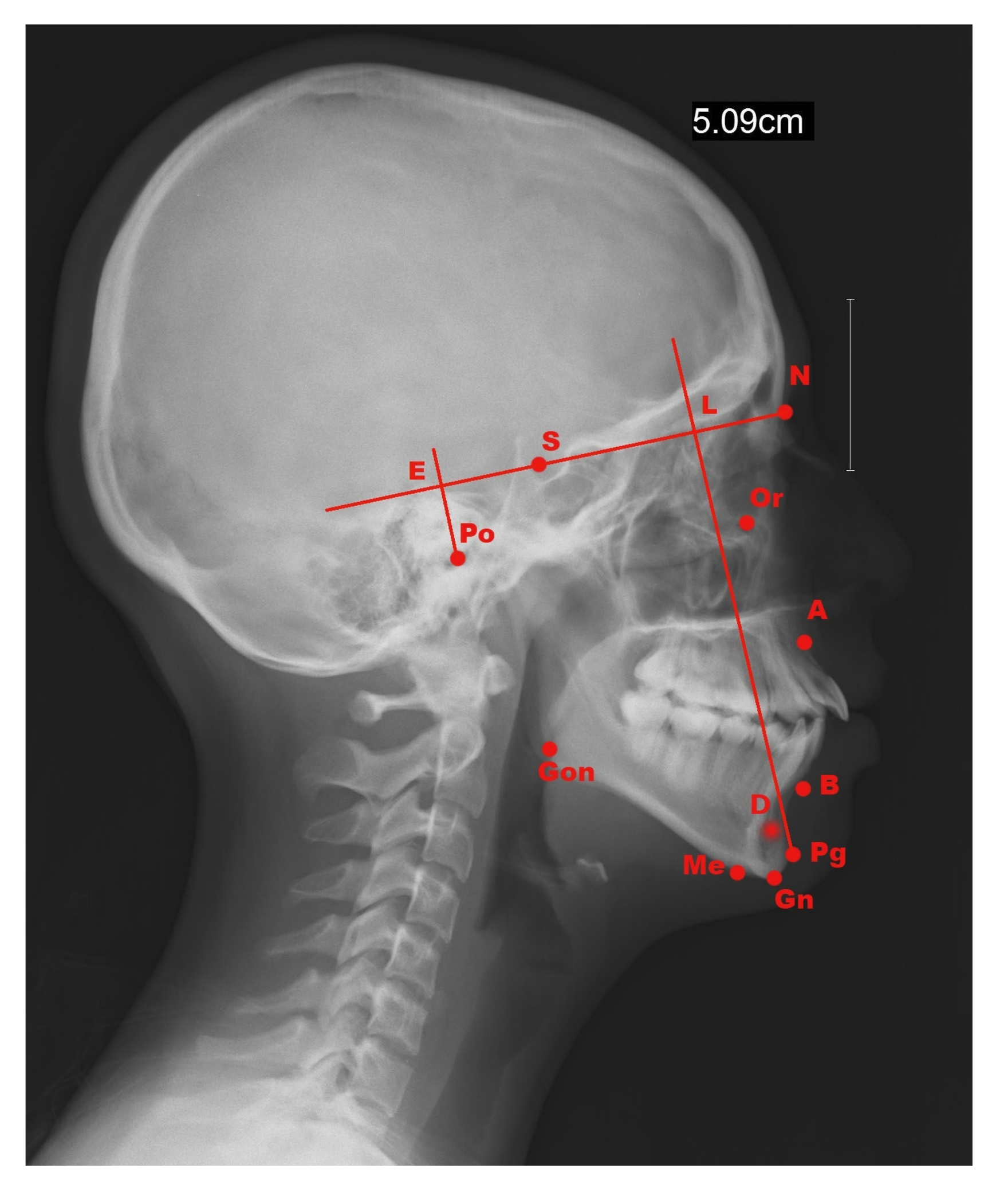
2.1. Cephalometric Methods

The Lateral Cephalometric analysis is based on the correct position of the landmarks, as seen in Figure 1.

The principal difference between Downs’ and Steiner’s Cephalometric is the use of different Cephalometric planes and angles.

Downs Cephalometric Analysis is the measurement to identify skeletal malformations by relating the various Cephalometric points and planes [10,11]. Tracking the planes and angles formed by Cephalometric points is necessary to determine the skeletal malformations, as shown in

Table 1. Downs’ Lateral Cephalometric measurements and norms.

Measurement	Landmarks	Standard Value
Facial Angle	PoOr-NPg	$82\pm 2°$
Convexity Angle	NA-APg	$0\pm 1°$
AB Plane Angle	AB-NPg	$-4.6\pm 2°$
Mandibular Plane Angle	PoOr-GoMe	$21.9\pm 3°$
Y Angle	SGn-PoOr	$59.4\pm 4°$
Occlusal Angle	PoOr-O.P.	$9.5\pm 2°$
Interincisal Angle	I.A.	$135.4\pm 4°$
Lower incisor to O.P.	L.I.-O.P.	$14.5\pm 2°$
Lower incisor to Mandibular Plane	L.I.-GoMe	$90\pm 4°$
Upper incisor to APg	U.I.-APg	$2.7\pm 4$ mm

. Downs’ analysis is typically used in children and adolescents who are still growing.

Steiner Cephalometric Analysis is the measurement of craniofacial structures based on the analysis by tracing and locating lateral facial landmarks; Frankfort plane (PoOr) is not used in this analysis [1,11]. The anatomic points formed the planes and angles to obtain the clinical data, as shown in

Table 2. Steiner’s Lateral Cephalometric measurements and norms.

Measurement	Landmarks	Standard Value
SNA	SN-NA	$82\pm 2°$
SNB	SN-NB	$80\pm 3°$
SND	SN-ND	$76\pm 2°$
ANB	AN-NB	$2\pm 2°$
NSG	NS-SGn	$65\pm 3°$
SNGoGn	SN-GoGn	$32\pm 4°$
SL Segment	S-L	$51\pm 4$ mm
SE Segment	S-E	$22\pm 3$ mm
O.P. to SN	O.P.-SN	$14\pm 3°$
Interincisal Angle	I.A.	$131\pm 4°$
Upper incisor to NA	U.I.-NA	$22\pm 6°$
Upper incisor to SN	U.I.-SN	$103\pm 4°$
Lower incisor to NB	L.I.-NB	$25\pm 4°$

. Steiner’s analysis is typically used in adults whose growth is already finished.

2.2. Software Designed

The software was designed as an Octave’s Library, formed by four files: Two file codes to create the headers of Downs’ and Steiner’s landmarks of reservoir corresponding files. One file code to do Downs’ analysis and another Steiner’s analysis. The library is available to download from the Cephalopoint website [12].

A graphical interface was necessary created to make the software friendlier. The version of Octave used was 6.2.0; it does not have an interface to create applications or bottoms like Matlab. Still, it is possible to emulate a graphic interface using a modal dialog box containing one or more text edit fields and returns the values entered by the user.

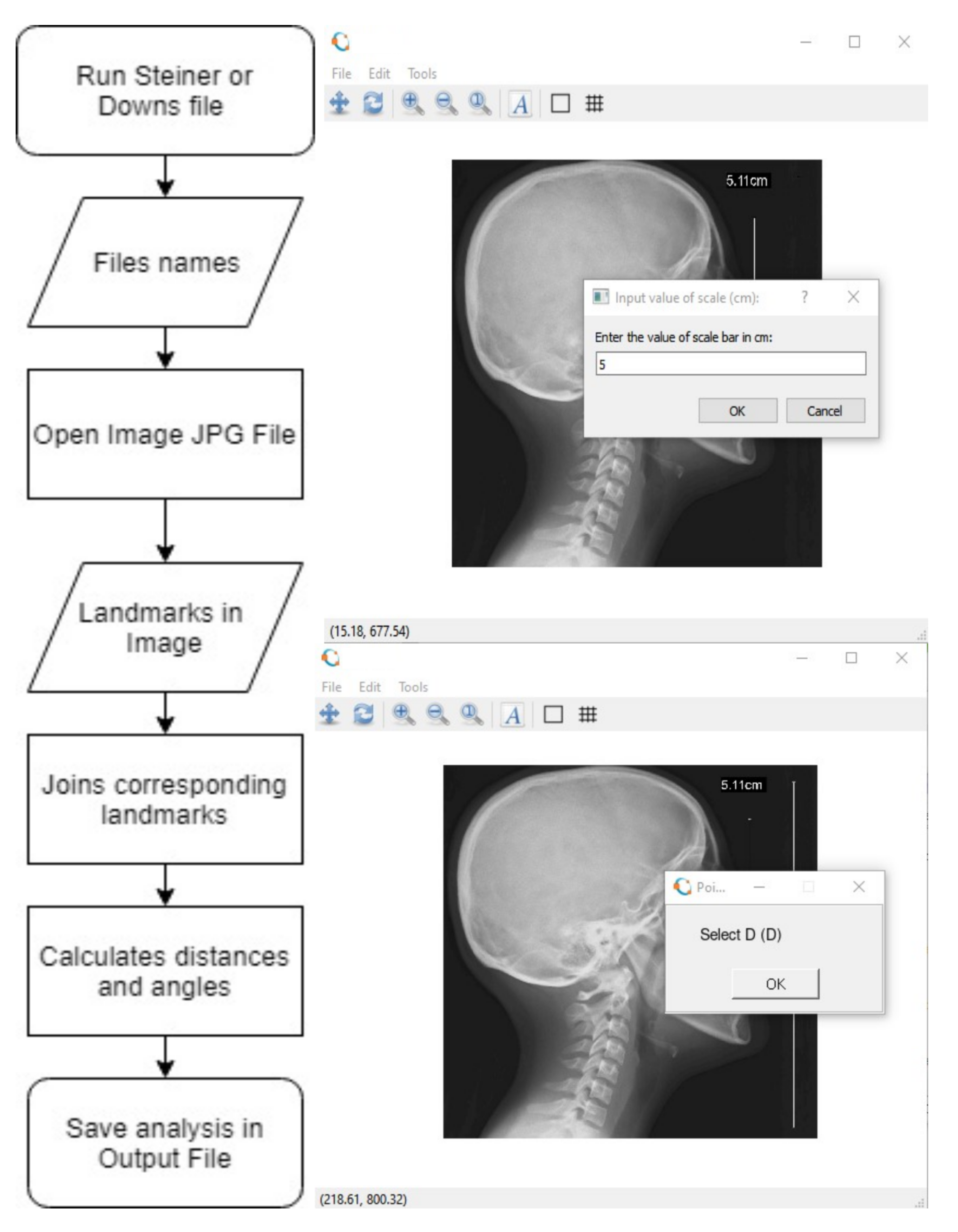
The logic used to program Cephalopoint is described by the following flowchart diagram, as shown in Figure 2. Initially, select one of the Cephalometric techniques routine. The software opens a dialog box where the name of the JPG Cephalometric file, an output file to save the results, and the size of the scale bar would be written. Then the code opens the image selected and will ask for the landmark points. The code will calculate the size of the vectors and the angles between planes, applying the concepts shown in Appendix A; finally, the measures will be saved at the output file previously selected.

The measurements would be saved to a comma-separated value (CSV) output file. It is helpful for dentists to perform statistical, clinical analysis, as it could be used in any spreadsheet.

2.3. Accuracy and Time Tests

Sample: Three different cases for each method were studied 32 times using manual and software techniques.

Manual Technique Materials: The research materials used were digital Cephalograms in JPEG format and printed. Research tools used were tracing paper, negatoscope, 4H pencil, adhesive (taped), protractor (Baum), rule, erasers, Hardware: Laptop HP ProBook Core i5 2.30 GHz, Memory RAM 4 GB, Intel HD Graphics Family; software Windows 7 and Octave. The object of this study was the digital X-rays obtained from Orthopantomograph OP300 of the patients. Downs and Steiner lateral Cephalometric analysis using conventional techniques was performed by tracing landmarks on tracing paper of the printed Cephalogram. On each sample Cephalogram, the determination of Downs’ and Steiner’s reference points (as seen in Figure 1), lines and planes drawing, angle and distance measurement using protractor and rule were conducted.

Software Technique: The same cases and times were analyzed using Cephalopoint and saved in the respective output file.

Time Measure: The Manual and Software techniques were chronometric each time and compared the average obtained in each method.

Accuracy Measure: The mean (m) and standard error ($S_e$) of each Downs’ and Steiner’s variables were calculated and compared for each case.

$$S_e=\frac{S}{\sqrt{n}}$$

(1)

where n is the number of samples and S is the standard deviation.

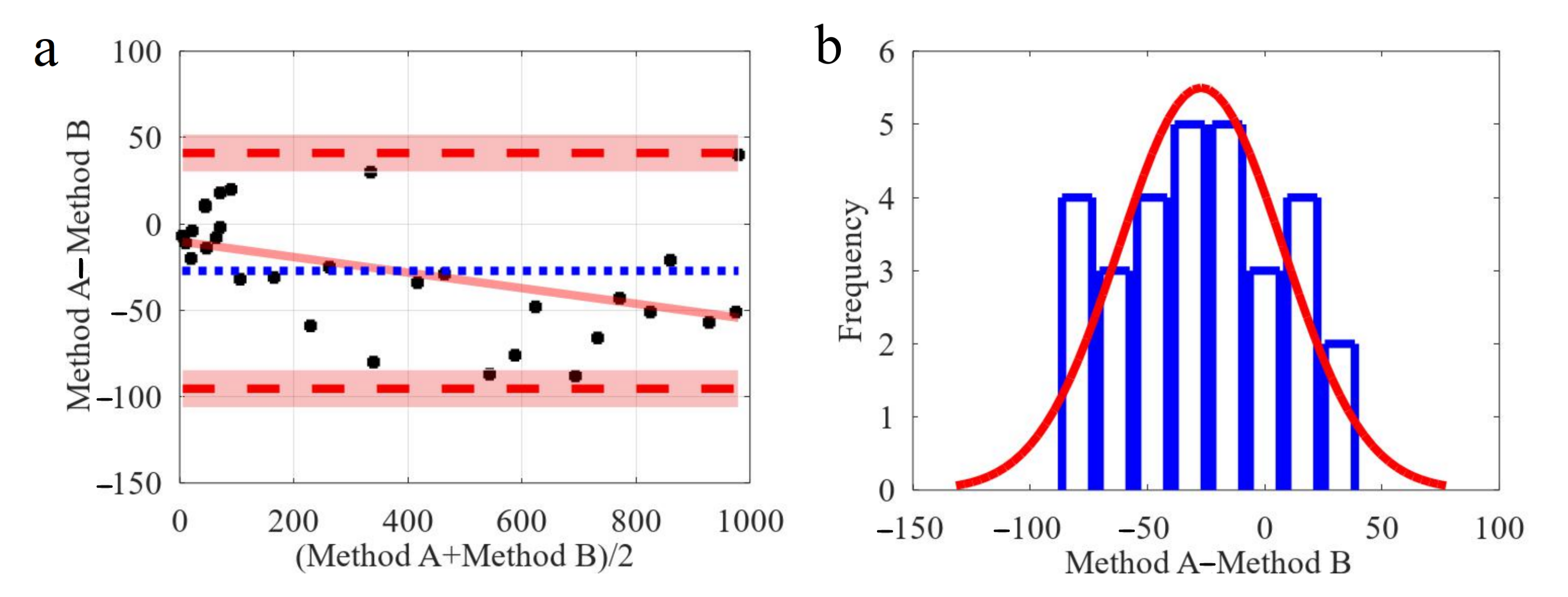
Bland–Altman Analysis: It was proposed as an alternative analysis based on quantifying the agreement between two quantitative measurements by studying the mean difference and constructing limits of agreement. The Bland–Altman plot analysis is a simple way to evaluate a bias between the mean differences and estimate an agreement interval, within which 95% of the differences of the second method, compared to the first one, fall [13]. The graph displays a scatter diagram of the differences plotted against the averages of the two measurements. Horizontal lines are drawn at the mean difference and the limits of agreement, as seen in Figure 3a. The regression line of the difference could help in detecting a proportional difference [14]. The plot allows to evaluate the global agreement between two measurements.

Normal distribution of the differences must always be verified by drawing a histogram, as seen in Figure 3b. The statistical test should always be used to determine if the distribution is normal since, in some cases, normality cannot be determined simply by observing the histogram plot. A test for normal distribution (such as the Shapiro–Wilk test) can be done for the hypothesis that the distribution of the observations in the sample is normal (if p < 0.05, then reject normality). If differences are not normally distributed, a logarithmic transformation of original data can be tried [13].

Intra and inter-operator reproducibility were compared and analyzed using Bland–Altman analysis.

Repeatability Coefficient: The repeatability coefficient ($RC$) is a precision measure that represents the value below which the absolute difference between two repeated test results may be expected to lie with a probability of 95% [15].

$$RC=1.96\sqrt{2}S$$

(2)

2.4. Statistical Test

Patient Demographics: The study sample contains 84 patients (32 M, 52 F) treated in the Orthodontics Clinic of the university from Mar 2017 until July 2017. Two formed groups: Steiner’s analysis group selected 42 patients (20 M, 22 F); mean age $54\pm 12$; ranging from 20 to 72 years. Downs’ analysis group set 42 patients (18 M, 24 F); mean age $13\pm 5$; ranging from 7 to 19 years.

Sample Size Calculation: The sample size calculation had on Downs’ and Steiner’s norms variables and their standard deviation values. The significance level ranged at 5% and a confidence level of 95%. Thus, a sample of 36 patients in each group would give 88% power under these circumstances. In consequence, 42 patients were established as the sample size for both groups.

Kurtosis: (K) is a statistical measure that is used to describe the distribution. Kurtosis measures extreme values in either tail. Distributions with large kurtosis exhibit tail data exceeding the tails of the normal distribution. Distributions with low kurtosis exhibit tail data that are generally less extreme than the tails of the normal distribution [16].

$$K=\frac{\mathrm{Mean}({(x_i-m)}^4)}{S^4}$$

(3)

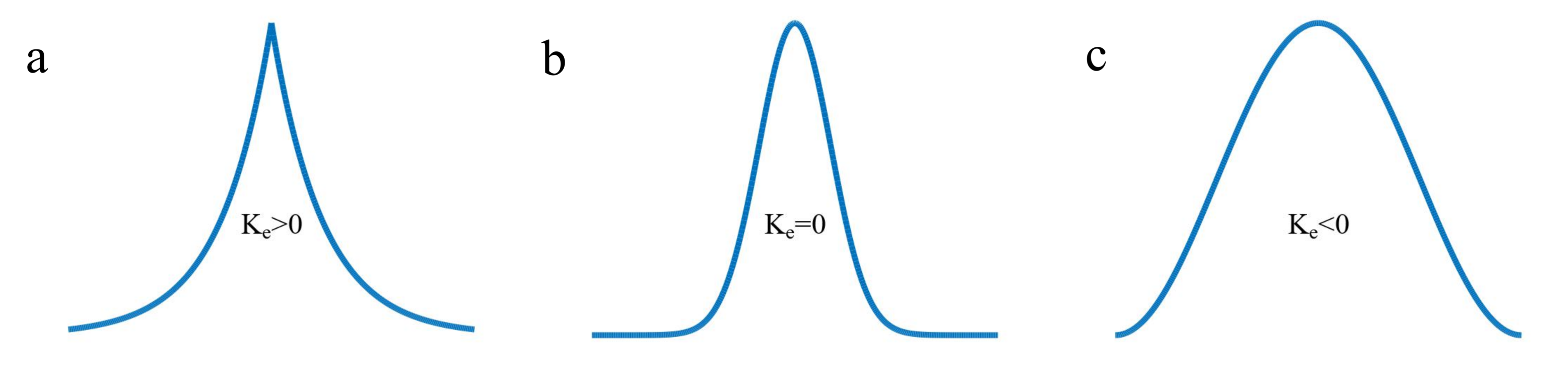
The excess kurtosis ($K_e$) is defined as kurtosis minus 3. There are three distinct regimes as described below.

$$K_e=K-3$$

(4)

There are three categories of kurtosis that a set of data can display. All measures of kurtosis are compared against a standard normal distribution [17].

Leptokurtic distribution $K_e>0$. Leptokurtic has very long and skinny tails, which means there are more chances of outliers. Positive values of kurtosis indicate that distribution is peaked and possesses thick tails. An extreme positive kurtosis indicates a distribution where more numbers are located in the distribution’s tails instead of around the mean (Figure 4a).

Mesokurtic distribution $K_e\approx 0$. Mesokurtic is the same as the normal distribution, which means kurtosis is near to 0. In Mesokurtic, distributions are moderate in breadth, and curves are a medium peaked height (Figure 4b).

Platykurtic distribution $K_e<0$. Platykurtic having a lower tail and stretched around center tails means most data points are in high proximity with mean. A platykurtic distribution is a flatter (less peaked) when compared with the normal distribution (Figure 4c).

To establish a criterion of decision between which values of $K_e$ could be considered as a mesokurtic distribution, the adjusted Fisher-Pearson standardized moment coefficient of skewness ($G_1$) was considered.

$$G_1=\frac{n}{(n-1)(n-2)}\mathrm{Sum}{\left(\frac{x_i-m}{S}\right)}^3$$

(5)

The lower and upper limits were established as 90% range for sample skewness coefficient $G_1$ [18].

The Shapiro–Wilk test (W) is a way to tell if a random sample comes from a normal distribution. The test gives a W value; small values indicate the sample is not normally distributed (you can reject the null hypothesis that the population is normally distributed if your values are under a certain threshold) [19]. The domain of W is restricted to the interval (0,1).

$$W=\frac{{(\mathrm{Sum}(a_i{x}_{(i)}))}^2}{\mathrm{Sum}{(x_i-m)}^2}$$

(6)

where, $x_{(i)}$ (with parentheses enclosing the subscript index i; not to be confused with $x_i$) is the ith order statistic; $a_i$ are constants generated from the covariances, variances, and means of the sample (size n) from a normally distributed sample.

The coefficients $a_i$ are given by:

$$(a_1,\dots ,a_n)=\frac{m^T{V}^{-1}}{C}$$

(7)

where C is a vector norm:

$$C=\sqrt{u^T{V}^{-1}{V}^{-1}u}$$

(8)

Furthermore, the vector u,

$$u={(u_1,\dots ,u_n)}^T$$

(9)

It is made of the expected values of the order statistics of independent and identically distributed random variables sampled from the standard normal distribution; finally, V is the covariance matrix of those normal order statistics [20].

Since you use tables the W will be between two values: $W_1$ and $W_2$, and the p-value (p) between the relevant two p-values: $p_1$ and $p_2$. Calculate the approximate p-value using a linear ratio.

$$p=p_1+\frac{W-W_1}{W_2-W_1}(p_2-p_1)$$

(10)

The null hypothesis of this test is that the population is normally distributed. Thus, if the $p<0.05$, then the null hypothesis is rejected and there is evidence that the data tested are not normally distributed. On the other hand, if the $p>0.05$, then the null hypothesis (that the data came from a normally distributed population) can not be rejected.

The data was analyzed using an Octave’s code programmed by Nir Krakauer [21] based on the study of Patrick Royston [22]. This code was validated comparing the value of $W=0.8797$ calculated with $W=0.8812$ observed on the study of Shapiro and Wilk [23]. Other data tables were analyzed, and the correspondence between these values is excellent.

3. Results

The results of the Cephalometric Manual and Software techniques were analyzed according to the tests proposed. The results are shown according to each test.

3.1. Time Test

Table 3. Downs’ and Steiner’s Lateral Cephalometric average time for 3 different cases.

Technique	Downs’ Cephalometric			Steiner’s Cephalometric
	Case 1	Case 2	Case 3	Case 1	Case 2	Case 3
Manual	18.5 min	17.3 min	16.7 min	17.1 min	16.4 min	18.2 min
Software	5.6 min	6.3 min	6.4 min	5.2 min	5.8 min	6.5 min

shows the average time used by each case and method after 32 times.

The average time to realize all manual techniques was 17.4 min per patient compared with the average time to realize all software techniques was 6 min per patient.

3.2. Accuracy Test and Techniques Comparison

3.2.1. Downs’ Cephalometric

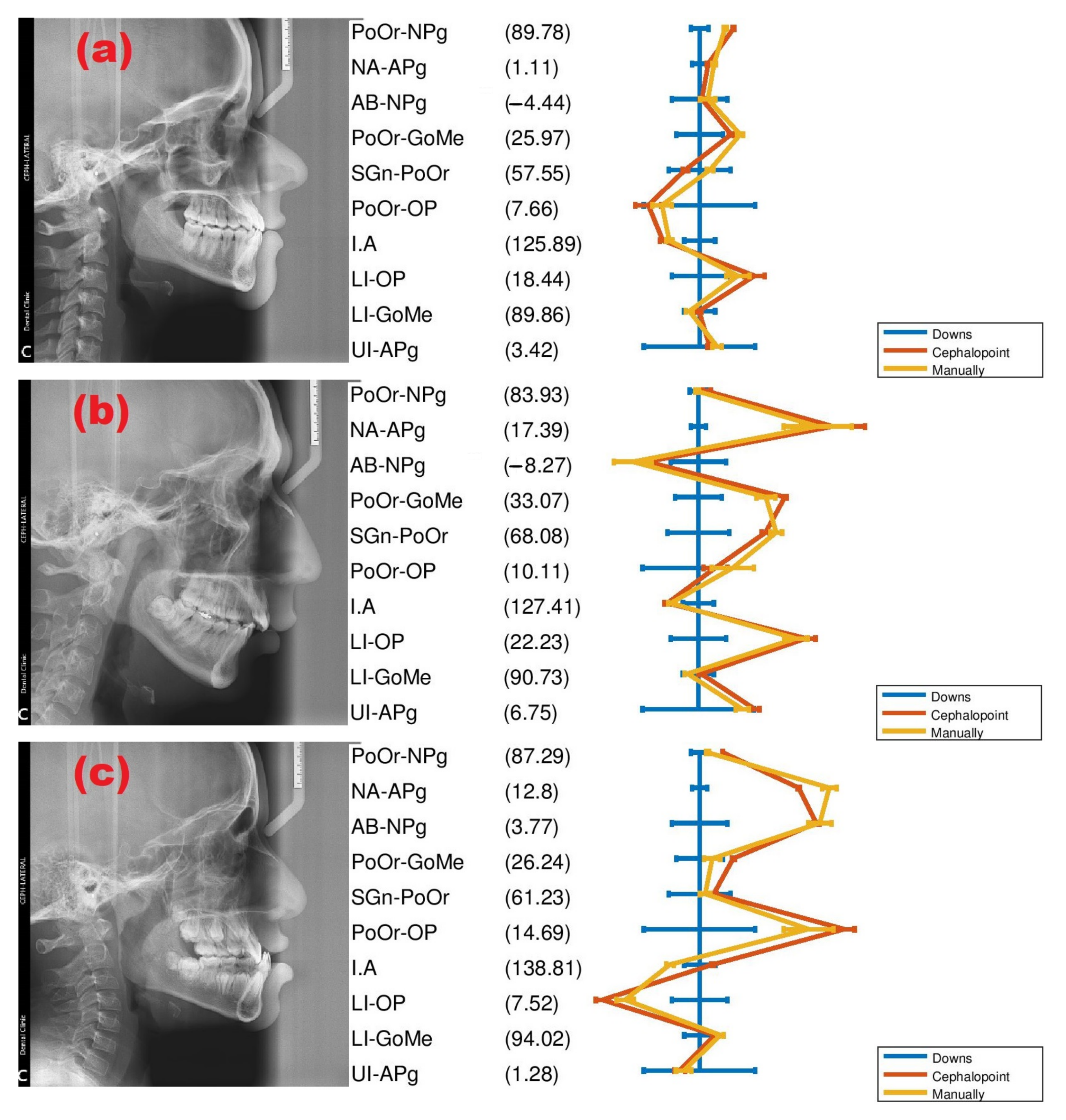
Case 1 (Figure 5a) was classified as skeletal class I, normal chin with suggestive increased lower incisor proclination. Case 2 (Figure 5b) was classified as skeletal class II, suggesting a prominent maxillary denture base with the mandible and unfavorable face, also indicates vertical growth pattern of the mandible, and suggestive of increased lower incisor proclination. Moreover, finally, case 3 (Figure 5c) was classified as skeletal class III, suggesting a prominent maxillary denture base with the mandible. These diagnostics were verified applying Downs’ conventional and digital techniques.

Three different cases were used to analyze Downs’ Cephalometric, as shown in Figure 5. The 32 repetitions of each patient were necessary to estimate the mean of the variable and standard error, as shown in

Table 4. Downs’ Lateral Cephalometric measurements for 3 different cases. The groups were classified in M (Manually) and C (Cephalopoint). The mean and standard error ($S_e$) were calculated for each Cephalometric measure.

Variable	Group	Case 1		Case 2		Case 3
		Mean	${\mathit{S}}_{\mathit{e}}$	Mean	${\mathit{S}}_{\mathit{e}}$	Mean	${\mathit{S}}_{\mathit{e}}$
PoOr-NPg	M	$87.8°$	$\pm 0.4°$	$81.7°$	$\pm 0.4°$	$83.8°$	$\pm 0.4°$
	C	$89.8°$	$\pm 0.3°$	$83.9°$	$\pm 0.9°$	$87.3°$	$\pm 0.1°$
NA-APg	M	$1.9°$	$\pm 0.3°$	$15.4°$	$\pm 4.4°$	$16.7°$	$\pm 0.9°$
	C	$1.1°$	$\pm 0.2°$	$17.4°$	$\pm 4.1°$	$12.8°$	$\pm 0.1°$
AB-NPg	M	$-4.0°$	$\pm 0.6°$	$-0.9°$	$\pm 1.4°$	$4.0°$	$\pm 0.8°$
	C	$-4.4°$	$\pm 0.2°$	$-8.3°$	$\pm 0.4°$	$3.8°$	$\pm 0.2°$
PoOr-GoMe	M	$27.2°$	$\pm 0.4°$	$30.6°$	$\pm 1.2°$	$23.5°$	$\pm 1.0°$
	C	$25.9°$	$\pm 0.3°$	$33.1°$	$\pm 0.2°$	$26.2°$	$\pm 0.2°$
SGn-PoOr	M	$60.5°$	$\pm 0.5°$	$69.5°$	$\pm 0.7°$	$60.1°$	$\pm 0.7°$
	C	$57.6°$	$\pm 0.3°$	$68.1°$	$\pm 0.5°$	$61.2°$	$\pm 0.4°$
PoOr-O.P.	M	$8.2°$	$\pm 0.4°$	$10.7°$	$\pm 0.8°$	$13.4°$	$\pm 0.9°$
	C	$7.7°$	$\pm 0.5°$	$10.1°$	$\pm 0.4°$	$14.7°$	$\pm 0.4°$
I.A.	M	$127.6°$	$\pm 0.8°$	$128.3°$	$\pm 0.8°$	$127.8°$	$\pm 0.9°$
	C	$125.9°$	$\pm 0.8°$	$127.4°$	$\pm 0.8°$	$138.8°$	$\pm 0.4°$
L.I.-O.P.	M	$17.2°$	$\pm 0.9°$	$21.5°$	$\pm 0.8°$	$9.2°$	$\pm 0.7°$
	C	$18.4°$	$\pm 0.7°$	$22.2°$	$\pm 0.7°$	$7.5°$	$\pm 0.5°$
L.I.-GoMe	M	$87.4°$	$\pm 0.9°$	$87.3°$	$\pm 0.9°$	$95.4°$	$\pm 0.8°$
	C	$89.9°$	$\pm 0.6°$	$90.7°$	$\pm 0.6°$	$94.0°$	$\pm 0.3°$
U.I.-APg	M	$3.9$ mm	$\pm 0.4$ mm	$5.9$ mm	$\pm 0.5$ mm	$1.6$ mm	$\pm 0.6$ mm
	C	$3.4$ mm	$\pm 0.2$ mm	$6.8$ mm	$\pm 0.3$ mm	$1.3$ mm	$\pm 0.4$ mm

.

As seen in Table 4, Downs’ Cephalometric measurements obtained manually and software technique were very close. The mean absolute error (MAE) was calculated from standard errors to explore the precision of applying Cephalopoint. The MAE estimated for the manual technique was 6.73%, while the software technique was 4.73%.

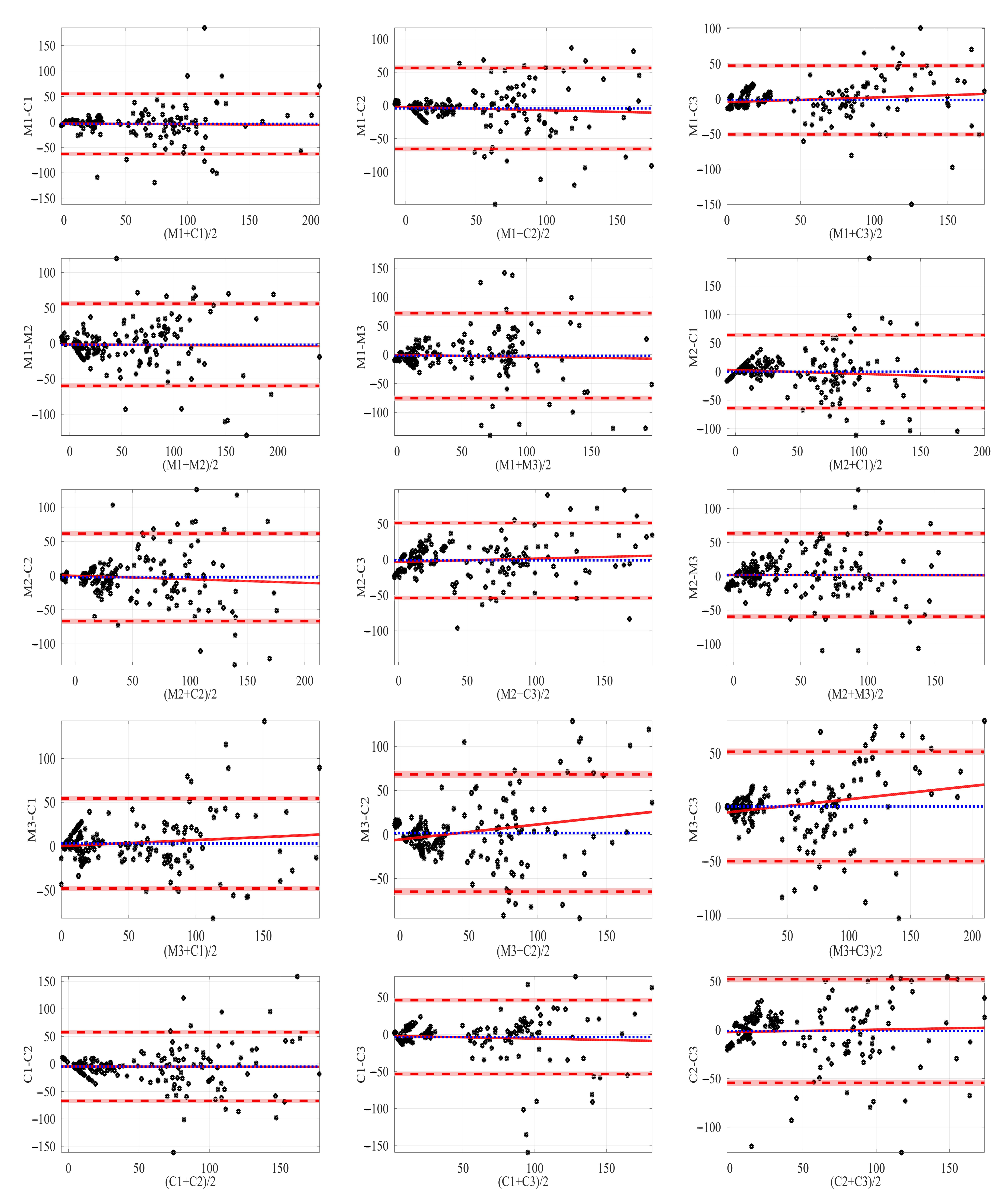
Bland–Altman plot indicates the average difference between the two readings. Figure 6 shows the Bland–Altman intra-operator reproducibility to Downs’ method.

The plots show all possible combinations between techniques and cases for Downs’ Cephalometric. As seen in Figure 6, the distribution is very similar to the example of the normal distribution shown in Figure 3.

Intra- and inter-operator were calculated for each case to Downs’ analysis, as shown in

Table 5. Difference Mean, Correlation Coefficient, Shapiro–Wilk test (W), and Repeatability coefficient ($RC$) of manually and software Downs’ technique.

Combination	Difference Mean	Correlation Coefficient	W	RC
Reproducibility (Intra-Operator)
M1-C1	−3.6932	−0.0201	0.7003	83.64
M2-C2	−2.6027	−0.0731	0.8709	90.76
M3-C3	0.6141	0.2277	0.8854	71.69
Reproducibility (Infra-Operator)
M1-M2	−1.1873	−0.0172	0.8862	81.98
M1-M3	−1.6729	−0.0394	0.8123	104.14
M1-C2	−4.45	−0.0670	0.8409	86.29
M1-C3	−1.7101	−0.4051	0.8411	69.2
M2-M3	1.8863	−0.0038	0.9039	86.82
M2-C1	−0.2242	−0.0910	0.8417	90.41
M2-C3	−1.3205	0.0855	0.9053	74.35
M3-C1	3.1618	0.1187	0.8692	72.49
M3-C2	1.6972	0.2227	0.8974	94.25
C1-C2	−4.8777	−0.0044	0.8398	88.1
C1-C3	−3.7398	−0.0648	0.7347	70.32
C2-C3	−1.1393	0.0432	0.8928	75.29

. Our observation clearly showed the low mean correlation (<0.6) for intra- and inter-operators reproducibility between all cases and techniques applications, showing the randomness between the measurements. Shapiro–Wilk test showed normal distribution (W close to 1) for intra- and inter-operators; this confirms the assumption was made previously.

The values of the repeatability coefficients are higher than the limit of 95% confidence interval showed for each combination in the Bland–Altman plot, as seen in Figure 6.

3.2.2. Steiner’s Cephalometric

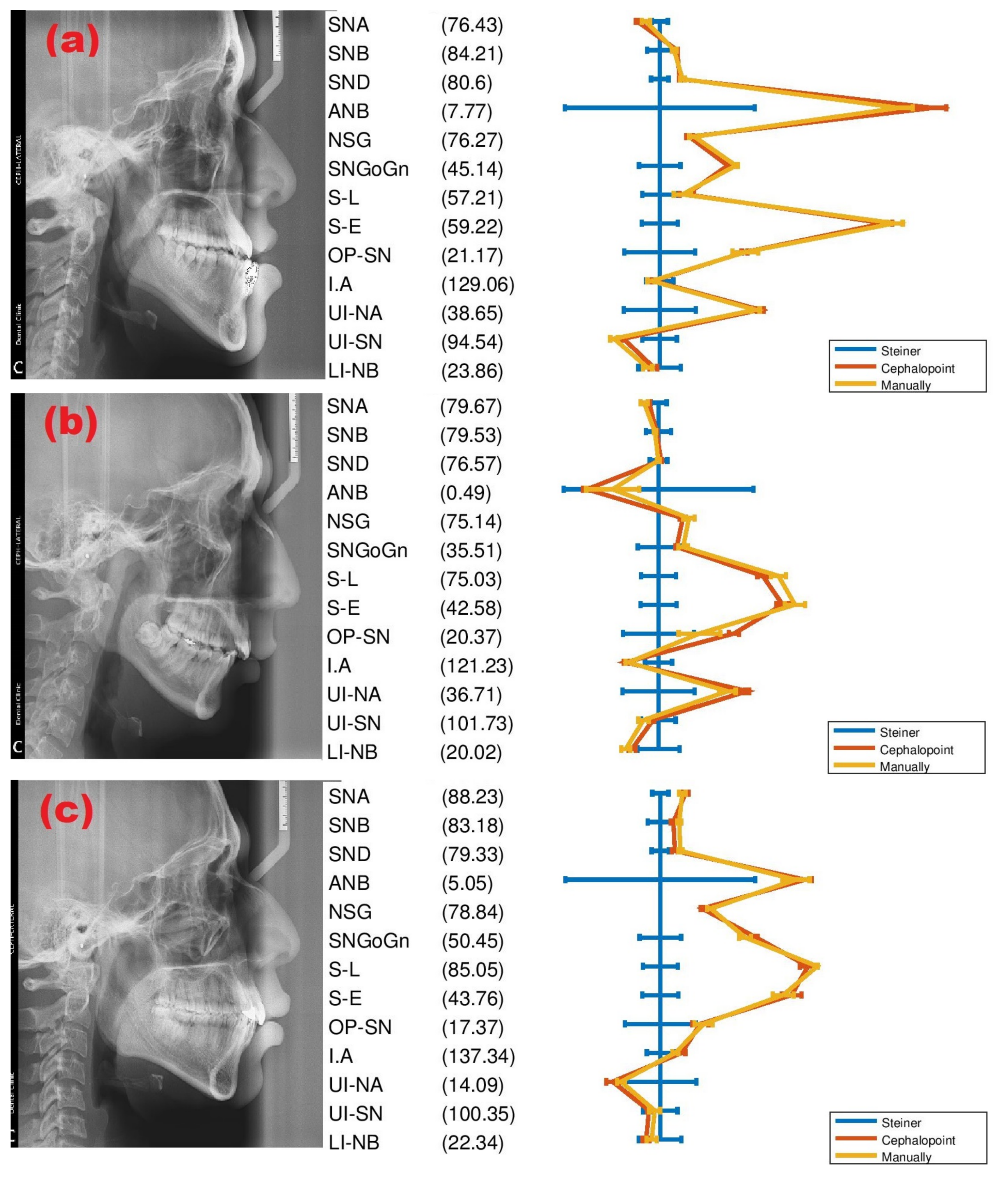
Case 1 (Figure 7a) was classified as Basifacial with the recessive location of the maxilla, mandibular prognathism, negative growth pattern, skeletal open bite case, class III skeletal tendency, and class III molar. Case 2 (Figure 7b) was classified as Dolichofacial with a negative growth pattern and class II div 1 dental case. Moreover, finally, case 3 (Figure 7c) is classified as Mesiofacial, class I skeletal tendency, and class I dental molar. These diagnostics were verified by applying Steiner’s conventional and digital techniques.

Three different cases were used to analyze Steiner’s Cephalometric, as shown in Figure 7. The 32 repetitions of each patient were necessary to estimate the mean of the variable and standard error, as shown in

Table 6. Steiner’s Lateral Cephalometric measurements for 3 different cases. The groups were classified in M (Manually) and C (Cephalopoint). Mean and standard error ($S_e$) were calculated for each variable.

Variable	Group	Case 1		Case 2		Case 3
		Mean	${\mathit{S}}_{\mathit{e}}$	Mean	${\mathit{S}}_{\mathit{e}}$	Mean	${\mathit{S}}_{\mathit{e}}$
SN-NA	M	$78.6°$	$\pm 1.0°$	$78.4°$	$\pm 0.85°$	$87.5°$	$\pm 0.8°$
	C	$76.4°$	$\pm 0.3°$	$79.7°$	$\pm 0.2°$	$88.2°$	$\pm 0.7°$
SN-NB	M	$83.4°$	$\pm 0.5°$	$79.1°$	$\pm 0.3°$	$84.6°$	$\pm 0.5°$
	C	$84.2°$	$\pm 0.2°$	$79.5°$	$\pm 0.2°$	$83.2°$	$\pm 0.7°$
SN-ND	M	$81.2°$	$\pm 0.6°$	$75.9°$	$\pm 0.4°$	$80.6°$	$\pm 0.5°$
	C	$80.6°$	$\pm 0.2°$	$76.6°$	$\pm 0.2°$	$79.3°$	$\pm 0.7°$
AN-NB	M	$7.1°$	$\pm 0.3°$	$1.0°$	$\pm 0.6°$	$4.9°$	$\pm 0.3°$
	C	$7.8°$	$\pm 0.3°$	$0.5°$	$\pm 0.1°$	$5.1°$	$\pm 0.2°$
NS-SGn	M	$77.3°$	$\pm 1.1°$	$76.4°$	$\pm 1.2°$	$80.7°$	$\pm 0.8°$
	C	$76.3°$	$\pm 0.7°$	$75.1°$	$\pm 0.6°$	$78.8°$	$\pm 0.4°$
SN-GoGn	M	$46.72°$	$\pm 0.4°$	$36.8°$	$\pm 0.9°$	$48.4°$	$\pm 1.1°$
	C	$45.1°$	$\pm 0.3°$	$35.5°$	$\pm 0.2°$	$50.5°$	$\pm 0.4°$
S-L	M	$56.3$ mm	$\pm 1.9$ mm	$78.6$ mm	$\pm 1.7$ mm	$87.2$ mm	$\pm 2.1$ mm
	C	$57.2$ mm	$\pm 1.6$ mm	$75.0$ mm	$\pm 1.2$ mm	$85.1$ mm	$\pm 1.9$ mm
S-E	M	$60.9$ mm	$\pm 1.3$ mm	$44.6$ mm	$\pm 1.7$ mm	$42.4$ mm	$\pm 1.7$ mm
	C	$59.2$ mm	$\pm 1.3$ mm	$42.6$ mm	$\pm 1.0$ mm	$43.8$ mm	$\pm 1.7$ mm
O.P.-SN	M	$21.2°$	$\pm 1.1°$	$17.5°$	$\pm 1.8°$	$17.7°$	$\pm 0.8°$
	C	$21.2°$	$\pm 0.3°$	$20.4°$	$\pm 0.4°$	$17.4°$	$\pm 0.7°$
I.A.	M	$128.6°$	$\pm 1.2°$	$122.2°$	$\pm 0.9°$	$135.5°$	$\pm 0.9°$
	C	$129.1°$	$\pm 0.6°$	$121.2°$	$\pm 0.5°$	$137.3°$	$\pm 1.1°$
U.I.-NA	M	$37.9°$	$\pm 0.7°$	$33.5°$	$\pm 1.3°$	$15.5°$	$\pm 0.7°$
	C	$38.7°$	$\pm 0.5°$	$36.7°$	$\pm 0.3°$	$14.1°$	$\pm 1.1°$
U.I.-SN	M	$92.3°$	$\pm 0.9°$	$99.5°$	$\pm 1.2°$	$101.7°$	$\pm 1.3°$
	C	$94.5°$	$\pm 0.4°$	$101.7°$	$\pm 0.2°$	$100.4°$	$\pm 0.4°$
L.I.-NB	M	$22.7°$	$\pm 0.9°$	$18.8°$	$\pm 0.9°$	$23.4°$	$\pm 0.9°$
	C	$23.9°$	$\pm 0.7°$	$20.0°$	$\pm 0.7°$	$22.3°$	$\pm 0.7°$

.

As seen in Table 6, Steiner’s Cephalometric measurements obtained manually and software technique were very close. The mean absolute error (MAE) was calculated like Downs’ Cephalometric cases. The MAE estimated for the manual technique was 5.04%, while the software technique was 3.72%.

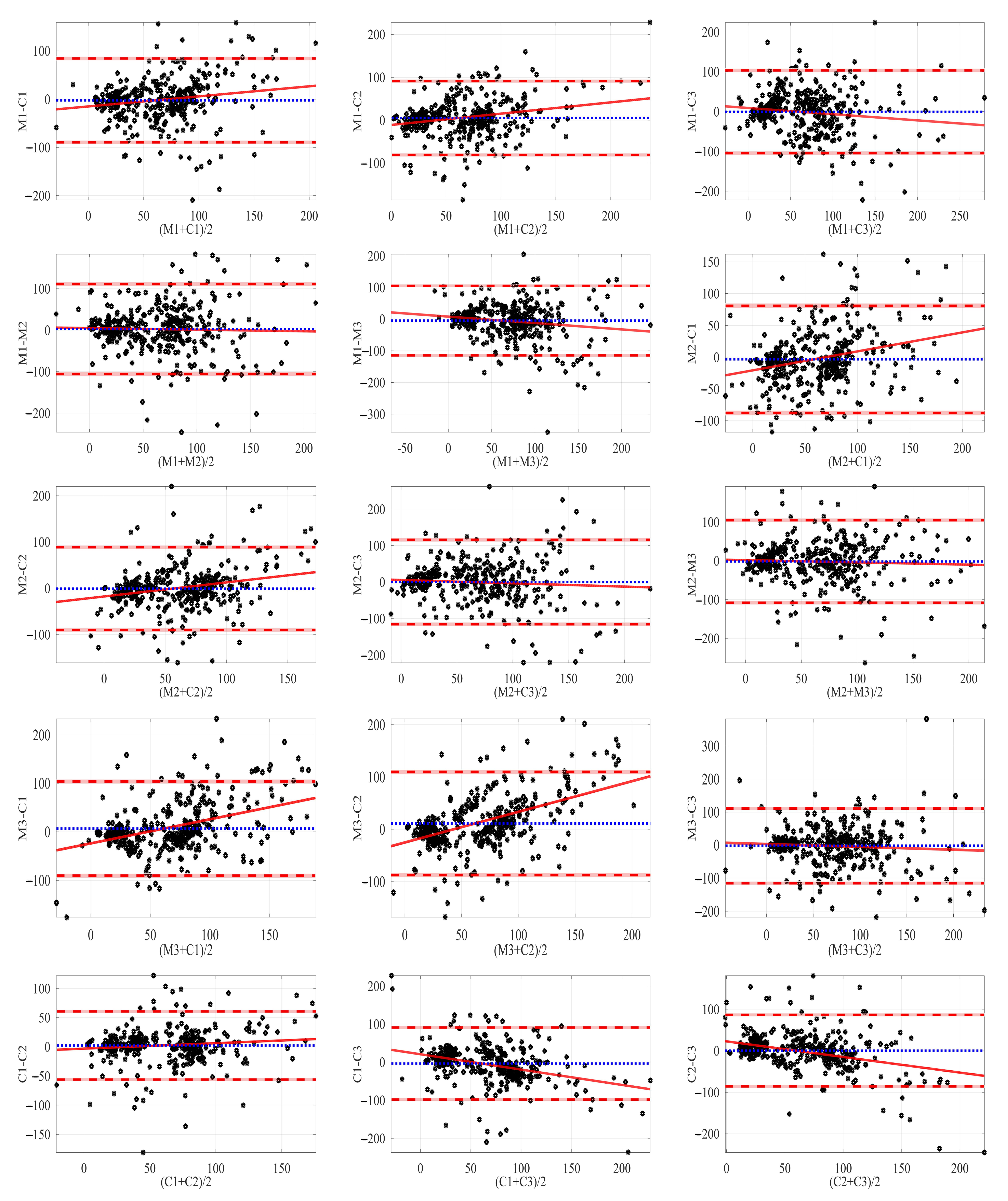
Bland–Altman analysis was also employed with Steiner’s Cephalometric measurements. The Bland–Altman plots intra-operator reproducibility to Steiner’s method are shown in Figure 8.

As expected, the plots show all possible combinations between techniques and cases for Steiner’s Cephalometric. As seen in Figure 8, the normal distribution in all Bland–Altman plots is very clear.

Intra- and inter-operator were calculated for each case to Steiner’s analysis, as shown in Figure 8. Our observation demonstrated the low mean correlation (>0.6) between intra- and inter-operator reproducibility for all cases and techniques applications, showing the randomness between the measurements. Shapiro–Wilk test showed normal distribution (W close to 1) for intra- and inter-operators; this confirms the assumption was made previously, as seen in

Table 7. Difference Mean, Correlation Coefficient, Shapiro–Wilk test (W), and Repeatability coefficient (RC) of manually and software Steiner’s technique.

Combination	Difference Mean	Correlation Coefficient	W	RC
Reproducibility (Intra-Operator)
M1-C1	−2.6614	0.1828	0.9256	123.01
M2-C2	−0.7623	0.2521	0.9052	126.41
M3-C3	−2.0150	−0.071	0.8941	159.89
Reproducibility (Infra-Operator)
M1-M2	2.5761	−0.0292	0.9274	153.28
M1-M3	−4.7254	−0.1640	0.8918	155.31
M1-C2	5.0451	0.2459	0.9206	121.79
M1-C3	−0.4968	−0.1375	0.9577	147.09
M2-M3	−1.6137	−0.0482	0.9106	150.49
M2-C1	−3.3997	0.2925	0.9490	119.24
M2-C3	0.1517	−0.0691	0.9295	163.67
M3-C1	6.6871	0.4232	0.8997	137.39
M3-C2	11.0084	0.5190	0.9230	139.27
C1-C2	0.0327	−0.3764	0.9002	82.53
C1-C3	−3.5717	−0.3607	0.9026	129.17
C2-C3	0.3883	−0.3628	0.8745	121.92

.

The values of the repeatability coefficients are higher than the limit of 95% confidence interval showed for each combination in the Bland–Altman plot, as seen in Figure 8.

3.3. Statistical Test

The mean, standard deviation, kurtosis, p-value, and Shapiro–Wilk test were the statistical variables calculated for each Cephalometric method applying Cephalopoint.

3.3.1. Downs’ Cephalometric

A group of 42 patients (18 M, 24 F); mean age $13\pm 5$; ranging from 7 to 19 years were measured using Downs’ Cephalometric and analyzed using statistical variables.

All variables of Downs’ Cephalometric were non statistically significant difference $p>0.05$, in combination with $W\approx 1$, as seen in

Table 8. Downs’ Lateral Cephalometric measures employing Cephalopoint and statistical analysis. Mean (m), standard deviation (S), excess kurtosis ($K_e$), lower limit ($LL$), p-value (p), upper limit ($UL$), and Shapiro–Wilk test (W) were calculated.

	m	S	LL	${\mathit{K}}_{\mathit{e}}$	UL	p	W
PoOr-NPg	83.11$°$	±4.50	−1.6190	1.1734	1.6190	0.0524	0.9475
Na-A-Pg	10.02$°$	±5.32	−0.4618	−0.1085	0.4618	0.0557	0.9482
AB-NPg	−5.67$°$	±3.85	−0.1724	−0.1631	0.1724	0.6420	0.9795
PoOr-GoMe	36.43$°$	±6.60	−0.3087	0.2277	0.3087	0.9105	0.9871
SGn-PoOr	111.35$°$	±5.43	−1.2441	1.1876	1.2441	0.1288	0.9583
PoOr-OP	15.44$°$	±6.40	−0.9737	0.5170	0.9737	0.3129	0.9693
I.A.	118.81$°$	±7.74	−0.5360	−0.3289	0.5360	0.4301	0.9735
L.I.-OP	21.45$°$	±5.70	−0.2056	−0.0917	0.2056	0.7213	0.9815
L.I.-GoMe	89.54$°$	±6.03	−1.1388	0.0058	1.1388	0.2045	0.9640
U.I.-APg	9.02 mm	±3.89	−0.2189	−0.0753	0.2189	0.9890	0.9918

, the variables showed normal distribution. After analyzing the excess kurtosis, all the variables exhibited Mesokurtic distribution ($LL<K_e<UL$), confirming normally distributed measurements.

3.3.2. Steiner’s Cephalometric

A group of 42 patients (20 M, 22 F); mean age $54\pm 12$; ranging from 20 to 72 years were measured using Steiner’s Cephalometric and analyzed using statistical variables.

All variables of Steiner’s Cephalometric were non statistically significant difference $p>0.05$, in combination with $W\approx 1$, as seen in

Table 9. Steiner’s Lateral Cephalometric measures employing Cephalopoint and statistical analysis. Mean (m), standard deviation (S), excess kurtosis ($K_e$), lower limit ($LL$), p-value (p), upper limit ($UL$), and Shapiro–Wilk test (W) were calculated.

	m	S	LL	${\mathit{K}}_{\mathit{e}}$	UL	p	W
SN-NA	87.29$°$	±6.14	−0.2854	0.2705	0.2854	0.8218	0.9830
SN-NB	83.03$°$	±4.51	−0.1405	−0.0185	0.1405	0.6802	0.9789
SN-ND	77.17$°$	±4.80	−0.5109	−0.2248	0.5109	0.3170	0.9670
AN-NB	4.84$°$	±2.90	−1.0293	−0.7372	1.0293	0.0699	0.9468
NS-SGn	69.92$°$	±4.92	−1.3503	−0.3865	1.3503	0.1740	0.9250
SN-GoGn	42.45$°$	±9.65	−1.6985	0.7451	1.6985	0.5432	0.9404
S.L.	57.00 mm	±14.17	−0.4324	−0.1538	0.4324	0.7140	0.9799
S.E.	29.51 mm	±6.15	−1.8500	1.2561	1.8500	0.0533	0.9404
O.P.-SN	16.39$°$	±6.05	−0.0900	−0.0415	0.0900	0.9202	0.9865
I.A.	117.02$°$	±10.32	−1.1567	0.2280	1.1567	0.3270	0.9674
U.I.-NA	27.60$°$	±7.69	−1.5263	0.8537	1.5263	0.2062	0.9611
U.I.-SN	114.89$°$	±7.95	−0.9395	−0.2570	0.9395	0.3659	0.9690
L.I.-NB	14.54$°$	±5.72	−1.1434	0.2292	1.1434	0.4287	0.9713

, the variables showed normal distribution. After analyzing the excess kurtosis, all the variables exhibited Mesokurtic distribution ($LL<K_e<UL$), confirming normally distributed measurements.

4. Discussion

Cephalopoint could significantly reduce the time employed by the dentist to analyze the Cephalograms. In this sense, the diagnostic would be almost instantly, and the clinics will be more efficient. On the other hand, if campaign programs in low-income communities where the provisional clinic would be installed, electric energy will be necessary.

The mobility could be improved by applying the same principles to create a mobile application. Thus, these clinical campaign programs would be expanded to the most remote communities.

These codes would be migrated to another programming language like Python, offering the advance of not needing software, like Octave, to run each code. Furthermore, Phyton offers the possibility to improve the graphic interface to be more friendly.

On the other hand, Octave is the programming language more used by the Mathematics Academy of Engineering Faculty members, prioritizing that other researchers, teachers, and students can join the project to improve it. Several routines on Octave and Python were running and compared, and both were very similar in precision and time employed [24,25]. Both languages are excellent open source alternatives.

Cephalopoint was designed to offer a free alternative to analyze with Downs’ and Steiner’s Cephalometric techniques. The use of open source software has several advantages. Other users could modify it to their specific needs, either working with Cephalometrics or analyzing further X-ray radiographs. Both the interface and the code are constantly evolving thanks to the internet community. The success of open source software development has increased the number of companies seeking this development model. Many software companies have approached the open source software community to work collaboratively to increase the use of these programs [26].

Cephalopoint could be improved by adding a routine to compare the measurements with the standard values for each variable and return the difference. Another to plot the Cephalometric points and planes instantly after was declared. The use of filters to clean up the image could improve the selection of Cephalometric points.

The image analysis techniques on the Cephalograms will be applied to recognize patterns and thus detect the different landmarks of each Cephalometric method. A first approximation could be applying an artificial neural network to acknowledge texture characterization as Fibrosis and Carcinoma in lungs [27], in the same way, we will seek to recognize the Cephalometric landmarks.

The same analysis to calculate the angles and distances between the reference points could be used in other fields of medicine, where the study of radiographs is involved. For example, to study bone thickness in magnetic resonance imaging of bodies postoperative vertebrae L4 and L5, using the proposed technique to evaluate the treatment of pyogenic spondylodiscitis [28]. To measure the angle of pelvic tilt in sagittal radiograph to determine the evolution of scoliosis deterioration [29]. Furthermore, to offer an alternative software to measure the orbital volume after Enucleation with Orbital Implant [30].

Many studies compared the manual with digital lateral Cephalometric using license software. Bastos Paixão et al. employed Dolphin and analyzed with t-Student distribution [31], Thurzo et al. employed Dolphin and analyzed with Bland–Altman analysis. Esteva Segura et al. [32] employed Nemoceph Nx and analyzed with t-student distribution [33], Gartati et al. employed CephNinja and analyzed with t-Student distribution [8], Mohan et al. employed OneCeph and analyzed with t-students distribution [34], among other authors. All the studies confirmed no significant differences and normal distribution for all Cephalometric variables measured by software. Furthermore, the error standard of each variable was reduced, exhibiting the argument of Alburquerque-Junior and Almeida [35] and Chen et al. [36]: “the computerized method is reliable as it exhibits lower error variance than the conventional method”. In the present document, both issues were confirmed by applying open source software of own design.

5. Conclusions

Cephalopoint could be offered some advances and problems compared with other commercial software. However, this software is not trying to compete but offers a low-income alternative with good accuracy and repeatability.

The average time employed to do Cephalometric analysis with the software was reduced to the third part concerning manual technique. The measurements were calculated almost in an average time of 6 min. Thus, the software could help the dentist reduce the time required to perform a diagnostic.

On the other hand, using the file where all the measurements are saved reduces the time to carry out statistical studies and organize patient information. Furthermore, the CSV format creates universal files that could be worked in any spreadsheet or statistical software.

Another advantage of the software is the appreciable decrease in error measurement considering the manual technique in Down’s method from 6.73% to 4.73% and Steiner’s method from 5.04% to 3.72%, which was to be expected as commented in the previous section.

Table 5 and Table 7 show the comparison with the manual and software technique using the Bland–Altman analysis. It exhibited that for both the Downs and Steiner methods, the correlation is very low, so it can be considered that the measurements in the different cases are entirely independent of each other. The Down’s method ($W>0.7$) and Steiner’s method ($W>0.87$) were calculated using the Shapiro–Wilk test; in both, the behavior of all different combinations of differences between measurements and cases, in other words, the infra- and intra-operators have a normal distribution. This assumption was confirmed in Bland–Altman plots, as seen in Figure 6 to Downs’ technique and Figure 8 to Steiner’s technique.

The repeatability of each case analyzed by Down’s and Steiner’s methods applying Cephalopoint was very high, as seen in Table 5 and Table 7.

About statistical analysis, all the variables analyzed Down’s and Steiner’s methods applying Cephalopoint showed normal distribution, as seen in Table 8 and Table 9. Consequently, the measurements obtained did not present statistical biases, so Cephalopoint is a good instrument for clinical statistical analysis.

The free software designed, Cephalopoint, is a good instrument to apply Down’s and Steiner’s Cephalometric methods, exhibiting enough accuracy, precision, and repeatability, with the possibility to be employed for clinical studies. It adds one more possibility to the list of software that can perform this type of measurement.

References

1. Steiner, C.C. Cephalometrics for you and me. Am. J. Orthod. 1953, 39, 729–755. [Google Scholar] [CrossRef]
2. Betanzo Astudillo, L. Manual de Anatomía Radiográfica y Cefalometría Básica; Departamento de Pediatría Bucal, Facultad de Odontología, Universidad de Concepción: Concepción, Chile, 2013. [Google Scholar]
3. Pradip, S.; Harish Kumar, S.; Om Prakash, K.; Ritu, D. Comparison of reliability and validity of posteroanterior cephalometric measurements obtained from AutoCEPH© and dolphin® cephalometric software programs with manual tracing. J. Indian Orthod. Soc. 2018, 52, 106–114. [Google Scholar]
4. Erkan, M.; Gurel, H.G.; Nur, M.; Demirel, B. Reliability of four different computerized cephalometric analysis programs. Eur. J. Orthod. 2012, 34, 318–321. [Google Scholar] [CrossRef] [PubMed] [Green Version]
5. Nimkarn, Y.; Miles, P. Reliability of computer-generated cephalometrics. Int. J. Adult Orthod. Orthognath. Surg. 1995, 10, 43–52. [Google Scholar]
6. Roden-Johnson, D.; English, J.; Gallerano, R. Comparison of hand-traced and computerized cephalograms: Landmark identification, measurement, and superimposition accuracy. Am. J. Orthod. Dentofac. Orthop. 2008, 133, 556–564. [Google Scholar] [CrossRef] [PubMed]
7. Perrotti, G.; Baccaglione, G.; Clauser, T.; Scaini, R.; Grassi, R.; Testarelli, L.; Reda, R.; Testori, T.; Del Fabbro, M. Total Face Approach (TFA) 3D Cephalometry and Superimposition in Orthognathic Surgery: Evaluation of the Vertical Dimensions in a Consecutive Series. Methods Protoc. 2021, 4, 36. [Google Scholar] [CrossRef]
8. Gita, G.; Andriani, H.; Yuliawati, Z.; Iwa Rahmat, S. Steiner cephalometric analysis discrepancies between conventional and digital methods using Cephninja® application software. Padjadjaran J. Dent. 2016, 28. [Google Scholar] [CrossRef] [Green Version]
9. World Health Organization; The World Bank. Tracking Universal Health Coverage: 2017 Global Monitoring Report; World Health Organization: Geneva, Switzerland, 2017; pp. 14–69. [Google Scholar]
10. Downs, W.B. The role of cephalometrics in orthodontic case analysis and diagnosis. Am. J. Orthod. 1952, 38, 162–182. [Google Scholar] [CrossRef]
11. De Oca, C.; Zamora, C. Compendio de Cefalometría; Amolca: Ciudad de México, México, 2010. [Google Scholar]
12. Reyes Salgado, J. Cephalopoint. Available online: https://sites.google.com/upaep.mx/cephalopoint (accessed on 16 November 2021).
13. Giavarina, D. Understanding Bland Altman analysis. Biochem. Medica 2015, 25, 141–151. [Google Scholar] [CrossRef] [Green Version]
14. Bland, M. An Introduction to Medical Statistics/Martin Bland, 3rd ed.; Oxford University Press: New York, NY, USA, 2000; pp. 13, 365. [Google Scholar]
15. Bland, J.; Altman, D. Statistical methods for assessing agreement between two methods of clinical measurement. Int. J. Nurs. Stud. 2010, 47, 931–936. [Google Scholar] [CrossRef]
16. Kenton, W. Kurtosis. Available online: https://www.investopedia.com/terms/k/kurtosis.asp (accessed on 19 November 2021).
17. Gawali, S. Shape of Data: Skewness and Kurtosis. Available online: https://www.analyticsvidhya.com/blog/2021/05/shape-of-data-skewness-and-kurtosis/ (accessed on 20 November 2021).
18. Doane, D.P.; Seward, L.E. Measuring Skewness: A Forgotten Statistic? J. Stat. Educ. 2011, 19, 2. [Google Scholar] [CrossRef]
19. Glen, S. Shapiro–Wilk Test: What It Is and How to Run It. Available online: https://www.statisticshowto.com/shapiro-wilk-test/ (accessed on 20 November 2021).
20. Davis, C.S.; Stephens, M.A. The covariance matrix of normal order statistics. Commun. Stat. Simul. Comput. 1977, 6, 75–81. [Google Scholar] [CrossRef]
21. Krakauer, N. Shapiro–Wilk Test in Octave. Available online: https://gist.github.com/nir-krakauer/7d308d1501bf2d07b30eb4a9a3afbd0a (accessed on 21 November 2021).
22. Royston, P. Approximating the Shapiro–Wilk W-test for non-normality. Stat. Comput. 1992, 2, 117–119. [Google Scholar] [CrossRef]
23. Shapiro, S.S.; Wilk, M.B. An Analysis of Variance Test for Normality (Complete Samples). Biometrika 1965, 52, 591–611. [Google Scholar] [CrossRef]
24. Guedes, P.F.S.; Nepomuceno, E.G. Some remarks on the performance of Matlab, Python and Octave in simulating dynamical systems. arXiv 2019, arXiv:1910.06117. [Google Scholar]
25. Chaves, J.C.; Nehrbass, J.; Guilfoos, B.; Gardiner, J.; Ahalt, S.; Krishnamurthy, A.; Unpingco, J.; Chalker, A.; Warnock, A.; Samsi, S. Octave and Python: High-Level Scripting Languages Productivity and Performance Evaluation. In Proceedings of the 2006 HPCMP Users Group Conference (HPCMP-UGC’06), Denver, CO, USA, 26–29 June 2006; pp. 429–434. [Google Scholar] [CrossRef]
26. Daniel, S.L.; Maruping, L.M.; Cataldo, M.; Herbsleb, J. The impact of ideology misfit on open source software communities and companies. Manage. Inf. Syst. Q. 2018, 42, 1069–1096. [Google Scholar] [CrossRef]
27. Devan, L.; Santosham, R.; Hariharan, R. Automated Texture-Based Characterization of Fibrosis and Carcinoma Using Low-Dose Lung CT Images. Int. J. Imaging Syst. Technol. 2014, 24, 39–44. [Google Scholar] [CrossRef]
28. Pola, E.; Autore, G.; Formica, V.M.; Pambianco, V.; Colangelo, D.; Cauda, R.; Fantoni, M. New classification for the treatment of pyogenic spondylodiscitis: Validation study on a population of 250 patients with a follow-up of 2 years. Eur. Spine J. 2017, 26, 479–488. [Google Scholar] [CrossRef]
29. Haaker, G.; Forst, J.; Forst, R.; Fujak, A. Orthopedic management of patients with Pompe disease: A retrospective case series of 8 patients. Sci. World J. 2014, 2014, 963861. [Google Scholar] [CrossRef]
30. Lukats, O.; Vízkelety, T.; Markella, Z.; Maka, E.; Kiss, M.; Dobai, A.; Bujtár, P.; Szucs, A.; Barabas, J. Measurement of Orbital Volume after Enucleation and Orbital Implantation. PLoS ONE 2012, 7, e50333. [Google Scholar] [CrossRef]
31. Abreu, D.; Freitas, K.M.; Nomura, S.; Valarelli, F.; Cançado, R. Comparison among manual and computerized cephalometrics using the softwares dolphin imaging and dentofacial planner. Dent. Oral Craniofacial Res. 2016, 2, 6. [Google Scholar] [CrossRef]
32. Thurzo, A.; Javorka, V.; Stanko, P.; Lysý, J.; Suchancova, B.; Lehotska, V.; Valkovic, L.; Makovnik, M. Digital and manual cephalometric analysis. Bratisl. Lekárske Listy 2010, 111, 97–100. [Google Scholar]
33. Segura, F.; Valverde, A.; Melendez, A.; Angelares, P. Comparative study between digital and manual cephalometry with digital radiographs. Rev. Mex. Ortod. 2014, 2, e93–e96. [Google Scholar] [CrossRef] [Green Version]
34. Mohan, A.; Sivakumar, A.; Nalabothu, P. Evaluation of accuracy and reliability of OneCeph digital cephalometric analysis in comparison with manual cephalometric analysis—A cross-sectional study. BDJ Open 2021, 7, 22. [Google Scholar] [CrossRef]
35. Albuquerque Junior, H.R.D. Avaliação do erro de reprodutibilidade dos valores cefalométricos aplicados na filosofia Tweed-Merrifield, pelos métodos computadorizado e convencional. Ortodontia 1998, 31, 19–30. [Google Scholar]
36. Chen, Y.J.; Chen, S.; Chang, H.; Chen, K.j. Comparison of Landmark Identification in Traditional Versus Computer-Aided Digital Cephalometry. Angle Orthod. 2000, 70, 387–392. [Google Scholar] [CrossRef]
37. Eck, D.J. Introduction to Computer Graphics, 12th ed.; Hobart and William Smith Colleges: Geneva, NY, USA, 2018. [Google Scholar]
38. Lavin, L. Radiography in Veterinary Technology—E-Book; Elsevier Health Sciences: Amsterdam, The Netherlands, 2006. [Google Scholar]
39. Grossman, S. Álgebra Lineal; Elibro Catedra, McGraw-Hill Interamericana de España S.L.: New York, NY, USA, 2008. [Google Scholar]
Figure 1. Lateral Cephalometric reference landmarks: Nasion (N), Sella (S), A point (A), B point (B), D point (D), Gonion (Gon), Menton (Me), Pogonion (Pg), Gnathion (Gn), Porion (Po) and Infraorbital (Or). Planes and angles: Occlusal Plane (O.P.) and Incisor Angle (I.A.).
Digital 02 00008 g001
Figure 2. Flowchart diagram (left size) and graphic interface (right size) of Cephalopoint.
Digital 02 00008 g002
Figure 3. (a). Bland–Altman plot of two methods with good agreement. The horizontal blue dotted line represents the mean difference between the two methods, the horizontal red dotted line the limits of agreement, and the solid red regression line of confidence interval limit. (b). Distribution plot of differences between measurement by methods A and B. The red line represents a normal distribution.
Digital 02 00008 g003
Figure 4. (a). Leptokurtic distribution. (b). Mesokurtic distribution. (c). Platykurtic distribution.
Digital 02 00008 g004
Figure 5. Cephalometric (a) Case 1. (b) Case 2, and (c) Case 3 analyzed by Downs’ technique. The lateral radiographs are shown on the left side; meanwhile, Downs’ polygons are on the right side. In Downs’ polygons, the blue line represents the typical values for Downs. As shown in Table 1, the red line is the average and standard error calculated by Cephalopoint, and the yellow line is the average and standard error manually calculated. The number between parentheses was the value calculated by Cephalopoint.
Digital 02 00008 g005
Figure 6. The Bland–Altman plot intra-operator reproducibility to Downs’ Cephalometric. Comparative between manual and software techniques for three cases.
Digital 02 00008 g006
Figure 7. Cephalometric (a) Case 1. (b) Case 2, and (c) Case 3 analyzed by Steiner’s technique. The lateral radiographs are shown on the left side and Steiner’s polygons on the right side. In Steiner’s polygons, the blue line represents the typical values for Steiner. As shown in Table 2, the red line is the average and standard error calculated by Cephalopoint, and the yellow line is the average and standard error manually calculated. The number between parentheses was the value calculated by Cephalopoint.
Digital 02 00008 g007
Figure 8. The Bland–Altman plot intra-operator reproducibility to Steiner’s Cephalometric. Comparative between manual and software techniques for three cases.
Digital 02 00008 g008