
In Vivo Dosimetry for Superficial High Dose Rate Brachytherapy with Optically Stimulated Luminescence Dosimeters: A Comparison Study with Metal-Oxide-Semiconductor Field-Effect Transistors

Abstract
Simple Summary
Abstract
1. Introduction
2. Materials and Methods
2.1. Calibration
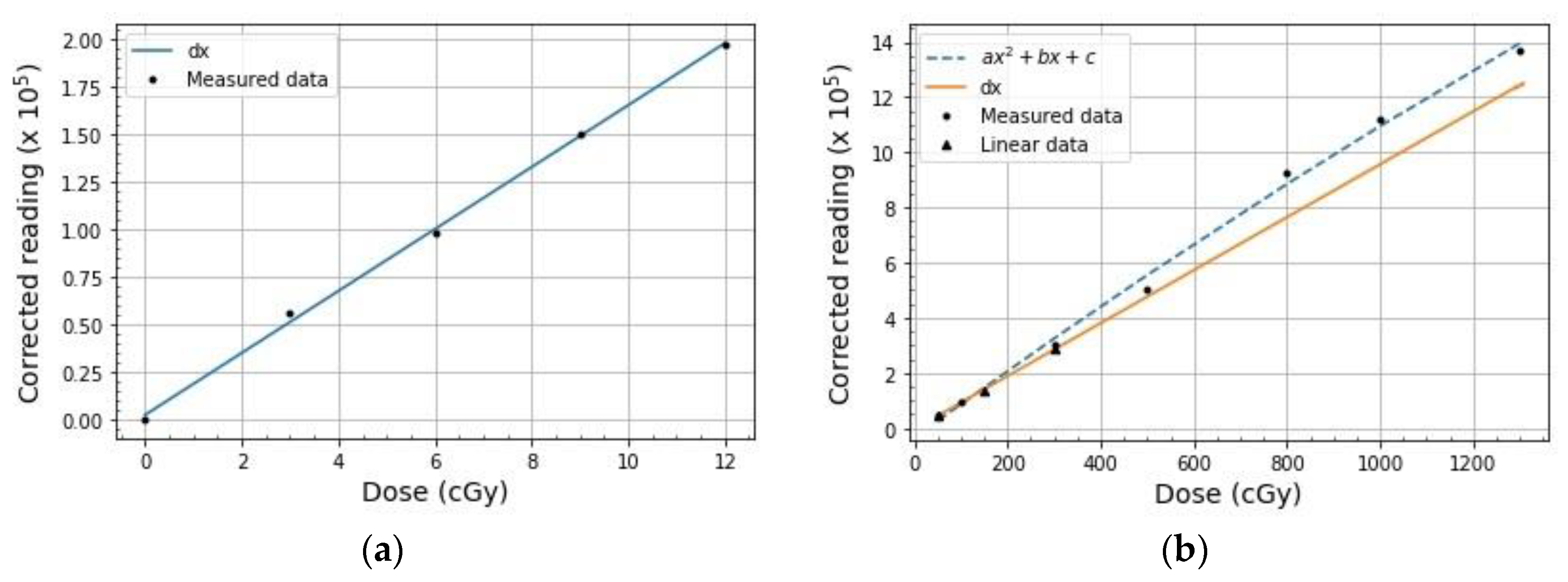
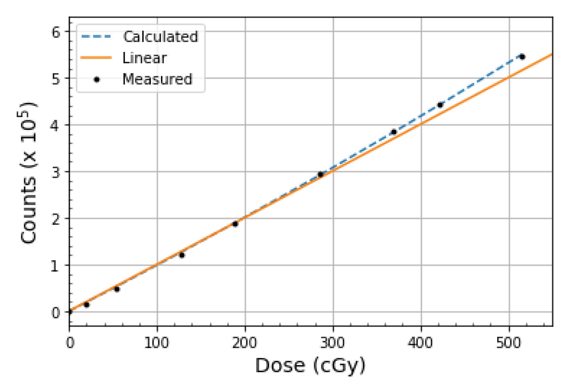
2.2. Dose Linearity
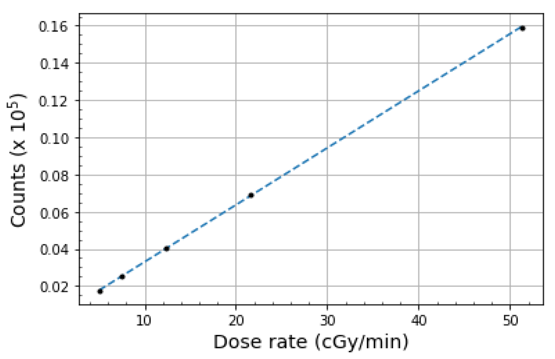
2.3. Dose Rate Dependence
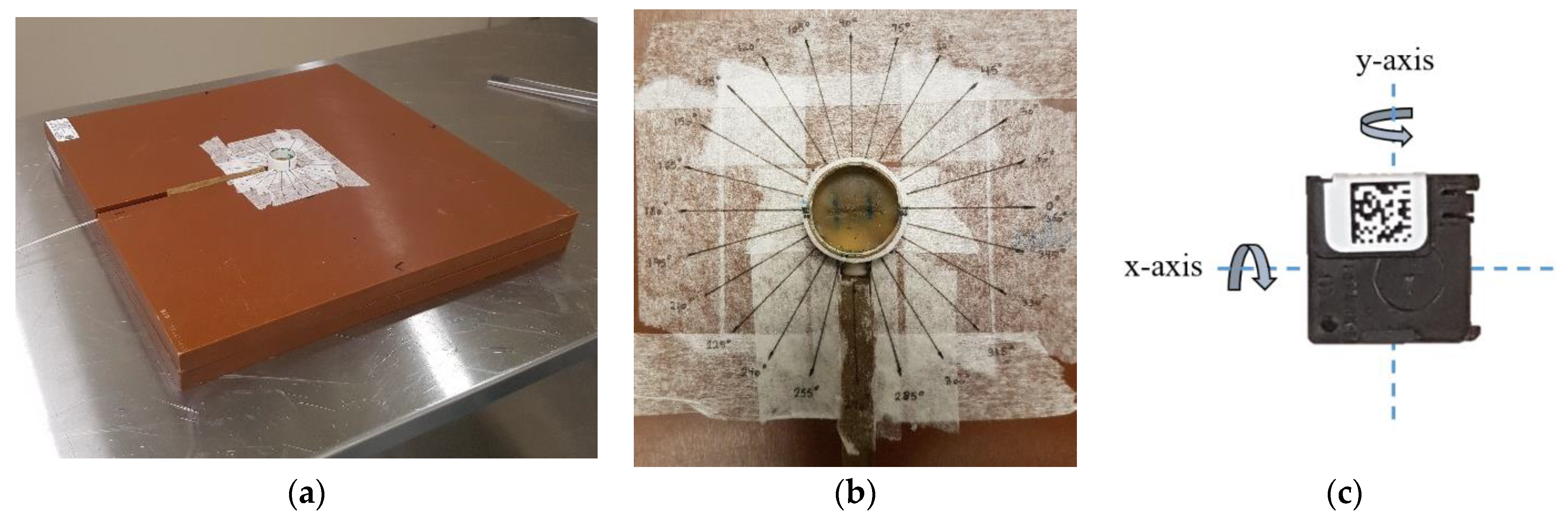
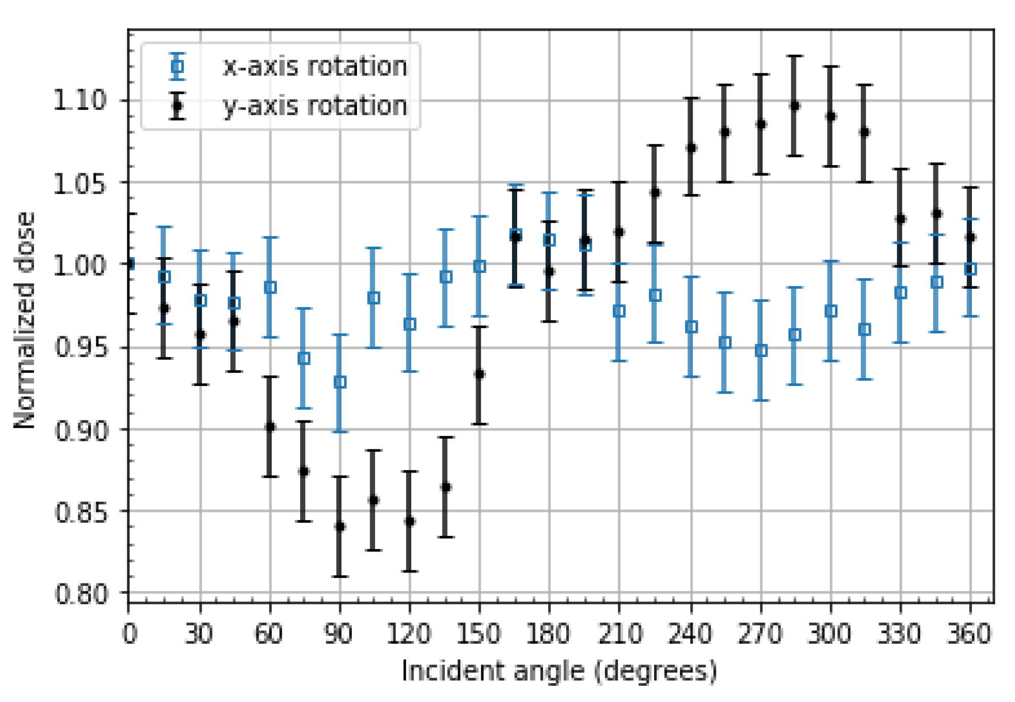
2.4. Angular Dependence
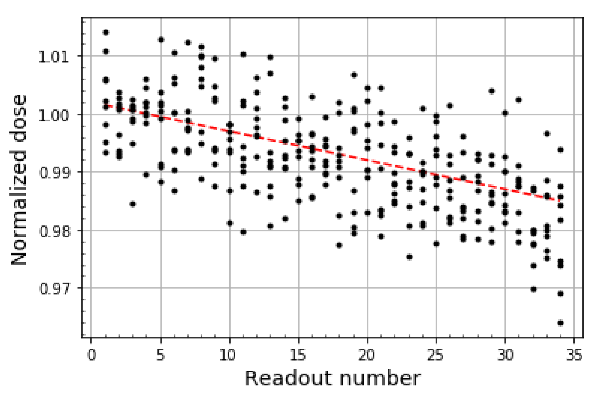
2.5. Readout Depletion
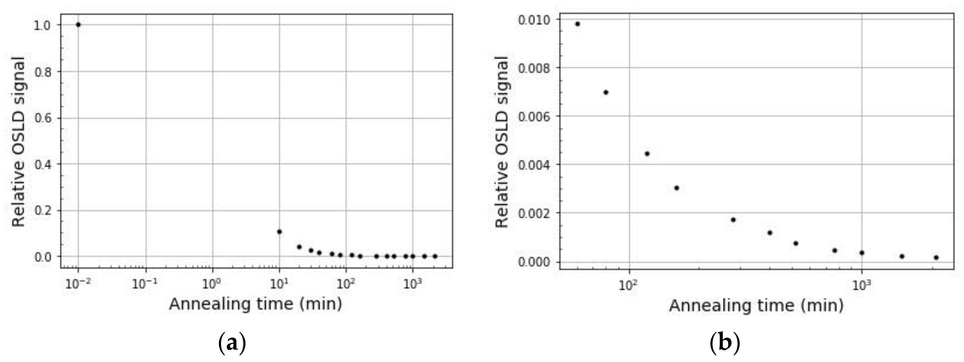
2.6. Optical Annealing
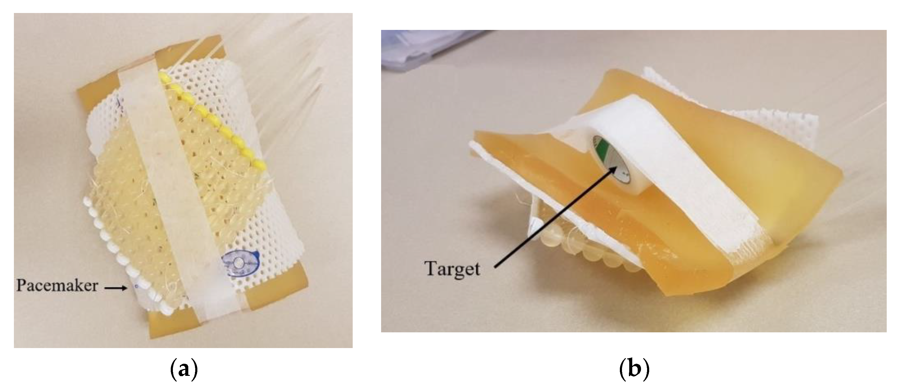
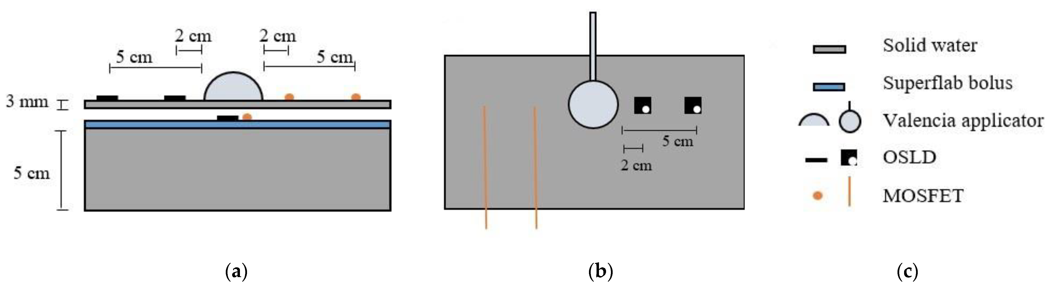
2.7. End-to-End Testing
3. Results
3.1. Calibration
3.2. Dose Linearity
3.3. Dose Rate Dependence
3.4. Angular Dependence
3.5. Readout Depletion
3.6. Optical Annealing
3.7. End-to-End Testing
4. Discussion
4.1. Calibration
4.2. Dose Linearity
4.3. Dose Rate Dependence
4.4. Angular Dependence
4.5. Readout Depletion
4.6. Optical Annealing
4.7. End-to-End Testing
4.8. OSLDs vs. MOSFETs: Clinical Relevance
5. Conclusions
- Use of screened nanoDotsTM is recommended for building calibration curves.
- The appropriate calibration must be selected before measurement.
- Using a weak beam of light, OSLDs exhibit minimal signal depletion with multiple readouts (−0.05% per readout).
- OSLDs exhibit angular dependence in edge-on cases which are 90° ± 30° and 270° ± 30° in incident angle. It is recommended to place OSLDs orthogonal or near orthogonal to the expected incident dose gradient to prevent angular dependence and volume-averaging corrections during readout.
- Optical annealing of OSLDs is a viable way to reuse OSLDs for clinical and research purposes, permitting a baseline measurement to be made after the annealing period and before the next irradiation.
- Using the light source described in this paper, OSLDs must be optically annealed for a minimum of 24 h and subsequently kept in the dark for a minimum of four minutes prior to a baseline readout.
- Precise comparisons of OSLD, MOSFET, and TPS point doses are only recommended when OSLDs and MOSFETs are positioned in low-dose gradient regions or when the OSLD irradiation geometry closely matches the geometry of the tissue of interest. Otherwise, very large discrepancies are to be expected due to positional uncertainties.
- In vivo dose measurements can successfully be made.
Supplementary Materials
Author Contributions
Funding
Institutional Review Board Statement
Informed Consent Statement
Data Availability Statement
Acknowledgments
Conflicts of Interest
References
- Apalla, Z.; Lallas, A.; Sotiriou, E.; Lazaridou, E.; Ioannides, D. Epidemiological trends in skin cancer. Derm. Pr. Concept. 2017, 7, 1–6. [Google Scholar] [CrossRef] [PubMed]
- Centers for Disease Control and Prevention. Kinds of Cancer. Available online: https://www.cdc.gov/cancer/kinds.htm (accessed on 3 July 2022).
- Government of Canada. Non Melanoma Skin Cancer. Available online: https://www.canada.ca/en/public-health/services/chronic-diseases/cancer/non-melanoma-skin-cancer.html (accessed on 3 July 2022).
- Griffin, L.L.; Ali, F.R.; Lear, J.T. Non-melanoma skin cancer. Clin. Med. J. 2016, 16, 62–65. [Google Scholar] [CrossRef] [PubMed]
- Fahradyan, A.; Howell, A.C.; Wolfswinkel, E.M.; Tsuha, M.; Sheth, P.; Wong, A.K. Updates on the management of non-melanoma skin cancer (NMSC). Healthcare 2017, 5, 82. [Google Scholar] [CrossRef]
- Taylor, J.M.; Dasgeb, B.; Liem, S.; Ali, A.; Harrison, A.; Finkelstein, M.; Cha, J.; Anne, R.; Greenbaum, S.; Sherwin, W.; et al. High-dose-rate brachytherapy for the treatment of basal and squamous cell carcinomas on sensitive areas of the face: A report of clinical outcomes and acute and subacute toxicities. Adv. Radiat. Oncol. 2020, 6, 100616. [Google Scholar] [CrossRef] [PubMed]
- Luo, Y.M.; Xia, N.X.; Yang, L.; Li, Z.; Yang, H.; Yu, H.J.; Liu, Y.; Lei, H.; Zhou, F.X.; Xie, C.H.; et al. CTC1 increases the radioresistance of human melanoma cells by inhibiting telomere shortening and apoptosis. Int. J. Mol. Med. 2014, 33, 1484–1490. [Google Scholar] [CrossRef] [PubMed]
- Skowronek, J. Brachytherapy in the treatment of skin cancer: An overview. Postep. Derm. Alergol. 2015, 32, 326–367. [Google Scholar] [CrossRef]
- Delishaj, D.; Rembielak, A.; Manfredi, B.; Ursino, S.; Pasqualetti, F.; Laliscia, C.; Orlandi, F.; Morganti, R.; Fabrini, M.G.; Paiar, F. Non-melanoma skin cancer treated with high-dose-rate brachytherapy: A review of literature. J. Contemp. Brachytherapy 2016, 8, 533–540. [Google Scholar] [CrossRef]
- Amendola, B.E.; Perez, N.; Amendola, M.A.; Fowler, J. High-dose-rate (HDR) brachytherapy for facial non-melanoma skin cancer (NMSC) using custom-made molds and a shortened fractionation schedule. Int. J. Radiat. Oncol. Biol. Phys. 2013, 87, S616. [Google Scholar] [CrossRef]
- Laliscia, C.; Fuentes, T.; Coccia, N.; Mattioni, R.; Perrone, F.; Paiar, F. High-dose-rate brachytherapy for non-melanoma skin cancer using tailored custom moulds—A single center experience. Contemp. Oncol. 2021, 25, 12–16. [Google Scholar] [CrossRef]
- Casey, S.; Awotwi-Pratt, J.; Bahl, G. Surface mould brachytherapy for skin cancers: The British Columbia cancer experience. Cureus 2019, 11, e6412. [Google Scholar] [CrossRef]
- Fonseca, G.P.; Johansen, J.G.; Smith, R.L.; Beaulieu, L.; Beddar, S.; Kertzscher, G.; Verhaegen, F.; Tanderup, K. In vivo dosimetry in brachytherapy: Requirements and future directions for research, development, and clinical practice. Phys. Imaging Radiat. Oncol. 2020, 16, 1–11. [Google Scholar] [CrossRef] [PubMed]
- Granero, D.; Pérez-Calatayud, J.; Casal, E.; Ballester, F.; Venselaar, J. A dosimetryic study on the Ir-192 high dose rate Flexisource. Med. Phys. 2006, 33, 4578–4582. [Google Scholar] [CrossRef] [PubMed]
- Kertzscher, G.; Rosenfeld, A.; Tanderup, K.; Cygler, J.E. In vivo dosimetry: Trends and prospects for brachytherapy. Br. J. Radiol. 2014, 87, 206. [Google Scholar] [CrossRef]
- Tanderup, K.; Beddar, S.; Andersen, C.E.; Kertzscher, G.; Cygler, J.E. In vivo dosimetry in brachytherapy. Med. Phys. 2013, 40, 070902. [Google Scholar] [CrossRef] [PubMed]
- Sharma, R.; Jursinic, P.A. In vivo measurements for high dose rate brachytherapy with optically stimulated luminescent dosimeters. Med. Phys. 2013, 40, 071730. [Google Scholar] [CrossRef] [PubMed]
- Shablonin, E.; Popov, A.; Prieditis, G.; Vasil’Chenko, E.; Lushchik, A. Thermal annealing and transformation of dimer F centers in neutron-irradiated Al2O3 single crystals. J. Nucl. Mater. 2021, 543, 152600. [Google Scholar] [CrossRef]
- Evans, B.D.; Pogatshnik, G.J.; Chen, Y. Optical properties of lattice defects in α-Al2O3. Nucl. Instrum. Methods Phys. Res. Sect. B Beam Interact. Mater. At. 1994, 91, 258–262. [Google Scholar] [CrossRef]
- Lushchik, A.; Lushchik, C.; Schwartz, K.; Savikhin, F.; Shablonin, E.; Shugai, A.; Vasil’Chenko, E. Creation and clustering of Frenkel defects at high density of electronic excitations in wide-gap materials. Nucl. Instrum. Methods Phys. Res. Sect. B Beam Interact. Mater. At. 2012, 277, 40–44. [Google Scholar] [CrossRef]
- Jursinic, P.A. Characterization of optically stimulated luminescent dosimeters, OSLDs, for clinical dosimetric measurements. Med. Phys. 2007, 34, 4594–4604. [Google Scholar] [CrossRef]
- Jursinic, P.A. Changes in optically stimulated luminescent dosimeter (OSLD) dosimetric characteristics with accumulated dose. Med. Phys. 2010, 37, 132–140. [Google Scholar] [CrossRef]
- Ponmalar, Y.R.; Manickam, R.; Sathiyan, S.; Ganesh, K.M.; Arun, R.; Godson, H.F. Response of nanodot optically stimulated luminescence dosimeters to therapeutic electron beams. J. Med. Phys. 2017, 42, 42–47. [Google Scholar] [CrossRef] [PubMed]
- Kutcher, G.J.; Coia, L.; Gillin, M.; Hanson, W.F.; Leibel, S.; Morton, R.J.; Palta, J.R.; Purdy, J.A.; Reinstein, L.E.; Svensson, G.K.; et al. Comprehensive QA for radiation oncology: Report of AAPM radiation therapy committee Task Group 40. Med. Phys. 1994, 21, 581–618. [Google Scholar] [CrossRef] [PubMed]
- Kumar, A.S.; Sharma, S.D.; Ravindran, B.P. Characteristics of mobile MOSFET dosimetry system for megavoltage photon beams. J. Med. Phys. 2014, 39, 142–149. [Google Scholar] [CrossRef]
- Hsu, S.-M.; Wu, C.-H.; Lee, J.-H.; Hsieh, Y.-J.; Yu, C.-Y.; Liao, Y.-J.; Kuo, L.-C.; Liang, J.-A.; Huang, D.Y.C. A Study on the dose distributions in various materials from an Ir-192 HDR brachytherapy source. PLoS ONE 2012, 7, e44528. [Google Scholar] [CrossRef]
- Sun Nuclear: A Mirion Medical Company. Solid Water® HE. Available online: https://www.sunnuclear.com/products/solid-water-he (accessed on 10 October 2022).
- Rivard, M.J.; Coursey, B.M.; DeWerd, L.A.; Hanson, W.F.; Huq, M.S.; Ibbott, G.S.; Mitch, M.G.; Nath, R.; Williamson, J.F. Update of AAPM Task Group No. 43 Report: A revised AAPM protocol for brachytherapy dose calculations. Med. Phys. 2004, 31, 663–674. [Google Scholar] [CrossRef] [PubMed]
- Park, J.M.; Kim, I.H.; Ye, S.; Kim, K. Evaluation of treatment plans using various treatment techniques for the radiotherapy of cutaneous Kaposi’s sarcoma developed on the skin of feet. J. Appl. Clin. Med. Phys. 2014, 15, 4970. [Google Scholar] [CrossRef] [PubMed]
- Tien, C.J.; Ebeling, R.; Hiatt, J.R.; Curran, B.; Sternick, E. Optically stimulated luminescent dosimetry for high dose rate brachytherapy. Front. Oncol. 2012, 2, 91. [Google Scholar] [CrossRef]
- DeWerd, L.A.; Ibbott, G.S.; Meigooni, A.S.; Mitch, M.G.; Rivard, M.J.; Stump, K.E.; Thomadsen, B.R.; Venselaar, J.L.M. A dosimetric uncertainty analysis for photon-emitting brachytherapy sources: Report of AAPM Task Group No. 138 and GEC-ESTRO. Med. Phys. 2011, 38, 782–801. [Google Scholar] [CrossRef]
- Ponmalar, R.; Manickam, R.; Ganesh, K.M.; Saminathan, S.; Raman, A.; Godson, H.F. Dosimetric characterization of optically stimulated luminescence dosimeter with therapeutic photon beams for use in clinical radiotherapy measurements. J. Cancer Res. Ther. 2017, 13, 304–312. [Google Scholar] [CrossRef]
- Liu, K. Preliminary investigation into the regeneration of luminescent signal in nanoDot OSLDs. J. Appl. Clin. Med. Phys. 2020, 21, 256–262. [Google Scholar] [CrossRef]
- Raj, L.J.S.; Pearlin, B.; Peace, T.; Isiah, R.; Singh, I.R.R. Characterisation and use of OSLD for In vivo dosimetry in head and neck intensity-modulated radiation therapy. J. Radiother Pract. 2020, 20, 448–454. [Google Scholar] [CrossRef]
- Klein, E.E.; Hanley, J.; Bayouth, J.; Yin, F.-F.; Simon, W.; Dresser, S.; Serago, C.; Aguirre, F.; Ma, L.; Arjomandy, B.; et al. Task Group 142 report: Quality assurance of medical accelerators. Med. Phys. 2009, 36, 4197–7212. [Google Scholar] [CrossRef] [PubMed]
- Lehmann, J.; Dunn, L.; Lye, J.E.; Kenny, J.W.; Alves, A.D.C.; Cole, A.; Asena, A.; Kron, T.; Williams, I.M. Angular dependence of the response of the nanoDot OSLD system for measurements at depth in clinical megavoltage beams. Med. Phys. 2014, 41, 64712. [Google Scholar] [CrossRef] [PubMed][Green Version]
- Kerns, J.R.; Kry, S.F.; Sahoo, N.; Followill, D.S.; Ibbott, G.S. Angular dependence of the nanoDot OSL dosimeter. Med. Phys. 2011, 38, 3955–3962. [Google Scholar] [CrossRef]
- Jursinic, P.A. Angular dependence of dose sensitivity of nanoDot optically stimulated luminescent dosimeters in different radiation geometries. Med. Phys. 2015, 42, 5633–5641. [Google Scholar] [CrossRef]
- Rejab, M.; Wong, J.H.D.; Jamalludin, Z.; Jong, W.L.; Malik, R.A.; Ishak, W.Z.W.; Ung, N.M. Dosimetric characterisation of the optically-stimulated luminescence dosimeter in cobalt-60 high dose rate brachytherapy system. Australas. Phys. Eng. Sci. Med. 2018, 41, 475–485. [Google Scholar] [CrossRef]
- Dunn, L.; Lye, J.; Kenny, J.; Lehmann, J.; Williams, I.; Kron, T. Commissioning of optically stimulated luminescence dosimeters for use in radiotherapy. Radiat. Meas. 2013, 51–52, 31–39. [Google Scholar] [CrossRef]
- Scarboro, S.B.; Cody, D.; Alvarez, P.; Followill, D.; Court, L.; Stingo, F.C.; Zhang, D.; Gray, M.M.N.I.; Kry, S.F. Characterization of the nanoDot OSLD dosimeter in CT. Med. Phys. 2015, 42, 1797–1807. [Google Scholar] [CrossRef]
- Yukihara, E.G.; Whitley, V.H.; McKeever, S.W.S.; Akselrod, A.E.; Akselrod, M.S. Effect of high-dose irradiation on the optically stimulated luminescence of Al2O3:C. Radiat. Meas. 2004, 38, 317–330. [Google Scholar] [CrossRef]
- Yukihara, E.G.; McKeever, S.W.S. Optically stimulated luminescence (OSL) dosimetry in medicine. Phys. Med. Biol. 2008, 53, R351. [Google Scholar] [CrossRef]
- Al-Senan, R.M.; Hatab, M.R. Characteristics of an OSLD in the diagnostic energy range. Med. Phys. 2011, 38, 4396–4405. [Google Scholar] [CrossRef] [PubMed]
- Yan, H.; Guo, F.; Zhu, D.; Stryker, S.; Trumpore, S.; Roberts, K.; Higgins, S.; Nath, R.; Chen, Z.; Liu, W. On the use of bolus for pacemaker dose measurement and reduction in radiation therapy. J. Appl. Clin. Med. Phys. 2018, 19, 125–131. [Google Scholar] [CrossRef] [PubMed]
- Peet, S.C.; Wilks, R.; Kairn, T.; Crowe, S.B. Measuring dose from radiotherapy treatments in the vicinity of a cardiac pacemaker. Phys. Med. 2016, 32, 1529–1536. [Google Scholar] [CrossRef] [PubMed]
- Chan, M.F.; Young, C.; Gelblum, D.; Shi, C.; Rincon, C.; Hipp, E.; Li, J.; Wang, D. A review and analysis of managing commonly seen implanted devices for patients undergoing radiation therapy. Adv. Radiat. Oncol. 2021, 6, 100732. [Google Scholar] [CrossRef] [PubMed]
- Gopiraj, A.; Billimagga, R.S.; Ramasubramanian, V. Performance characteristics and commissioning of MOSFET as an in-vivo dosimeter for high energy photon external beam radiation therapy. Rep. Pract. Oncol. Radiother. 2008, 13, 114–125. [Google Scholar] [CrossRef]
- Cheung, T.; Butson, M.J.; Yu, P.K.N. Energy dependence corrections to MOSFET dosimetric sensitivity. Australas. Phys. Eng. Sci. Med. 2009, 32, 16–20. [Google Scholar] [CrossRef]
- Consorti, R.; Petrucci, A.; Fortunato, F.; Soriani, A.; Marzi, S.; Iaccarino, G.; Landoni, V.; Benassi, M. In vivo dosimetry with MOSFETs: Dosimetric characterization and first clinical results in intraoperative radiotherapy. Int. J. Radiat. Oncol. Biol. Phys. 2005, 63, 952–960. [Google Scholar] [CrossRef]


| Calibration Type | Dose Range (cGy) | Doses Used to Build the Curve (cGy) |
|---|---|---|
| Low dose (linear) | 0–10 | 0, 3, 6, 9, 12 |
| High dose (linear) | 10–300 | 50, 150, 300 |
| High dose (non-linear) | >300 | 50, 100, 300, 500, 800, 1000, 1300 |
| Calibration Curve | Validation Dose (cGy) | Measured Dose (cGy) | % Difference from Calibration Curve |
|---|---|---|---|
| Low dose (linear) | 10 | 10.23 | 2.3 |
| 10 | 9.998 | 1.2 | |
| High dose (linear) | 200 | 203.0 | 1.5 |
| 200 | 203.8 | 1.9 | |
| High dose (non-linear) | 400 | 402.8 | 0.070 |
| 650 | 637.7 | 1.9 | |
| 900 | 912.6 | 1.4 |
| Distance (cm) | Average Counts Normalized | Inverse-Square | % Difference |
|---|---|---|---|
| 4 | 1.00 | 1.00 | - |
| 6 | 0.436 | 0.444 | 1.8 |
| 8 | 0.252 | 0.250 | 0.8 |
| 10 | 0.157 | 0.160 | 1.9 |
| 12 | 0.110 | 0.111 | 0.9 |
| Measurement Site | Measured OSLD Dose (cGy) | TPS Dose (cGy) | OSLD/TPS % Difference | OSLD/Lead % Difference |
|---|---|---|---|---|
| Target | 132.3 | 135 | 2.0 | - |
| Pacemaker | 38.40 | 40.3 | 4.7 | - |
| Pacemaker (with lead) | 37.42 | - | - | 2.6 |
| Measurement Site | Measured OSLD Dose (cGy) | Measured MOSFET Dose (cGy) | OSLD/MOSFET % Difference |
|---|---|---|---|
| Target | 599.5 | 602 | 0.42 |
| Measurement Site | Measured OSLD Dose (cGy) | Measured MOSFET Dose (cGy) | OSLD/MOSFET % Difference |
|---|---|---|---|
| OAR | 11.15 | 11.4 | 2.17 |
| OAR (with lead) | 7.861 | 9.36 | 16.0 |
| Surface | 4.946 | 5.57 | 11.2 |
Publisher’s Note: MDPI stays neutral with regard to jurisdictional claims in published maps and institutional affiliations. |
© 2022 by the authors. Licensee MDPI, Basel, Switzerland. This article is an open access article distributed under the terms and conditions of the Creative Commons Attribution (CC BY) license (https://creativecommons.org/licenses/by/4.0/).
Share and Cite
Lopes, A.; Sabondjian, E.; Baltazar, A.R. In Vivo Dosimetry for Superficial High Dose Rate Brachytherapy with Optically Stimulated Luminescence Dosimeters: A Comparison Study with Metal-Oxide-Semiconductor Field-Effect Transistors. Radiation 2022, 2, 338-356. https://doi.org/10.3390/radiation2040026
Lopes A, Sabondjian E, Baltazar AR. In Vivo Dosimetry for Superficial High Dose Rate Brachytherapy with Optically Stimulated Luminescence Dosimeters: A Comparison Study with Metal-Oxide-Semiconductor Field-Effect Transistors. Radiation. 2022; 2(4):338-356. https://doi.org/10.3390/radiation2040026
Chicago/Turabian StyleLopes, Alana, Eric Sabondjian, and Alejandra Rangel Baltazar. 2022. "In Vivo Dosimetry for Superficial High Dose Rate Brachytherapy with Optically Stimulated Luminescence Dosimeters: A Comparison Study with Metal-Oxide-Semiconductor Field-Effect Transistors" Radiation 2, no. 4: 338-356. https://doi.org/10.3390/radiation2040026
APA StyleLopes, A., Sabondjian, E., & Baltazar, A. R. (2022). In Vivo Dosimetry for Superficial High Dose Rate Brachytherapy with Optically Stimulated Luminescence Dosimeters: A Comparison Study with Metal-Oxide-Semiconductor Field-Effect Transistors. Radiation, 2(4), 338-356. https://doi.org/10.3390/radiation2040026