An Open-Source Iterative Python Module for the Automated Identification of Photopeaks in Photon Spectra

Simple Summary

We have created a python module capable of identifying, fitting and labelling photopeaks in photon spectra. This module is open-source and readily integrable with many different deployment options and detector types. It is capable of real-time identification of isotopes based on the energies of found peaks. The module has been validated using test sources and contaminated material and the results output have been compared with a Genie™ 2000 peak report. The code-base shows promising results for its use in the field and for post processing of energy spectra produced by gamma sources. Possible future work, enabled by the open-source nature of the module, is also outlined.

Abstract

The UK, and other countries worldwide, have benefited from nuclear energy to provide a low-carbon power source to fuel their increasing populations and industrial growth. In support of the extensive end-of-life decommissioning activities ongoing globally, as well as to enable accident clean-up and nuclear security/monitoring provisions; systems are necessary to rapidly and accurately detect and attribute the nature of any nuclear and/or radioactive materials. To facilitate the utilisation of the increasing suite of miniaturised radiation sensor systems for a range of largely robotic (whether aerial, underwater or ground-based) deployment applications, without the issue of being ’tethered’ to a specific vendor or system, an open-source and compact python module has been developed. Within this readily integrable code-base designed for incorporation into wider software architectures (such as the Robotic Operating System, or ROS), gamma-ray spectroscopy data are recorded in real-time and processed with a peak identification procedure once sufficient data has been recorded. Iterative peak-fitting is applied to determine the isotopic compositions of the incident radiation. The stand-alone application comprises two connected components: a small detector-specific module (or wrapper) that translates a detector’s serial output into the desired format, ahead of the main analysis function. Second, a photopeak identification is performed through an algorithm which uses the second derivative of the spectrum. The peaks identified are subsequently labelled by the program, utilizing the properties of all the mathematically detected/derived peaks, and finally output in a user-defined format for subsequent usage.

1. Introduction

Gamma spectroscopy represents an established technique, whereby the radiation emitted by a material is identified and quantified based upon its specific photon energy (or energies) to elucidate the isotopic composition and (radio)activity. This technique is important for nuclear security, monitoring and site clean-up purposes and indeed detectors are deployed in order to screen for nuclear material in these scenarios. Material which is identified and flagged as a possible threat can be investigated and subsequently intercepted to prevent proliferation. It is therefore important to have a system capable of analysing data from such detectors.

A number of commercial systems presently exist that afford the operator with the ability to perform such spectroscopic (peak) identification in real-time (or herein termed ‘online’) without delay, buffering and subsequent reprocessing of the as-parsed data-stream from the detector, using vendor-specific software packages and file-formats. One fundamental limitation, however, is the ‘lock-in’ of users to a manufacturer-specific detector-analysis package that is typically ‘tethered’ to a dedicated processing computer and hardware device (detector) owing to stringent and costly licensing conditions associated with its use. To hence remove this issue, while simultaneously allowing for the interchangeable use of differing radiation detection modules (from a range of manufacturers—including experimental systems, and of differing geometries, types and crystal compositions) to be carried by any one of a range of deployment systems, a compact, open source python module to undertake peak identification and quantification has been created.

Arising from its efficient, concise and highly modular/inter-changeable python design, the software can be deployed on micro-controller systems such as the Raspberry Pi™, MicroPython™ or LattePanda™, as well as being fully compatible with the open-source and rapidly expanding Robot Operating System (ROS) [1], that is fast becoming the central platform utilised across autonomous developments. An examination of the literature and code libraries for available and applicable software systems that could be directly implemented within a ROS detector deployment yields no such platforms. The module outlined here is also able to be embedded in a number of systems to perform analysis as data is recorded, a feature not afforded by other open source alternatives. While systems such as GammaVision™ from Ortec™ [2], Genie™ 2000 from Mirion (Canberra) Technologies [3], and FitzPeaks™ from JF Computing [4] all represent powerful, tunable and sensitive algorithm based-approaches with comprehensive statistical analysis capabilities, none of these systems is capable of being embedded onto a micro-controller and modified as part of a more comprehensive python environment to yield real-time spectral attribution—a core functionality of this module.

There exists a range of methods currently available that have been successfully implemented [5] for photopeak searches within gamma-ray spectra. These include: (i) Savitzky-Golay’s method [6], which utilises a moving average in order to smooth the data and reduce small scale fluctuations and performs a least squares fitting procedure and (ii) Sterlinski’s method [7], which makes use of peak areas and their errors in order to determine the presence of peaks that do not result from high background levels. To derive a code-base that is streamlined, cross-platform and compatible with various device/detector outputs without deleteriously impacting on micro-controller/processor performance, the method used for this python module, is the simple second derivative method which identifies parts of the spectrum where the second derivative of the plot is negative and at a minimum, indicating the position of a peak [8]. This procedure is less appropriate for spectra where non-linear background or features (such as the Compton edge) are present, as the second derivative will appear similar to a peak in the presence of such features. Therefore, this module utilises discriminators, such that lower energies (for example, <300 keV) can be ignored, thereby removing areas with these inconsistent and statistically complex features. Although a powerful methodology, one caveat of this second derivative method is that for low-resolution spectra, smaller (low intensity) peaks may not be clearly or as easily mathematically resolved—leading to large errors and uncertainties being derived, or the peak being overlooked entirely. While the sensitivity and fitting parameters can be ’tuned’ using coefficients contained within the algorithm to enhance peak detection in such non-ideal or low intensity scenarios, the second derivative method has been better and more successfully deployed for high-resolution spectra with low signal-noise ratios [9].

An additional algorithm for peak searching within a gamma-ray spectrum (or any other such spectrum) is the ‘gross count’ method—a simpler alternative to this more mathematically complex second derivative method. In this gross count method, the spectrum is split into discrete energy ‘bins’ and the counts in each are then summed. If the summed counts in a specific bin are found to be over a predetermined threshold value relative to the neighbouring bins, then the existence of a peak is consequently flagged. Each bin can have a different threshold (relative to those of other energies, while being static over time) to help overcome anomalies that may arise due to efficiency relations with energy, however, this method still doesn’t overcome the issues that may present with overall magnitude shifts [10]. Consequently, with real-time data collected via a portable radiation detection system, the fluctuations may result in the correct thresholds requiring constant modifications. Although appropriate for a static system using a specific detector, this method would be difficult to implement if a number different detectors needed to be used because all bin thresholds would require recalculation [11].

Wavelet transforms represent an additional and more complex set of procedures for peak identification. In this method, the spectrum is taken and transformed using a mother wavelet and an attempt is made to identify features within the spectrum [12,13]. As presented in these works, the identified features rely heavily upon the mother wavelet selection. This may also present issues when changing detector, as the optimum wavelet may differ for each device and resultant spectrum obtained. More recent work has yielded the ability to analyse only peaks within the spectrum and eliminate the low energy background represented by the Compton continuum [14], with peaks (and the associated areas contained by these peaks) successfully identified by the program. This calculation of area by the algorithm is advantageous for ratio comparison since it provides a better approximation of the intensities of each peak, rather than simply the peak height, and is resultantly used in the intentionally more streamlined, modular and computationally efficient procedure presented in this work.

It is noted that for the limited number of scenarios (described by the Rayleigh Criterion) where multiple spectral peaks are coincident and together contribute to the formation of a ‘sum peak’, additional complexities in the peak-fitting process are encountered. As the fit of all spectral peaks can be described by a Gaussian distribution; multiple (overlapping) peaks are resultantly defined by a fit provided by more than one such statistical distribution—with the fit confidence indicator derived by the methodology additionally presented to the user (alongside the peak energies and isotopic identification) reflecting this peak deconvolution into separate contributions.

While a number of the aforementioned more complex and mathematically powerful approaches exist for peak identification and subsequent isotopic attribution (for both online and post-processed data), as part of the embeddable module developed, a more mathematically streamlined, computationally efficient and readily adaptable approach (to facilitate different detectors and their outputs) was favoured—while still delivering an appropriate methodology that was effective and accurate, as well as utilising the science and underpinning concepts central to gamma ray spectroscopy. Hence, in order to achieve this, the second derivative method was selected in contrast to the more formal/accepted approaches. This (second derivative) methodology aligns with the requirements of a package that is readily compatible with, and embeddable inside, the formerly discussed ROS platform—used ever-increasingly for robotic deployments within radioactively contaminated/decommissioning environments. While it is now increasingly possible for such processor-intensive peak-fitting algorithms to be run away from powerful standalone computers on dedicated micro-controller hardware, processing capacity limitations are quickly reached when parallel tasks are simultaneously performed on the same board—for example, the control of the main robotic system, vision process and/or artificial intelligence (AI) driven self-navigation. Hence, there exists the necessity for the computational demands of any and all processes placed on the micro-controller (including the peak-identification and analysis system) to be as streamlined as low in memory resource needs as possible.

To facilitate this embeddable, low processor/memory resource, accurate, high efficiency/nuclide identification speed and ROS (as well as other python systems) compatible peak-fitting and identification operation, the system utilises a concise radionuclide energy and relative emission intensity reference table (which is modifiable/tunable by the system user to improve the peak identification of the likely isotopes to be encountered) as well as a suite of energy-efficiency relations for various scintillator materials and geometries likely to be integrated as part of such a ROS-deployable platform. The main program subsequently takes a spectrum and iteratively identifies the isotopes responsible from the photopeak(s) present. A wrapper script for reading and analysing online (live) data from a detector is summarised in Figure 1. This script is also used to edit the configuration file and source the appropriate calibrations, including scintillator type and geometry of the detector in use. Following the translation of the detectors output into an appropriate format, the program comprises two main parts: (i) the peak detection algorithm and peak fitting; and (ii) the logic for identification of the isotope(s) responsible for the specific peaks formerly defined.

2. Materials and Methods

2.1. Peak Detection

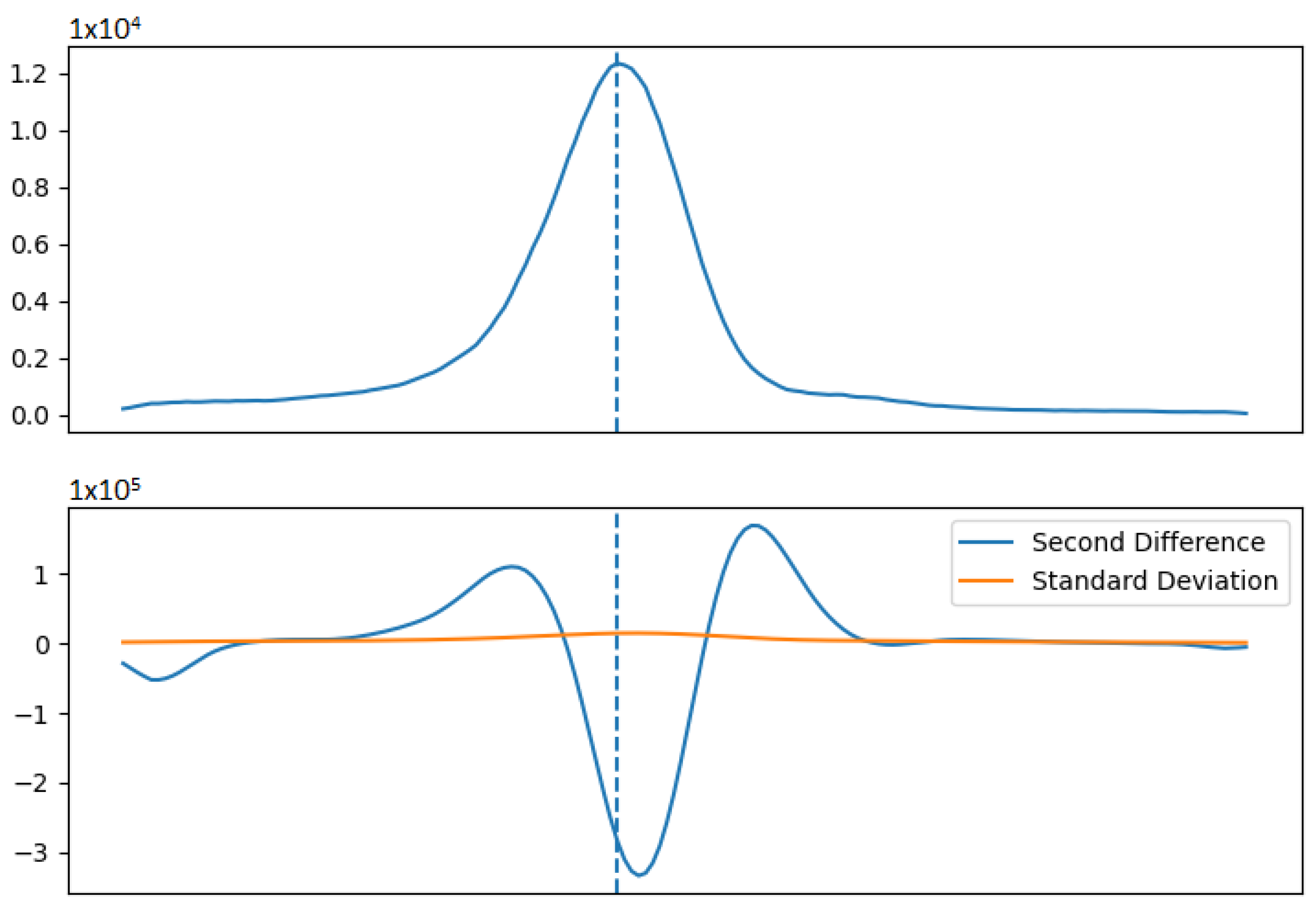
The first component of the code-base, the peak detection algorithm, is based on Mariscotti’s second difference method [8]. This method continues to be heavily utilised in computer systems performing peak searches, especially in spectroscopy software such as Genie™ 2000 [15]. It is centred on the underlying principle that for a Gaussian peak on a linear background, the second derivative will only be non-zero in the presence of curvature, such as a peak. This is demonstrated schematically in Figure 2, as the ’second difference’ plot of the upper peak.

The ‘second difference’ is the discrete analogue of the second derivative and is given by:

$$S_i=N_{i-1}-2N_i+N_{i+1}$$

(1)

where $N_i$ is the count in the ith channel. The standard deviation, $F_i$, of this derivative analogue is given by:

$$F_i=\sqrt{N_{i-1}+4N_i+N_{i+1}}$$

(2)

These are calculated for all i and smoothed multiple times by summing neighbouring values:

$${\tilde{S}}_i(z,w)=\sum _{j_1=i-m}^{i+m}···\sum _{j_z=j_{z-1}-m}^{j_{z-1}+m}{S}_{j_z}$$

(3)

where ${\tilde{S}}_i(z,w)$ is the smoothed second difference, z is the number of sums completed and $w=2m+1$. The optimum values for z and w found empirically by Mariscotti are 5 and $0.6\mathrm{\Gamma }$ respectively [8], where $\mathrm{\Gamma }$ is the full width at half maximum (FWHM) for peaks in the spectrum (a value, defined by the Gaussian distribution, that is specific for a given detector material, yet consistent across all peaks-referenced as a percentage value at the 662 keV Cs–137 photopeak). This smoothing procedure works well for single peaks which are well resolved spatially. However in the case of multiple peaks very close together, the result of this smoothing may be a single broad peak. Relative intensity comparisons already included in the identification algorithm may help to resolve this issue, however there is no alternative smoothing procedure currently implemented for cases such as this.

Smoothing is necessary to reduce the standard deviation relative to the second derivative and remove high-frequency noise from the spectral data that would otherwise result in the false identification of small peaks associated with such non-peak ‘ripples’. Peaks can therefore be identified with the condition $\mid S_i\mid >f{F}_i$, where f is the factor of confidence. They can also be resolved from some types of non-linear background using this condition since, in some cases, the second difference will be much larger in the presence of a peak than for curved background features. Here, through empirical analysis and refinements, a value of $f=3.5$ was chosen to detect peaks for ‘static’ (pre-recorded/post-processed) spectra read into the software [5]. For ‘dynamic’ (online) spectra, fluctuations as a result of the source-detector environment may necessitate a smaller confidence factor. Once a peak(s) is identified within a gamma-ray spectrum, its energy and intensity are appended to various arrays so an attempt can be made to identify the contributing isotopes by their comparison with a database of known gamma emitters.

Through the use of a configuration file within the module, it is possible to change various parameters affecting the peak search. This file allows the discriminators to be changed so that the peak search only takes place in a specific range of energy of the spectrum (e.g., between 300 keV and 2250 keV). The channel-energy relation parameters (slope and y-intercept of the line or coefficients of the polynomial if required) are found within this configuration file and can easily be changed to fit the spectrum/detector being used. A FWHM estimate provided to the peak search algorithm is also found here, which can be changed to best match the spectrum being examined since this will affect the performance of the algorithm as detailed above. The value of f can also be varied in this file, which affects the sensitivity of the algorithm to parts of the spectrum with negative second derivative. Essentially, this value represents the limit of detection (LoD) for the method. Also contained in the configuration file are: a list of common isotopes to be parsed when attributing an isotope to a peak if other identification methods within the module are otherwise unable to do so (detailed in the next section); a setting for the isotope library being used and the detector material and thickness which are used to select the energy-efficiency relation (exponential function) if one is present in another separate file for the same material/thickness.

2.2. Peak Fitting

Once a peak has been found, a Gaussian fit is calculated for it along with a goodness of fit statistic. Firstly, a background subtraction is applied to the peaks in the raw spectrum. This is done by taking the average of the 10 channels immediately before the peak and the 10 channels immediately after it. A straight line is calculated based on these values and numbers corresponding to the points on this line are taken away from the channels in the peak.

In order to fit the peak, the ‘curve_fit’ function from SciPy’s ‘optimize’ package in python is utilised [16]. The function is given the data to fit and the fit function as well as initial guesses for the parameters in the fit function. The ‘curve_fit’ function then cycles through parameters in an attempt to find the optimum fit. The optimum Gaussian parameters can then be used for the isotopic identification including the central value corresponding to the peak energy. The goodness of fit is tested using an extension of the coefficient of determination: the adjusted $R^2$ or ${\overline{R}}^2$ value. This provides an indication of how closely the fit matches the actual spectrum. The value of ${\overline{R}}^2$ used here was proposed by Ezekiel and is given by:

$${\overline{R}}^2=1-(1-R^2)\frac{n-1}{n-p-1}$$

(4)

where $R^2$ is the coefficient of determination, p is the total number of variables in the model and n is the sample size [17]. The adjusted $R^2$ was chosen for this method since it is not improved simply by adding more points; and so provides a more accurate measure of the goodness of fit.

2.3. Isotopic Identification

To determine the isotope(s) responsible for the peak(s) identified following the application of the formerly described second derivative method, a number of conditions, scenarios and characteristics must be assessed and implemented. Analogous to the multiple point recognition that underpins highly accurate human fingerprint identification; a similar multiple ‘feature’ (signature) approach is also employed as part of the peak screening, identification and discrimination methodology where multiple peaks are identified within a spectrum. Herein, the candidate isotope(s) attributable to each photopeak are cross-checked against/compared with all other second derivative identified peaks within the spectrum for common radionuclide identifications at different energies; utilising the primary, secondary and/or any number of potentially multiple gamma-ray peaks derived from the isotope. Detecting such multiple emission peaks associated with a single isotopic species (e.g., Bi-214 and Pb-214) makes identification through their characteristic ‘spectral fingerprint’ markedly easier, alongside reducing the peak ascribing error and uncertainty—as the likelihood of other emitter(s) yielding photopeaks with multiple, similar, gamma energies is unlikely; albeit with a number of caveats and considerations.

While more applicable to scenarios associated with the identification of a mono-energetic gamma emitter in contrast to multiple-peak ‘fingerprinting’ of isotopes with two (or more) characteristic emissions (thereby allowing for such an internal ‘validation’ and confirmatory ‘cross-checking’ of the other peaks existence), if the algorithms isotopic identification is incorrect, this would consequently indicate the presence of another (fortuitous) source (or sources), emitting at similar energies. This could also result from one or a combination of; (i) local attenuating materials around the source serving to introduce minor modifications the peak energy—consequently downwards ‘shifting’ the peak position from the ‘true’ value [18], and/or (ii) variations in the detectors intrinsic (energy and geometry dependant) photon absorption efficiency inducing minor peak shifts [19]. Therefore, within this embeddable python module developed for integration into various software platforms (primarily those utilised for robotic deployments and inspections, such as the ROS) multiple emitters are ascribed to a photopeak in scenarios where their energies are comparable and cannot be differentiated (a discussion of this, the error/uncertainty propagation and the algorithms transcription of the peak ID(s) within the python module are subsequently detailed below). It is noted that this contribution from the ‘environment’ in which the radioactive source resides represents a significant and complex contribution to the (various detector types) intrinsic detection efficiency across the full energy range of incident gammas [18].

While the applicable Mass Attenuation Coefficients, $\mu /\rho$ (and the associated Mass Energy-Absorption Coefficients, $\mu en/\rho$) are empirically and mathematically well constrained by organisations such as the US National Institute of Standards and Technology (NIST) [18] for various elements, mixtures, compounds and tissue types across the broad gamma ray photon spectrum; this is not true for more complex systems. Here, the inhomogeneity and contextual variability associated with sources contained within ‘real-world’ field/site decommissioning and assay scenarios envisaged for the deployment of this module introduces considerable complexity due to the resultant variations in photopeak intensity (at different energies). Whereas the detection efficiency and associated relative peak intensities for multiple photopeak emitting radionuclides are well-calibrated (for both detectors and geometric configurations) when associated with laboratory scenarios—delivering minimal uncertainties and errors for peak-fitting when using known inter-peak magnitudes, such an adoption of this approach is not possible, nor reliable, in this instance due to variations induced through the source-detector configuration. Therefore, the relative intensities of a radionuclides multiple photopeaks are not used as the primary discriminator/identifier of an isotopes occurrence—with reference peak intensities rather only used (alongside large tolerance values) to corroborate peak determination.

As detailed formerly, resulting from the Gaussian nature of photopeaks, such a mathematical fit can be easily applied to a single peak, unless it is comprised of more than one contribution. In this scenario, the peaks are ’subdivided’ with additional source(s), from the radionuclide lookup tables, ascribed as a contribution to the peak; identified as being erroneously large/non-Gaussian in order to make the peak area consistent relative to other peaks. Dealing with such peaks that do not match the anticipated peak Gaussian profiles through an alternate ‘division and contribution’ methodology is more challenging, and consequently no procedure currently exists for this.

As is the case for all solid-state type radiation detection materials, the inherent detection efficiency of such scintillators or semiconductors is greatest at the lowest incident gamma-ray energies (namely between 10 keV and 220 keV), although zero at energies tending to zero. Efficiency decreases rapidly (exponentially in many instances) as photon energies surpass 0.5 MeV [19]. If such detection efficiencies were to not depend upon the incident photon energy and assuming non-attenuated gamma rays, then the well-constrained relative peak intensities from non mono-energy gamma-emitting radionuclides could be easily normalised and compared, irrespective of the crystal material, to facilitate photopeak identification. However, as this is not the case—a correction function is required, based on this energy related decline in detection efficiency. As is conventional for most commercially available gamma detection systems [20], to compensate for, this python program includes an efficiency decay function, with parameters that are specific to each detector (such as; material, crystal thickness, shape and geometry)—which can be selected from pre-set values within the wrapper by specifying a material and geometry in the configuration file, or new parameters entered by the user. As this python code-base has been designed to operate on the readout derived from any USB-based detector module, all of these parameters are user-defined in the configuration setup and are based upon calibrations provided by the detector manufacturer or are mathematically/empirically derived, then added to the file containing the detection efficiency relations [19]. Where no efficiency calibration is able to be made, the program makes no attempt to subdivide peaks, as the relative intensities of peaks in this case are unlikely to be consistent with the expected spectrum.

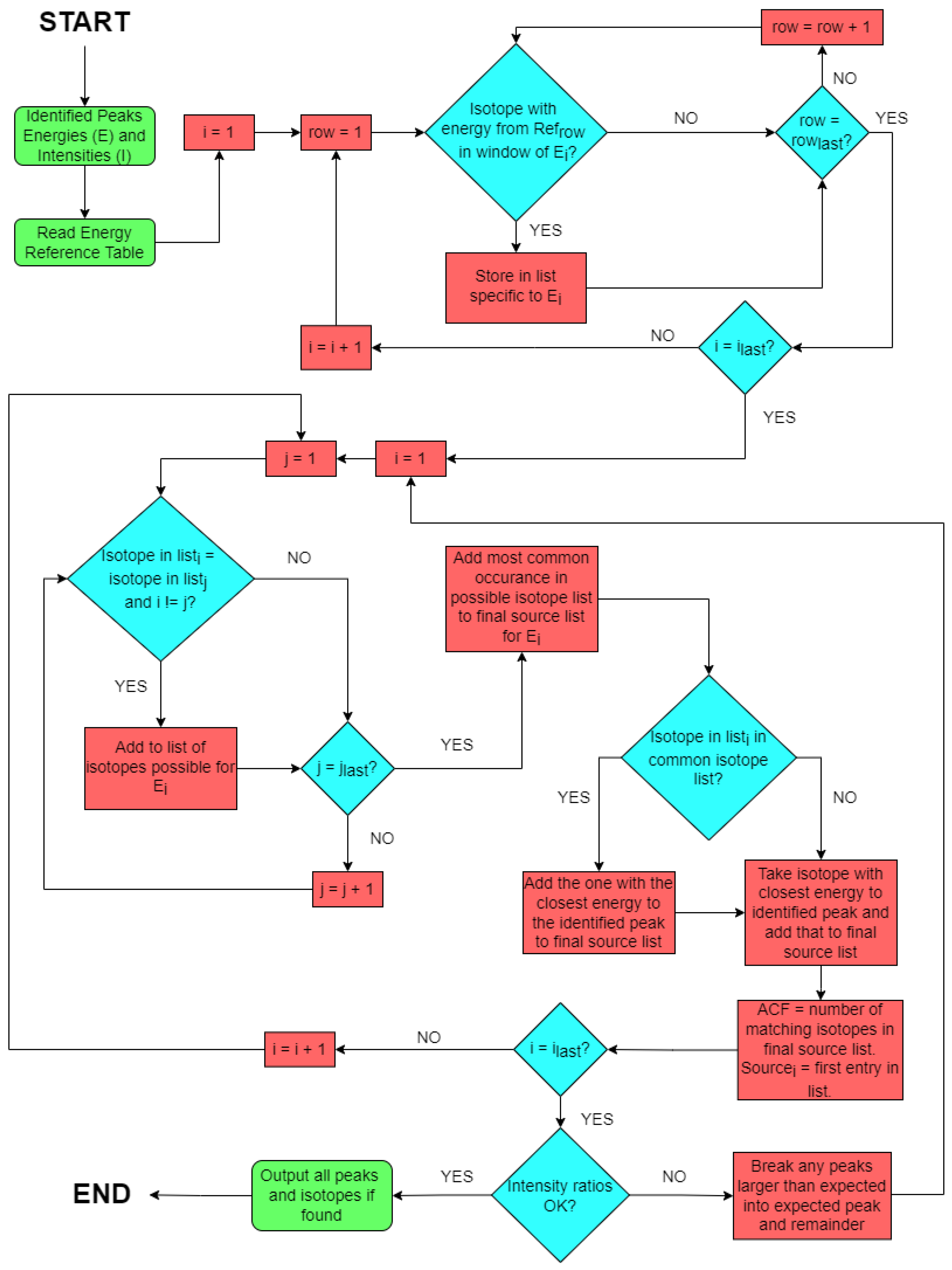
For scenarios where peaks are identified through the aforementioned ‘second derivative’ methodology and there are not multiple peaks with a common candidate isotope, a list of isotopes (with associated energies) known to be of common interest is cross-checked as part of a peak ‘pre-screen’. If a peak (or multiple peaks) energy is within a specified bin around that of an isotope in this list, then that isotope is assumed to be the incident radionuclide generating that peak—with the ID, intensity and error then output by the code-base. However, if no isotope(s) can be ascribed from the peak(s) present within this list, an attempt is then made to match the isotope(s) with a peak energy from the same (user) pre-selected reference list that most closely matches the energy of the peak. This deeper analysis consequently represents a more computationally intensive process.

As is typical for instances where only one photopeak is identified by the algorithm, e.g., Cs-137 (N.B. while the Cs-137 gamma spectrum is characterised by a primary emission peak resulting from the 0.512 MeV $\beta$⁻ decay, through the Ba-137m isomeric level, its disintegration to the same Ba-137 ground-state is also via a 1.17 MeV $\beta$⁻ emission—alongside accessory escape peaks), any reference to inter-peak intensity will be non-existent as no other emission photopeaks are present within the spectrum obtained. Therefore, where no other isotopic identification has been successfully made, peak energy is examined exclusively within the identification algorithm when attempting to correctly attribute an isotope to a peak. The algorithm simply attempts to attribute the source with the closest gamma energy to the identified peak.

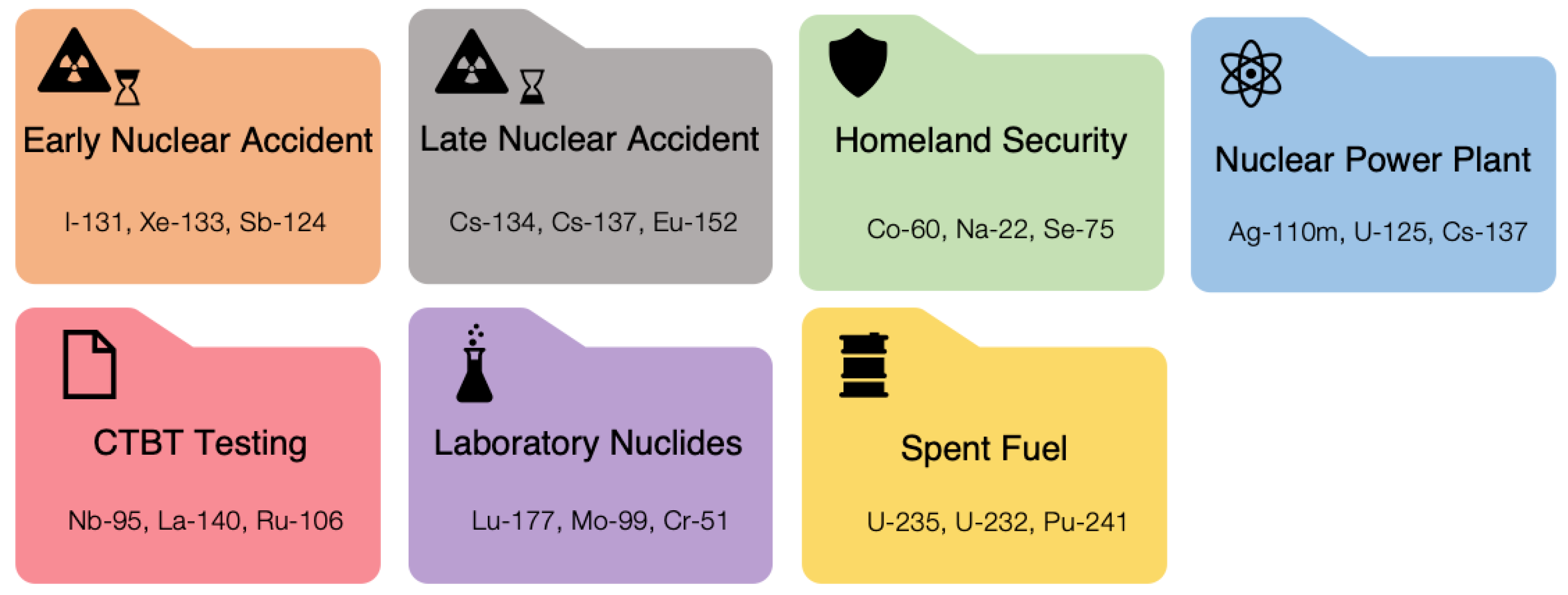
If the aforementioned initial ‘coarse’ peak ‘pre-screen’ identification fails to appropriately identify peaks based on the common interest suite of emitters (namely Cs-134, Cs-137, Co-60, Ag-110m, as well as those within the U and Th decay series) then a full search and fitting is performed. To facilitate a more accurate and efficient peak attribution from the algorithm by reducing the number of potential solutions, the contributing gamma-emitting isotopes are categorised into a number of libraries—a schematic representation of which is shown in Figure 3. During setup, the library most applicable to the scenario is selected by the user via the codes wrapper—although to avoid an incorrect ‘brute-force’ fitting if no peaks within the user-selected library are statistically appropriate, then the peaks contained in other libraries are searched for potential fits. This database is also included within the open-access code-base—with the details of the link to this repository contained within the information at the end of the manuscript. These seven libraries together comprise the scenarios for which gamma radiation would be encountered [21,22], and contain the isotopic information that is specific to each—albeit with a number of emitters common between groupings. For example, both I-131 and Xe-133 are specific to the ‘Early Nuclear Accident’ library (i.e., highly volatile radionuclides with short, days to week, half-lives that constitute the primary radioactive inventory following a reactor release event that are rapidly dispersed within the environment [23]), however, Cs-134 and Cs-137 are contained within both ‘Early’ and ‘Late Nuclear Accident’ suites (alongside being listed within other source libraries). While the ‘Early Nuclear Accident’ library comprised radioisotopes that are the primary inventory/dose contributor shortly after a reactor/site release, the ‘Late Nuclear Accident’ suite constitutes nuclides with longer (generally > 2 year) half-life that are not as volatile and short-lived. The species contained within the ‘Laboratory Nuclides’ comprise those used as part of biological tracing experiments or within medical procedures/treatments.

The three formerly outlined methods (same isotope to multiple peaks, isotope in list of common sources and closest energy) are all applied to each peak in order to obtain a candidate isotope. In order to give some idea of the robustness of the result found, an arbitrary confidence factor (ACF) has been defined and is returned with the table of isotopes output by the algorithm. This factor is an integer from 1 to 3 detailing how many of these methods agree on the obtained isotope. This factor is included as an extra check of the likelihood of a certain source being correct, though even if a value of 1 is obtained the result can still be correct.

If a peak is found and an isotope cannot be attributed to it using the methods included in the algorithm, the peak is reported without a value in the source column. A flowchart for the full isotope identification procedure, including the various caveats and sub-processes, is shown in Figure 4.

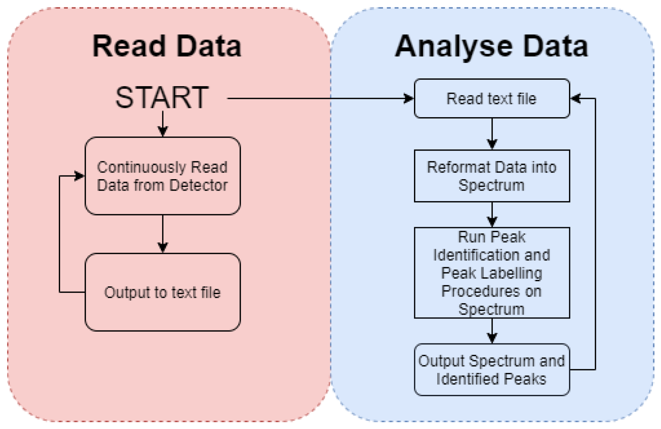
As formerly detailed, to facilitate the post-collection analysis of a gamma-ray spectrum alongside the online (live) isotopic evaluation vital for response and mapping scenarios, the algorithm’s wrapper script can be adapted. This user-configurable facility is such that it can handle both online ‘dynamic’ inputs (with the incoming detector channel data being appended to the array; serving to continually improve the counting statistics) as well as the post-processing of a ‘static’ output that comprises data (arrays) already written to a text file (or any other file format a user specified). The program can then parse either the formerly collected or online spectral data through the analysis code, where the peak(s) can be identified. These wrapper scripts allow changes to be made to the appearance of the output data and in the case of an online/dynamic input: the method of data collection and reformatting can be rewritten by the user to suit the system being deployed.

2.4. Detector and Algorithm Performance Trials

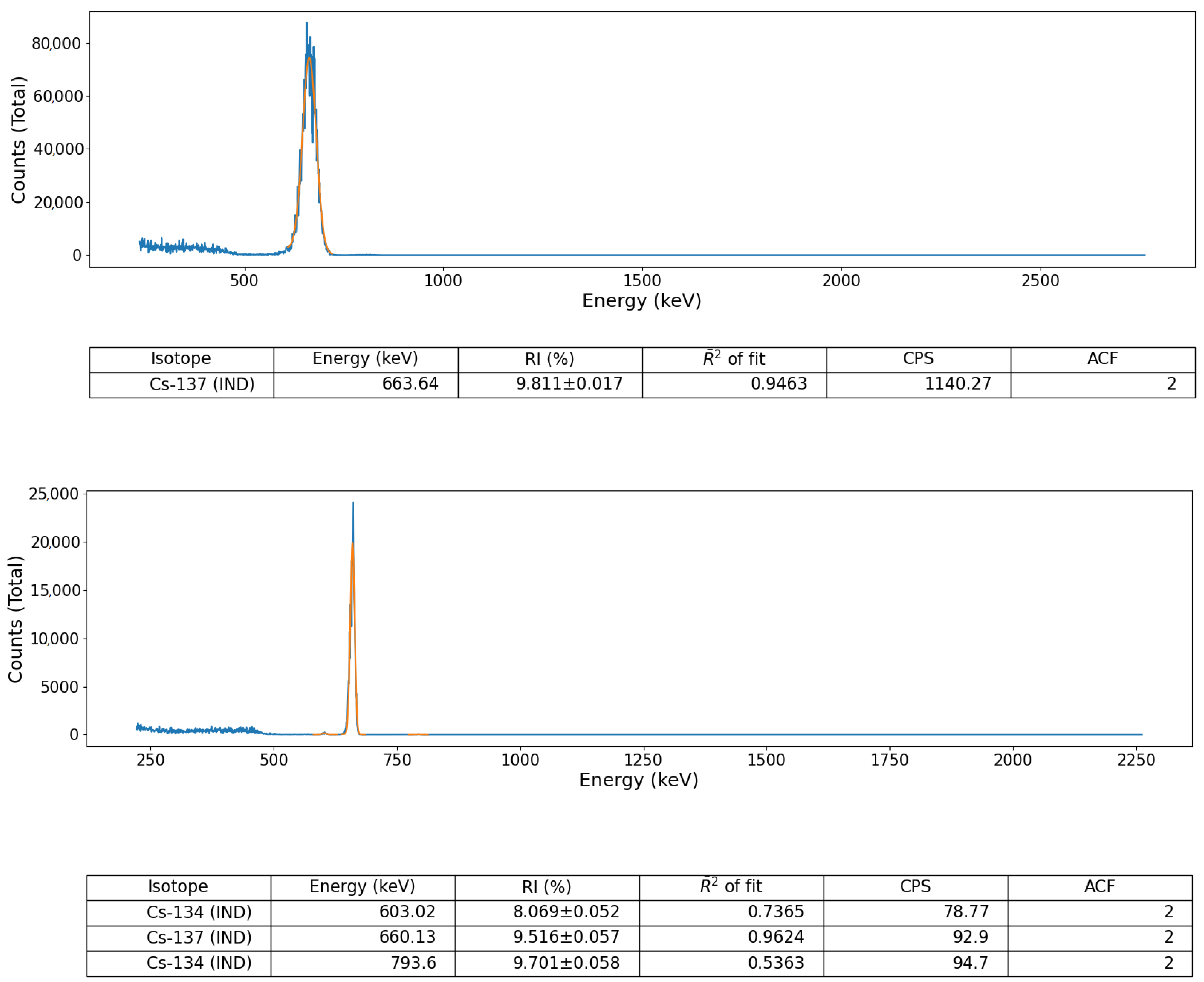
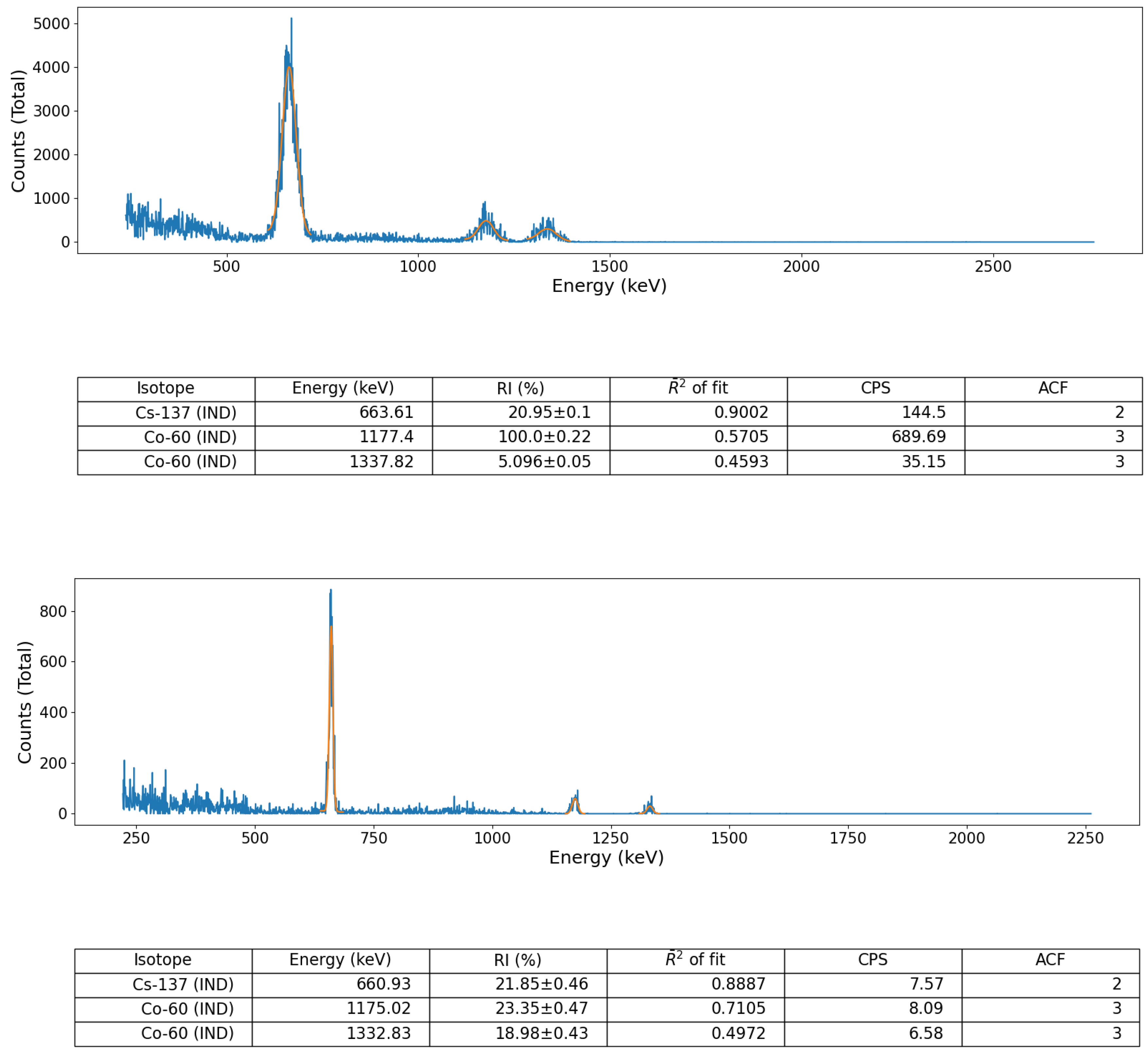
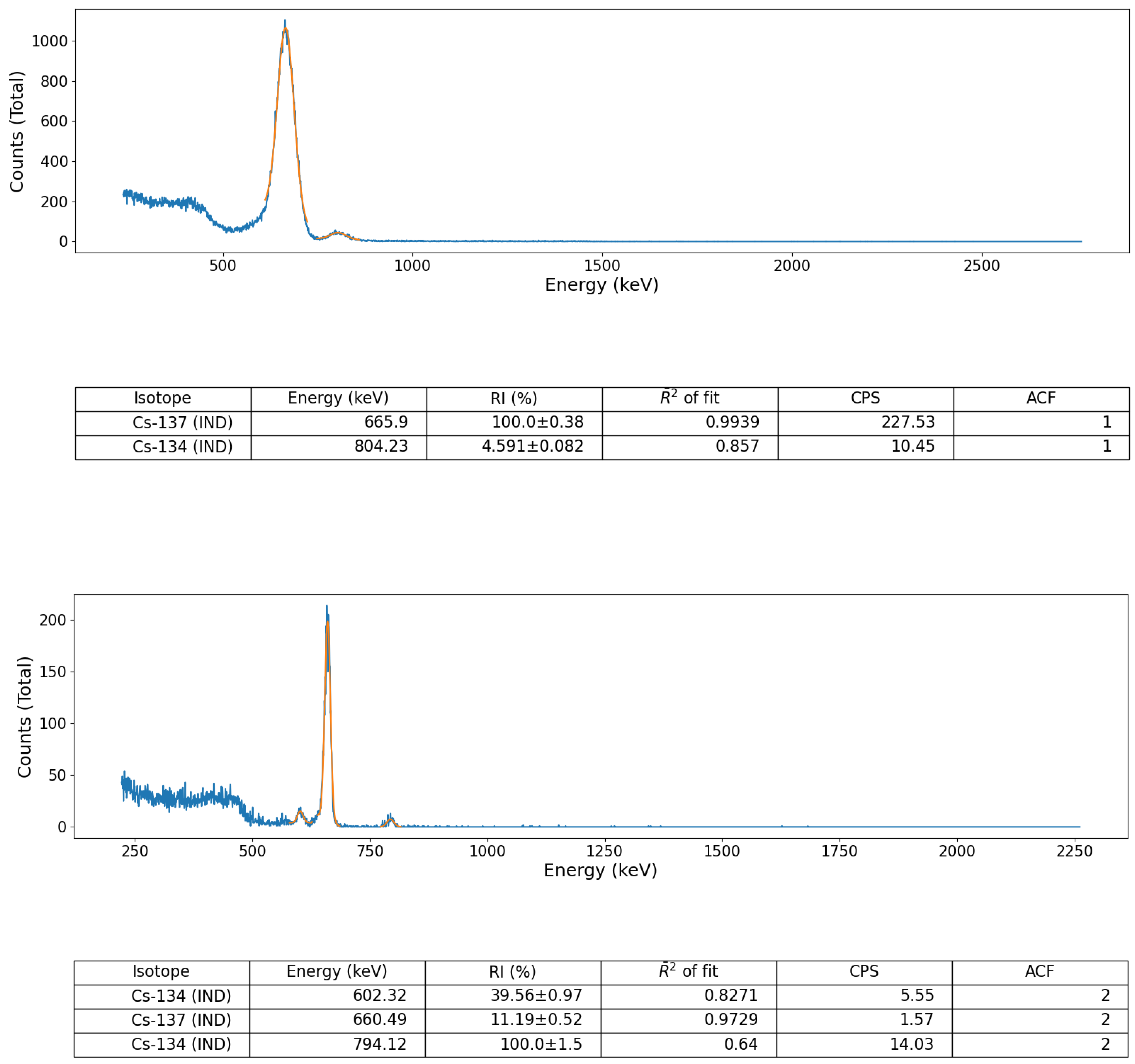
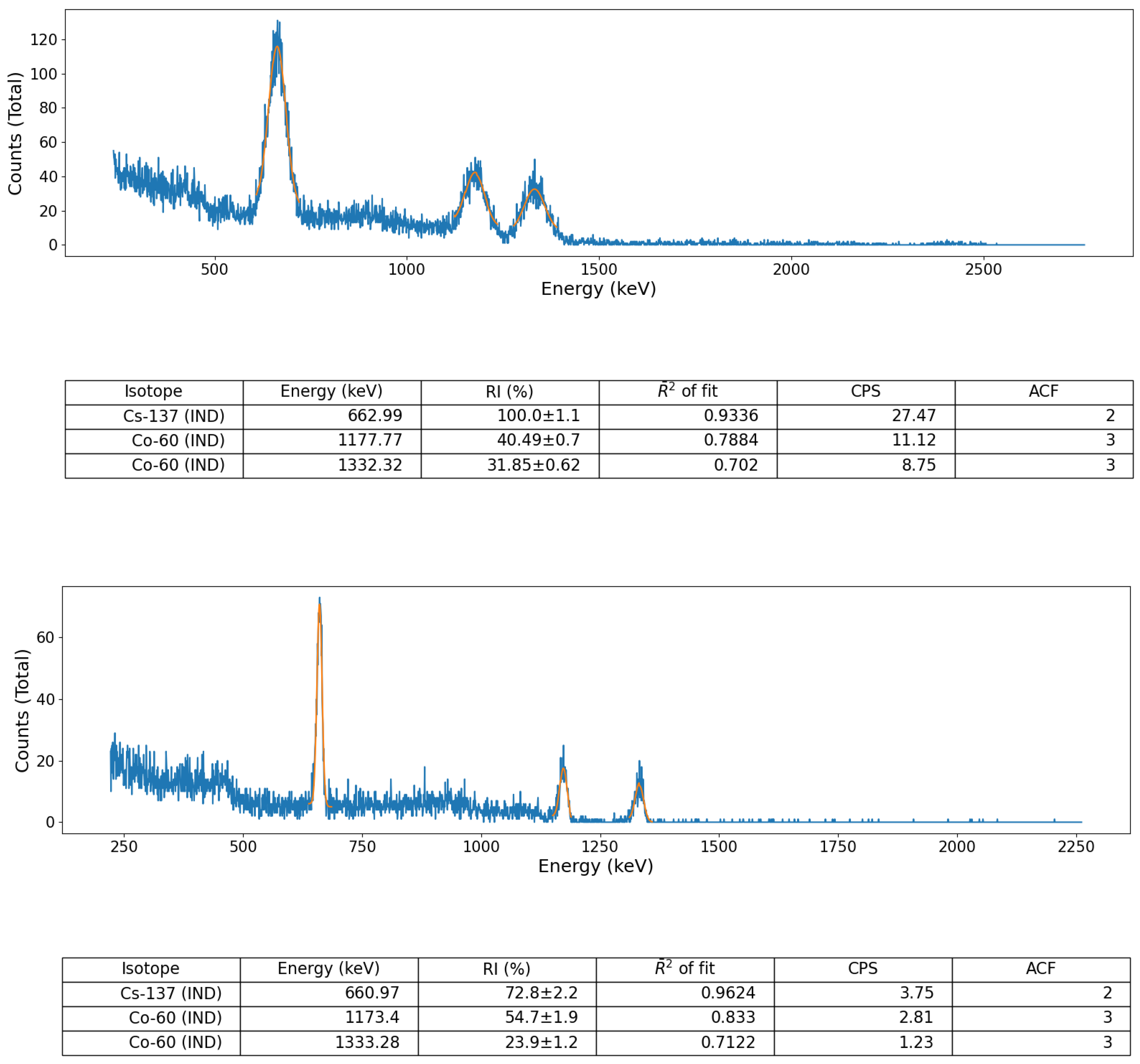
Validation of the peak identification algorithm was performed using a number of sealed radioactive sources (for both spectral file ‘post-processing’ and ‘online’, live, data-stream algorithm assessment) as well as on a suite of formerly collected spectra derived from a radioactively contaminated environment, detailed below. These sealed-sources, each with characteristic and well-defined gamma emission peaks, comprised; (i) soil derived from Fukushima Prefecture (Japan) radioactively contaminated with Cs-137 and (ii) a multi-radionuclide gamma-ray calibration coupon (QCRB22618 from Eckert and Ziegler™), constituting emitters (with activities at the time of production in 2016) detailed in

Table 1. Radioactive emitters and activities (at the materials time of production in 2016) contained within the Eckert and Ziegler™ multi-radionuclide calibration source. The isotopes successfully identified by the peak identification program during testing (detailed in Section 3) are in bold.

Isotope	Gamma Energy (keV)	Activity (Bq)
Pb-210	47	$4.02\times {10}^4$
Am-241	60	$3.43\times {10}^3$
Cd-109	88	$1.60\times {10}^4$
Co-57	122	$5.77\times {10}^2$
Ce-139	166	$6.91\times {10}^2$
Hg-203	279	$1.51\times {10}^3$
Sn-113	392	$2.46\times {10}^3$
Sr-85	514	$2.83\times {10}^3$
Cs-137	662	$\mathbf{2}.\mathbf{75}\times {\mathbf{10}}^{\mathbf{3}}$
Y-88	898	$5.19\times {10}^3$
Co-60	1173	$\mathbf{3}.\mathbf{27}\times {\mathbf{10}}^{\mathbf{3}}$
Co-60	1333	$\mathbf{3}.\mathbf{27}\times {\mathbf{10}}^{\mathbf{3}}$
Y-88	1836	$5.19\times {10}^3$

.

For testing of the peak identification against online (live) data (compiled as a string of gamma-ray energies continually appended onto the end of a text file) spectra were derived of the aforementioned sources using; (i) a Kromek D3S combined gamma-ray/neutron spectrometer module (with gamma detecting CsI(Tl) crystal of 51.0 mm × 25.4 mm × 12.5 mm dimensions, a and LiF:ZnS neutron detecting crystal of 32 mm × 100 mm dimensions) [24], (ii) a Hamamatsu C12137-01 CsI(Tl) spectrometer module (of 38.0 mm × 38.0 mm × 25.0 mm crystal dimensions) [25], and (iii) a Kromek GR1 CdZnTe (CZT) semiconductor micro-gamma spectrometer (of 10 mm × 10 mm × 10 mm crystal dimensions) [26]—with the serial output strings from each parsed through the peak identification code-base. In each instance, the applicable radionuclide library (‘Nuclear Power Plant’ for both sources) was selected in the codes associated wrapper function—alongside the detector-specific parameters (such as; crystal type, size and geometry). It is noted that while more advanced, higher-sensitivity and resolution radiation detector modules exist on the market, the highly miniaturised, rugged and USB-controlled solid-state units used in this work constitute those most widely employed within nuclear robotics, in-field/site characterisation/assay and decommissioning. Their low-cost and accessible (unencrypted) output format additionally allows for ready integration of such devices into a wide range of monitoring applications not possible for larger, albeit potentially more sophisticated, detectors.

Tests on the algorithm were also performed using ’post-processed’ spectra obtained from the same calibration sources, again collected using the three aforementioned portable radiation detection systems commonly deployed for remote/robotic monitoring applications. The spectral data was parsed into the analysis code from a text file that comprised channel number vs. event frequency. It is noted, however, that the wrapper functionality within the code permits for other alternate data and file formats to be translated and parsed through the analysis code; such as .csv, .msc and, .spc.

The acquisition of spectral data (using the sealed-sources), for both online (live) and subsequent post-processing analysis via the algorithm was performed using a simple detector-source configuration in each instance. The experimental setup comprised the detector held within a conventional laboratory stand with the units crystal positioned such that its long-axis was directed vertically down, orthogonal to the bench—with the base of the detector (and crystal) at a height of 11 cm from the surface. Each 1 cm thick source was then positioned directly under the detector (resulting in a 10 cm separation), with spectra acquired for a duration of 5 min (real-time).

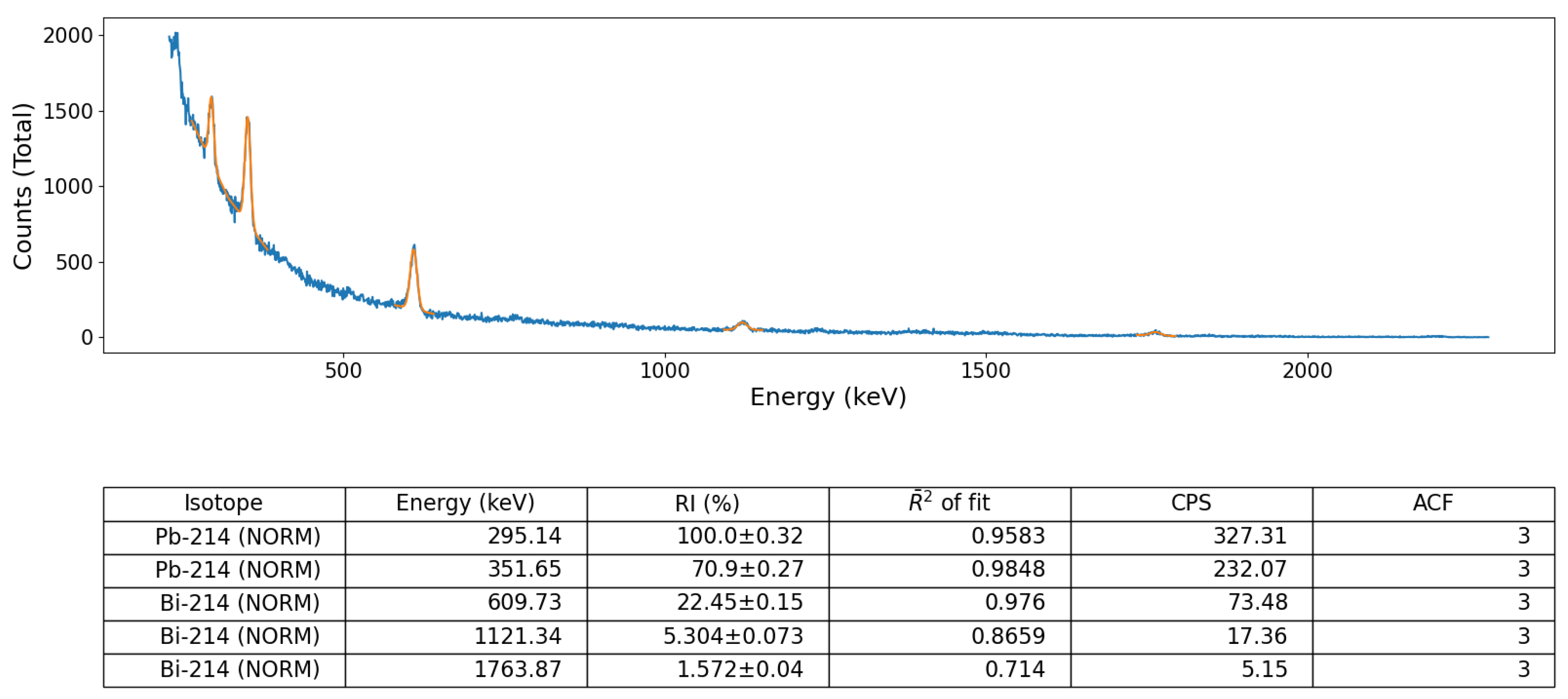
In addition, to provide a further test of the algorithm, away from the aforementioned well-calibrated/defined source-detector environment, a gamma-ray spectrum formerly obtained from the naturally occurring radioactive material (NORM) and Industrial (IND) associated radionuclide contaminated Pridneprovsky Chemical Plant (PChP) site in Dnieprodzerzhinsk, south Ukraine, was also used to validate the algorithm, owing to the multiple daughter radionuclide emission peaks associated with the U/Th decay chain (e.g., Bi-214, Bi-210, Pb-214, Pb-210). This measurement was obtained using the same Kromek GR1 CdZnTe detector module using the manufacturer’s KSpect™ spectral acquisition software, with the resulting spectrum stored (and exported) as a text file (of channel numbers vs. counts) for subsequent peak analysis using the python algorithm. An identical 5 min acquisition time was used to acquire the spectrum, with the measurement of the sample taken with the same 10 cm detector-sample separation.

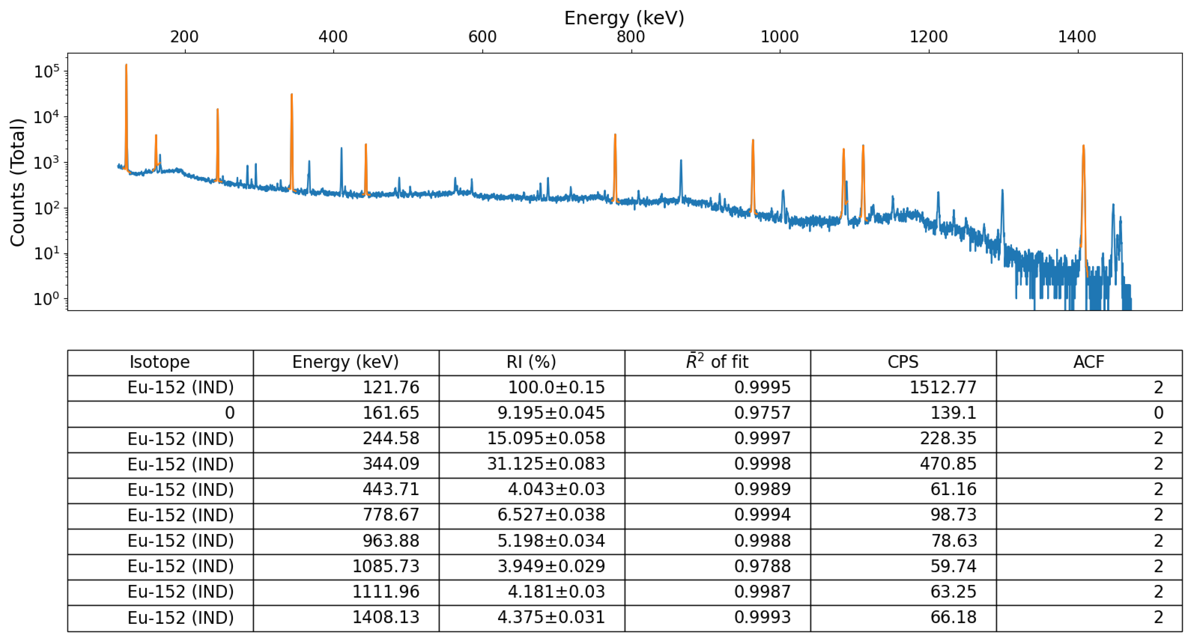
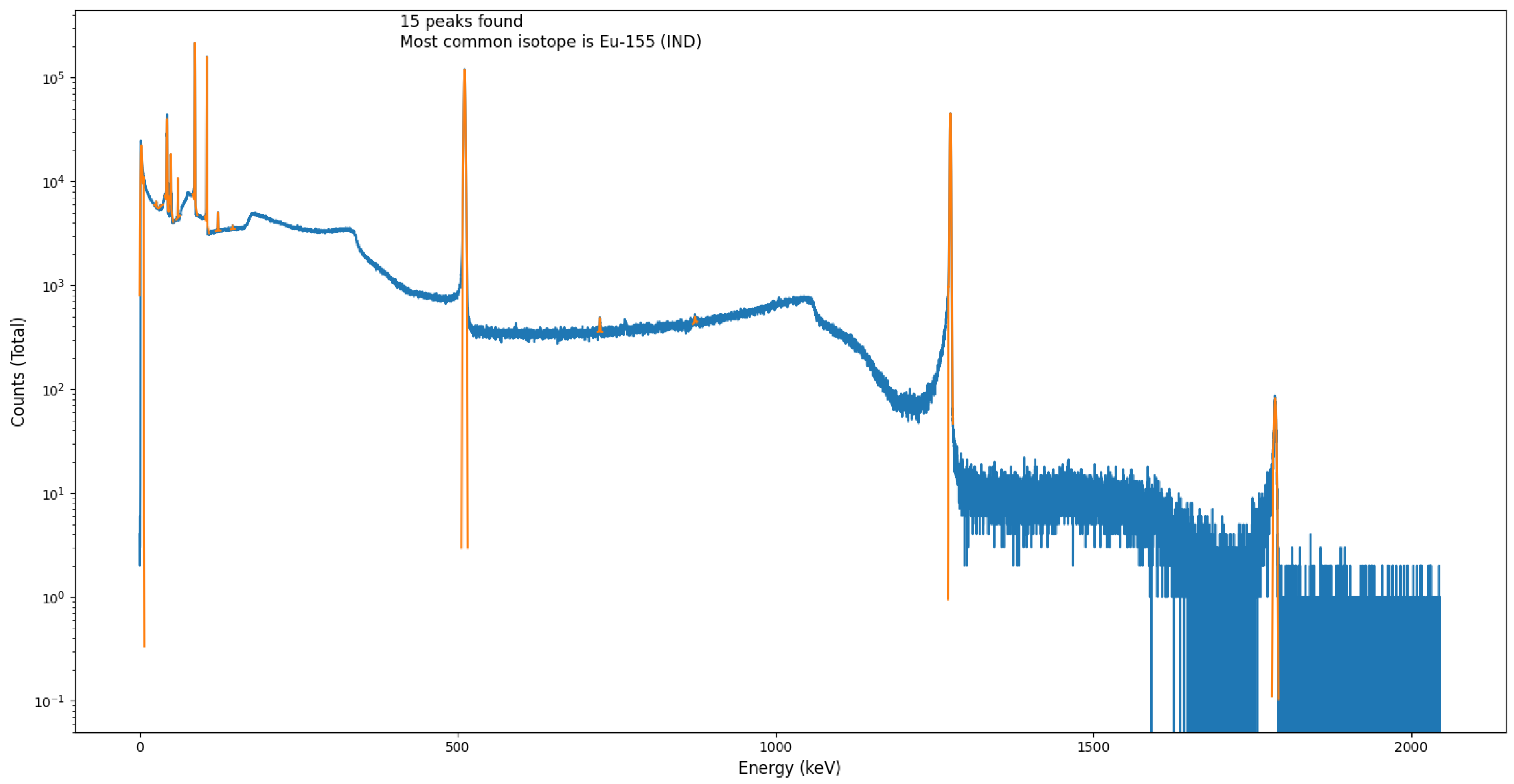
To numerically quantify the performance and accuracy of this python algorithm against other, accepted, peak-fitting approaches, the algorithm was additionally tested and quantified through the post-processing of a Eu-152 spectrum as well as the spectrum obtained from an Na-22 and Eu-155 source. A peak locate report was generated using Genie™ 2000 and compared to the peaks found using the module presented here for validation. The spectral data for these was obtained using the same experimental setup/methodology as detailed above; using a Mirion Technologies (Canberra) SAGe™ Well detector [27]. While this detector possesses a superior FWHM value (of 2.2 keV at the 1332 keV Co-60 photopeak) than any of the other three radiation detector devices used for testing (of which the detector-specific FWHM value are inserted as parameters within the modules ‘wrapper’ code), the high cost, need for cooling, size and mass currently prevents this detector type being deployed by robotic or remotely operated systems—for which this code-base is developed to facilitate within such ROS applications.

3. Results

The gamma-ray spectrum derived from the exposure of the detector module to the NORM sample material at the PChP site is shown in Figure 5—comprising the various emission photopeaks across the (GR1) devices 30 keV to 3.0 MeV energy range. Also shown in Figure 5, as produced by the peak identification code, is the automatically generated results table. This plot shows that the contributing radionuclide peaks (from the uranium series) are correctly identified by the algorithm and ascribed an isotope and relative intensity (RI) value (calculated by summing the peak’s total counts using the original spectrum with the error arising from the Poisson uncertainty of the count), which is displayed alongside the peak energy, integrated counts per second (CPS), the adjusted $R^2$ value as an indication of goodness of fit and the ACF as detailed in Section 2.3. Resulting from the multiple emission peaks present within a NORM gamma-ray spectrum, the identification of such material is not a challenge for the algorithm as the ingrown isotopes (of Pb and Bi) all occur at discrete energies away from peaks characteristic of other radionuclides. The uncertainty in ascribing peaks is further reduced through the use of the integrated library function, where the potential source contributors are greatly limited through prior user-selection. A confidence factor (f) of 3.5 was used within the peak detection algorithm to obtain the results detailed in this section. As mentioned previously, this confidence factor also allows for the detection of peaks on the non-linear background shown in this plot. This is due to the second difference only exceeding its standard deviation scaled by f in the presence of the photopeaks, even for the curved edge background feature seen.

In contrast, the discrete single emission peak of Cs-137 represents a greater challenge for the materials radioisotope identification via this, as well as other algorithms—especially in online (live) where statistical/peak variations are introduced by data being continually appended into the array/text file. This is the result of the primary emission peak (at 662 keV) occurring close to those of Ag-111m (657 keV and 677 keV) causing uncertainty in the peak energy determination; especially when the contributing source is of low activity, at distance from the detector, or impacted by any shielding/attenuating interference(s). However, following the selection of the ‘Early Nuclear Accident’ or ‘Late Nuclear Accident’ radionuclide libraries within the peak identification algorithms wrapper code, as shown in Figure 6, the code-base is able to identify the Cs-137 contribution more often than if the full catalogue of isotopes were available for selection. As Cs-134 and Cs-137 (as well as other volatile and more short-lived radionuclides) are the primary radionuclides arising from an accidental nuclear facility release [21,28] (e.g., reactor loss of coolant incidents, reactor/fuel integrity losses as well as gaseous discharges from reprocessing sites) such as Chernobyl and Fukushima, before then residing in the environment for decades to follow as a result of their high fission product yield and longer half-lives, the radionuclides accurate identification is essential for both initial and long-term monitoring. To support such isotopic assay—both on-site and in the local/global environment, it is illustrated that this algorithm is able to perform online identification of the Cs-137 containing source material using both the Kromek GR1 and Hamamatsu C12137-01 detectors; the results of which are shown in Figure 6.

Alongside the online (live) peak identification of the Cs-137 sealed source, Figure 7 shows the corresponding online spectral analysis of the Eckert and Ziegler™ multi- radionuclide gamma-ray calibration coupon (the emitters within this coupon are outlined in Table 1), from which the python module was able to identify the significant Cs-137 and Co-60 photopeaks—both with high levels of statistical confidence. The absence of the Y-88 emission and other listed sources and energies from the gamma-ray spectra of the calibration standard, principally results from a combination of two factors; (i) the age of the source; with most isotopes possessing a half-life of less than a year, the activity of the radioisotope within the reference standard is now much less than the original activity of the source and less than that of Co-60—which itself has a half-life of circa thirty years. In addition to (ii) whereby for all gamma-ray spectrometers, the energy efficiency of the device is markedly reduced at these higher gamma energies (in contrast to the lower, e.g., sub 800 keV photo peaks), therefore while the activity may be equitable or even greater, the magnitude of the peaks within this portion of the spectrum are considerably reduced in contrast to those at lower gamma-ray energies.

As well as the online (live) peak identification of spectral results parsed through the code-base as a continual string/array from the detectors serial USB output (appended to the base of a continually updated .txt file), the algorithm is additionally able to undertake radioisotope identification (post-processing) of static/formerly collected spectral datasets. The results of this ‘once through’ peak identification for the same multi-radionuclide calibration and Cs-137 sources are shown in Figure 8 and Figure 9, respectively. As for the online (live) spectral analysis, the program is able to accurately identify peaks and ascribe the appropriate gamma emission source. The uncertainties associated to the (normalised) integrated peak areas (RI) are a result of the Poisson uncertainty associated with counting, which is larger for smaller and thinner peaks. Examples of this can be seen in Figure 7.

The 662 keV peak is identified for Cs-137 in the spectra gathered for the contaminated soil (Figure 6 and Figure 8). Overall, the peak search and fitting performed as expected, yielding good estimates for the values in the table based on the user specified parameters.

As seen in Figure 8, the program can detect and attribute minor photopeaks (e.g., Cs-134—occurring as a trace residue within the Cs-137 sealed-source) where the signal fluctuation is above the background and yields a high second derivative value. These effects can be limited through further refinement of parameters; specifically the adoption of higher confidence factors or higher threshold values would help eliminate these identifications. However, modifying these values may conversely lead to a lower probability of detecting peaks which are present within the spectra. While this suppression may be advantageous in certain circumstances, the identification and attribution of such peaks is the primary function of an embeddable python peak detection system—where the ultimate interpretation, acceptance or refutation of the software’s results, is performed by the user.

To additionally evaluate this peak-fitting methodology, the spectrum of a Eu-152 source, the spectrum of which had been recorded using a SAGe™ Well detector [27], was analysed by the module, using the “laboratory miscellaneous” isotope library. The result of post-processing this spectrum file through the algorithm is shown in Figure 10. The program was able to identify many of the emission peaks present and attribute the correct source. The thresholds here were set so that only peaks with heights above 0.5% of the maximum bin count recorded were identified. A confidence factor of $f=5$ was also chosen for this test. As can be seen, there is one peak that was discovered which could not be assigned an isotope at 161.65 keV. This is because in the library used, there are no listed peaks close to this energy. However, no photopeaks outside of those within the Eu-152 system were identified by the algorithm. The peaks show very small RI uncertainties within the Eu-152 peak identified spectrum. This is due to their high number of counts. The peak search was able to identify 10 peaks characteristic of the Eu-152 decay scheme with good energy resolution. The module performed as expected and with further refinement of the user specified values, such as an energy-efficiency relation, even more peaks may be identified and less errors may be observed.

Finally, in order to validate the performance and parameters found by the peak-fitting program, the spectrum of an Eu-155 and Na-22 mixed source, recorded using a well detector as described for the Eu-152 source, was analysed. The spectrum, which can be seen in Figure 11 was first run through Genie™ 2000 and a peak locate report was generated. This same spectrum was then run through the module outlined in this work. For both, a confidence factor, $f=3$ was used. As before, the module was able to correctly identify the isotopes responsible for the spectrum, finding and labelling 2 Na-22 peaks and 6 Eu-155 peaks correctly. A further 3 peaks were attributed to Eu-154 and the others to parent isotopes of Eu-155 (Pu-241 and Np-237). Only 2 were not able to be identified. The full peak report results for both Genie™ 2000 and the python module are outlined in

Table 2. Peak reports for a Eu-155 and Na-22 mixed source spectrum recorded using a SAGe well detector with 5 min acquisition time. Results are reported from Genie™ 2000 and the module outlined in this work. Spectrum can be seen in Figure 11.

Genie™ 2000				Python Module				Error Between Genie™ and Python Module Values (%)
Peak Energy (keV)	FWHM (keV)	Net Peak Area	Net Area Uncert.	Peak Energy (keV)	FWHM (keV)	Net Peak Area	Net Area Uncert.	Peak Energy	FWHM	Net Peak Area	Net Area Uncert.
1.68	0.64	89,490	602.95	2.44	2.38	348,003	1949.69	45.24	271.88	288.87	223.36
26.53	0.58	2827	471.26	26.48	0.58	3404	340.62	0.19	0.00	20.41	27.72
33.18	0.58	3758	460.35	33.11	0.43	416	1244.29	0.21	25.86	88.93	170.29
38.90	0.20	1715	642.04	-	-	-	-	-	-	-	-
42.79	0.98	273,100	580.42	42.79	1.08	57,532	447.24	0.00	10.20	78.93	22.95
45.33	0.98	24,660	296.09	-	-	-	-	-	-	-	-
48.66	0.62	71,840	348.92	48.69	0.58	30,398	338.04	0.06	6.45	57.69	3.12
49.99	0.62	19,430	239.71	-	-	-	-	-	-	-	-
58.03	0.58	1355	189.17	-	-	-	-	-	-	-	-
60.01	0.59	31,870	285.92	59.94	0.62	12,573	644.53	0.12	5.08	60.55	125.42
65.02	0.15	591	578.02	-	-	-	-	-	-	-	-
75.06	1.03	5593	308.17	-	-	-	-	-	-	-	-
76.56	1.04	4942	315.38	-	-	-	-	-	-	-	-
86.55	0.64	1,154,000	1282.50	86.51	0.65	1,110,633	1113.84	0.05	1.56	3.76	13.15
95.53	0.43	736	412.29	-	-	-	-	-	-	-	-
105.31	0.66	873,500	1075.27	105.30	0.70	875,114	982.41	0.01	6.06	0.18	8.64
123.08	0.64	8803	418.77	123.08	0.73	10,022	293.82	0.00	14.06	13.85	29.84
146.09	0.74	1734	450.48	146.05	0.99	2,472	447.69	0.03	33.78	42.56	0.62
247.93	0.94	724	212.20	-	-	-	-	-	-	-	-
252.68	0.95	1569	233.89	-	-	-	-	-	-	-	-
398.07	0.36	−33	182.93	-	-	-	-	-	-	-	-
511.14	2.45	2,366,000	1727.85	511.05	2.53	2,441,198	1620.06	0.02	3.27	3.18	6.24
592.13	0.24	345	144.71	-	-	-	-	-	-	-	-
662.76	0.28	−6	113.62	-	-	-	-	-	-	-	-
723.58	1.11	1255	162.06	723.47	1.13	1208	126.52	0.02	1.80	3.75	21.93
756.90	1.42	410	88.04	-	-	-	-	-	-	-	-
763.17	1.42	597	95.67	-	-	-	-	-	-	-	-
851.30	0.37	114	142.06	-	-	-	-	-	-	-	-
873.56	0.32	1015	202.98	873.33	1.59	907	290.26	0.03	396.88	10.64	42.99
996.51	0.30	533	172.53	-	-	-	-	-	-	-	-
1005.15	0.78	1171	239.78	-	-	-	-	-	-	-	-
1275.05	1.78	688,500	866.71	1274.85	1.84	678,525	841.41	0.02	3.37	1.45	2.92
-	-	-	-	1785.82	3.27	1843	60.03	-	-	-	-

.

For all peaks except the initial ‘rising edge’, the percentage error on the centroid energy calculated by Genie™ 2000 versus the python module described here was equal to or less than $0.21\%$, this suggests the 2 modules are in good agreement over peak locations. Similarly, most of the FWHM values agree with less than 30% error. In cases where this is not true, this can also account for the discrepancy between the peak areas and their uncertainty. Some work on area calculation is required, this functionality will be improved in the future versions of the module in the hopes of decreasing the errors.

4. Discussion

The python module developed, as well as the underpinning methodology and results of its laboratory and preliminary validation are detailed in this work; showing promising performance when faced with both simple, site specific spectra with a single photopeak (Cs-137) as well as more complex spectra found in laboratories (Eu-152). The ${\overline{R}}^2$ values validate the peak fitting in most cases and provide reassurance that the peaks are Gaussian in nature. Overall, the method performs well and is often able to identify peaks with high energy resolution and in most cases correctly identify isotopes responsible if an isotope library is selected.

This system represents a powerful yet efficient tool for use in a suite of embedded radiation detection and identification applications-such as those where deployments (and monitoring) are performed using highly portable detectors transported by platforms controlled by the ROS. One such factor is that with minimal effort, the code-base can be adjusted for a wide range of detector types, geometries, crystal compositions and output formats—therefore not restricting it (or ’locking’ it in) to a single detector type, scintillator material or, more crucially, manufacturer; as the range of available detectors (from an increasing number of manufacturers) further grows. This multi-layer approach means that through the use of different intuitive wrapper scripts, different input methods and detectors can be readily integrated/upgraded to work with the primary peak identification code-base. Owing to the modular nature of the code-base, it is very easy to edit the data output from a detector to be in the output format that the down-stream peak identification program(s) expect and can subsequently undertake the mathematical peak-fitting process, with results integrated into ’downstream’ components.

There are no processes which have a high complexity for CPU usage within the program. This means that peaks can be identified quickly once sufficient data is recorded for peak discrimination. This is advantageous for security/monitoring applications as possible threats can be screened and sorted swiftly. However, some optimization may be required, especially with the addition of more intelligent identification criteria or customised libraries of isotopes pertinent to specific deployment scenarios (e.g., NORM, radiological release event or power plant). While modern micro-controllers, such as the Raspberry Pi™ LattePanda™ and MicroPython™, are more than capable of solely undertaking this peak-fitting algorithm on their internal memory/CPU, a streamlined, computationally efficient and embeddable/parallel code-base is necessary owing to the simultaneous processes that are likely operating on the micro-controller. These functions include (semi-) autonomous navigation, simultaneous localization and mapping (SLAM), hazard avoidance, ‘safe’ route planning and swarm/multi-system mapping/investigation.

As is the case with any code-base, there exists plenty of scope of future refinement and capability enhancement. Future work will aim to include a number of improvements to the module such as the one detailed above. For example, it may be useful to include a graphical user interface (GUI) to improve ease of use for non-experts. Furthermore, extra functionalities such as the ability to have different confidence factors in different areas of the spectrum could be a useful improvement. This would reduce the uncertainty in peak finding in the noisy low energy part of a spectrum, without ignoring it entirely. The open source nature of this module means that it can be easily and collaboratively worked on into the future. This will ensure that the module has the functionalities required by its users and that it can be easily changed to fit specific needs.

There also exists the possibility of adding a process that complements the existing library functionality by producing additional ‘look-up’ libraries containing all of the peaks associated with a decay chain (e.g., U-238, U-238, Th-232). Therefore, if one (or multiple) characteristic peaks within a decay-series library were identified, the algorithm could also search for photopeaks associated with other radionuclides in that chain. While only serving to highlight more statistically probable matches, care must be taken to ensure that a ‘brute force’ matching does not occur, where the algorithm assumes that all of the decay chain is present (when it is not), or, that only peaks within that decay chain are available for fitting—with an ignorance of other photopeak contributors.

5. Conclusions

A python module has been successfully developed and implemented which performs rapid automated spectral analysis, removing the need for lengthy human involvement and post-processing. The module has the potential for use in robotically operated systems, controlled by non-experts, since the output is streamlined to include only the isotope(s) responsible for the identified photopeaks (alongside the associated fit and error analysis). The program works on both post-processed and online (live) input spectra, therefore possessing applications both in the lab and in situations where rapid real-time identification is a necessity. Possible applications include: site clean-up and decommissioning (with deployment through detectors and robotics systems) and security/monitoring of nuclear materials. The output can also be fed to other programs for further analysis. Any detector can be used (with a dedicated or modified wrapper) after changing only a few values in the configuration file, unlike other peak identification software which is often detector specific. As the fundamental detector-specific parameters are contained within the associated wrapped code-base, future work will seek to transition the detectors algorithm-derived output from the current peak/isotope windowed CPS value (which is highly detector specific and non-translatable between devices) to a more cross-detector applicable, widely utilised and meaningful value of activity (Bq/g).

References

1. Quigley, M. ROS: An open-source Robot Operating System. In Proceedings of the ICRA 2009, Kobe, Japan, 12–17 May 2009; Available online: https://www.researchgate.net/publication/233881999_ROS_an_open-source_Robot_Operating_System (accessed on 25 January 2021).
2. ORTEC® AMETEK Inc. GammaVision® 8.10, Gamma Spectroscopy Software. Available online: https://www.ortec-online.com/-/media/ametekortec/brochures/gammavision.pdf?dmc=1&la=en&revi\sion=8a3f8c8e-1157-44b3-b829-3641fd61da82 (accessed on 26 January 2021).
3. Mirion Technologies, (Canberra) Inc. Genie™ 2000 Interactive Peak Fit. Available online: https://www.mirion.com/products/genie-2000-interactive-peak-fit (accessed on 26 January 2021).
4. Fitzgerald, J.; FitzPeaks Gamma Analysis and Calibration Software. JF Computing Services. Available online: https://www.jimfitz.co.uk/fitzpeak.htm (accessed on 26 January 2021).
5. Yazid, P.I. Y-Spect: A Multi-Method Gamma Spectrometry Analysis Program. Atom Indones. 2013, 39, 40. [Google Scholar] [CrossRef] [Green Version]
6. Savitzky, A.; Golay, M.J.E. Smoothing and Differentiation of Data by Simplified Least Squares Procedures. Anal. Chem. 1964, 36, 1627–1639. [Google Scholar] [CrossRef]
7. Sterlinski, S. Analysis of digital data from a multichannel pulse height analyzer on gamma ray total absorption peaks in activation analysis. Anal. Chem. 1968, 40, 1995–1998. [Google Scholar] [CrossRef]
8. Mariscotti, M. A method for automatic identification of peaks in the presence of background and its application to spectrum analysis. Nucl. Instrum. Methods 1967, 50, 309–320. [Google Scholar] [CrossRef]
9. Garner, S. Peak Doctor v 1.0.0 Labview Version, Version 00. 2014. Available online: https://www.osti.gov/biblio/1311399 (accessed on 25 January 2021).
10. Jarman, K.D.; Runkle, R.C.; Anderson, K.K.; Pfund, D.M. A comparison of simple algorithms for gamma-ray spectrometers in radioactive source search applications. Appl. Radiat. Isot. 2008, 66, 362–371. [Google Scholar] [CrossRef] [PubMed]
11. Ely, J.; Kouzes, R.; Schweppe, J.; Siciliano, E.; Strachan, D.; Weier, D. The use of energy windowing to discriminate SNM from NORM in radiation portal monitors. Nucl. Instrum. Methods Phys. Res. Sect. A 2006, 560, 373–387. [Google Scholar] [CrossRef]
12. Sullivan, C.J.; Garner, S.E.; Butterfield, K.B. Wavelet analysis of gamma-ray spectra. In Proceedings of the IEEE Symposium Conference Record Nuclear Science 2004, Rome, Italy, 16–22 October 2004; Volume 1, pp. 281–286. [Google Scholar] [CrossRef] [Green Version]
13. Sullivan, C.J.; Martinez, M.E.; Garner, S.E. Wavelet Analysis of Sodium Iodide Spectra. IEEE Trans. Nucl. Sci. 2006, 53, 2916–2922. [Google Scholar] [CrossRef]
14. Sullivan, C.J.; Lu, J. Automated photopeak detection and analysis in low resolution gamma-ray spectra for isotope identification. In Proceedings of the 2013 IEEE Nuclear Science Symposium and Medical Imaging Conference (2013 NSS/MIC), Seoul, Korea, 27 October–2 November 2013; pp. 1–6. [Google Scholar] [CrossRef]
15. Canberra Industries, Inc. Genie™ 2000 Spectroscopy Software Customization Tools. Available online: http://depni.sinp.msu.ru/hatta/canberra/Genie%202000%20Customization%20Tools%20Manual.pdf (accessed on 25 January 2021).
16. Virtanen, P.; Gommers, R.; Oliphant, T.E.; Haberland, M.; Reddy, T.; Cournapeau, D.; Burovski, E.; Peterson, P.; Weckesser, W.; Bright, J.; et al. SciPy 1.0: Fundamental Algorithms for Scientific Computing in Python. Nat. Methods 2020, 17, 261–272. [Google Scholar] [CrossRef] [PubMed] [Green Version]
17. Raju, N.S.; Bilgic, R.; Edwards, J.E.; Fleer, P.F. Methodology Review: Estimation of Population Validity and Cross-Validity, and the Use of Equal Weights in Prediction. Appl. Psychol. Meas. 1997, 21, 291–305. [Google Scholar] [CrossRef]
18. Hubbell, J.H.; Seltzer, S.M. Tables of x-ray mass attenuation coefficients and mass energy-absorption coefficients 1 keV to 20 meV for elements z = 1 to 92 and 48 additional substances of dosimetric interest. Radiat. Phys. Div. PML NIST 1995. Available online: https://doi.org/10.18434/T4D01F (accessed on 31 January 2021).
19. Saint-Gobain. Efficiency Calculations Brochure. 2016. Available online: https://www.crystals.saint-gobain.com/sites/\imdf.crystals.com/files/documents/efficiency-calculations.pdf (accessed on 25 January 2021).
20. Mirion Technologies, Inc. Multi-Use HPGe Spectrometer, Aegis™ Portable HPGe Spectrometer. Available online: https://www.mirion.com/products/aegis-portable-hpge-spectrometer (accessed on 31 January 2022).
21. Burns, P.C.; Ewing, R.C.; Navrotsky, A. Nuclear Fuel in a Reactor Accident. Science 2012, 335, 1184–1188. [Google Scholar] [CrossRef] [PubMed]
22. Pontillon, Y.; Ducros, G. Behaviour of fission products under severe PWR accident conditions. The VERCORS experimental programme—Part 3: Release of low-volatile fission products and actinides. Nucl. Eng. Des. 2010, 240, 1867–1881. [Google Scholar] [CrossRef]
23. Bruno, J.; Ewing, R.C. Spent Nuclear Fuel. Elements 2006, 2, 343–349. [Google Scholar] [CrossRef]
24. Kromek Group plc. D3S. Available online: https://www.kromek.com/all-kromek-products/ (accessed on 25 January 2021).
25. Hamamatsu Photonics, K.K. Radiation Detection Modules, C12137 Series. Available online: https://www.hamamatsu.com/resources/pdf/ssd/c12137_series_kacc1196e.pdf (accessed on 25 January 2021).
26. Kromek Group plc. GR1-A® and GR1® the World’s Smallest and Highest Resolution Room Temperature Gamma-Ray Spectrometers. Available online: http://xxx.lanl.gov/abs/https://info.kromek.com/gr1-brochure-download (accessed on 25 January 2021).
27. Mirion Technologies, Inc. SAGe™, Small Anode Germanium Well Detector. Available online: https://www.mirion.com/products/sage-well-small-anode-germanium-well-detectors (accessed on 31 January 2022).
28. Pettersson, K. Nuclear Fuel Behaviour in Loss-of-Coolant Accident (LOCA) Conditions. Technical Report, Nuclear Energy Agency Organisation for Economic Co-Operation And Development, Nuclear Energy Agency of the OECD (NEA). NEA–6846. 2009. Available online: http://xxx.lanl.gov/abs/https://inis.iaea.org/collection/NCLCollectionStore/_Public/48/058/48058391.pdf (accessed on 25 January 2021).
Figure 1. Flowchart of the wrapper script which simultaneously co-ordinates real-time data input and online analysis.
Radiation 02 00014 g001
Figure 2. Schematic of a spectral peak (top) with the second derivative and its standard deviation (bottom).
Radiation 02 00014 g002
Figure 3. Schematic of the seven predefined isotope ’libraries’ and subset of radioisotopes within, of which the most applicable suite is selected by the user based upon the specific application/scenario. N.B. peak-fitting outside of the user-selected library is performed if a statistically rigorous peak fitting is not possible using the specific radionuclide library selected.
Radiation 02 00014 g003
Figure 4. Flowchart for isotope identification process within the program.
Radiation 02 00014 g004
Figure 5. Peak-identified gamma-ray spectra, analysed after data collection (post-processed), for a NORM source. The table of isotopes includes: a RI for each peak, based on the integrated counts under the peak; an adjusted R 2 as the goodness of fit test for the modeled Gaussian distribution; a value for the integrated CPS under the peak and an ACF for the assigned isotope from 1 to 3. The duration of data collection was 5 min (real-time).
Radiation 02 00014 g005
Figure 6. Peak-identified gamma-ray spectra, derived online (live), for the Cs-137 contaminated soil sample. Collected using a Hamamatsu C12137-01 CsI(Tl) scintillator type spectrometer module (top), and a Kromek GR1 CdZnTe (CZT) semiconductor type micro-gamma spectrometer (bottom). The table comprises the same nomenclature as detailed in Figure 5. The duration of data collection was 5 min (real-time).
Radiation 02 00014 g006
Figure 7. Peak-identified gamma-ray spectra, derived online (live), for a Eckert and Ziegler™ multi-radionuclide gamma-ray calibration source (emitters detailed in Table 1). Collected using a Hamamatsu C12137-01 CsI(Tl) scintillator type spectrometer module (top), and a Kromek GR1 CdZnTe (CZT) semiconductor type micro-gamma spectrometer (bottom). The table comprises the same nomenclature as detailed in Figure 5. The duration of data collection was 5 min (real-time).
Radiation 02 00014 g007
Figure 8. Peak-identified gamma-ray spectra, analysed after data collection (static spectrum), for a soil sample contaminated with Cs-137. Collected using a Hamamatsu C12137-01 CsI(Tl) scintillator type spectrometer module (top), and a Kromek GR1 CdZnTe (CZT) semiconductor type micro-gamma spectrometer (bottom). The table comprises the same nomenclature as detailed in Figure 5. The duration of data collection was 5 min (real-time).
Radiation 02 00014 g008
Figure 9. Peak-identified gamma-ray spectra, analysed after data collection (static spectrum), for a Eckert and Ziegler™ multi-radionuclide gamma-ray calibration source (emitters detailed in Table 1). Collected using a Hamamatsu C12137-01 CsI(Tl) scintillator type spectrometer module (top), and a Kromek GR1 CdZnTe (CZT) semiconductor type micro-gamma spectrometer (bottom). The table comprises the same nomenclature as detailed in Figure 5. The duration of data collection was 5 min (real-time).
Radiation 02 00014 g009
Figure 10. Peak-identified gamma-ray spectrum with counts on a log scale, analysed after data collection (post-processed), for a Eu-152 source obtained using a SAGe™ Well detector. The table comprises the same nomenclature as detailed formerly in Figure 5 The duration of data collection was 5 min (real-time).
Radiation 02 00014 g010
Figure 11. Peak-identified gamma-ray spectrum with counts on a log scale, analysed after data collection (post-processed), for a Eu-155 and Na-22 mixed source obtained using a SAGe™ Well detector. The table comprises the same nomenclature as detailed formerly in Figure 5 The duration of data collection was 5 min (real-time).
Radiation 02 00014 g011