1. Introduction
Global warming is one of the most important environmental issues of our time. It is well acknowledged that the primary source of CO
2 emissions is the burning of fossil fuels. Carbon capture and storage (CCS) has been suggested as a strategy to assist reduce global warming in order to address this issue [
1].
In reaction to global warming and its detrimental effects on the environment, the concept of storing CO
2 underground in reservoirs was first put forth in the late 1970s as a way to cut greenhouse gas emissions [
2]. Early in the 1970s, CO
2 injection was utilized commercially for the first time in Texas, USA, as an enhanced oil recovery (EOR) method. Many CO
2-EOR projects have been undertaken globally since then [
3]. Equinor and its partners successfully stored one million tons of CO
2 a year in this saline aquifer in the North Sea when they built the first CCS plant at Sleipner in 1996. This practice is still in use today. A variety of geological formations have demonstrated the ability to store CO
2 underground, including depleted oil and gas reservoirs, unmineable coal seams, and deep saline aquifers [
4].
Geological CO
2 storage may be essential to achieving the goals of the Paris Climate Agreement by sharply reducing global carbon emissions. Large-scale CO
2 injections into depleted hydrocarbon reserves and underground saline aquifers will be necessary to achieve this [
5,
6].
One possible method for geological CO
2 storage has been the injection of flue gas or CO
2–N
2 mixes into gas hydrate reservoirs [
7].
A different method of CO
2 storage in the deep ocean has been studied by Steve Goldthorpe [
8]. According to this paper, permanent storage of CO
2 without dissolving, acidification, or negative impacts on fauna may be achievable in very deep ocean trenches (>6 km) and deep ocean floor depressions (>4 km).
Since in some regions, the reservoir is mostly fractured, investigation and modeling of CO
2 storage in the fractured reservoir is very beneficial. To address the lack of a numerical model, an integrated model for the fractured underground gas storage (UGS) created from the depleted oil/gas reservoir is proposed by Xue et al. [
9] for the first time. The wellbore, reservoir, and gas characteristics are all coupled in this integrated model. For the other flow directions in the wellbore, a transient heat transfer model and a gas flow direction factor were suggested.
A good option for CO
2 storage in the North Sea is the Johansen Formation. Preliminary modeling indicates that it offers a significant storage capacity, suitable pressure conditions, simple well access from the Troll field, and attractive geological and sealing properties [
10].
Building a trustworthy reservoir model with the limited subsurface available data is a significant difficulty in estimating injectivity and storage capacity for CO
2 in subsurface saline aquifers. In order to explore and produce hydrocarbons, more than 5051 wells—1366 of which are development wells—have been drilled in the Norwegian continental shelf since the late 1960s. However, the shortage of direct lithological evidence in the Johansen Formation can be explained by the absence of known hydrocarbon resources in the formation [
11].
Eigestad et al. [
10] investigated the effects of permeability/transmissibility data, vertical grid refinement, and various boundary conditions for the Johansen Formation on the distribution of CO
2 plumes. They also looked into how different lateral boundary conditions affect the outcomes of simulations. The study also showed that the way permeability is characterized has a major impact on the projected saturation distributions and therefore relative permeability models are important in predicting the spread of CO
2.
The heterogeneity of the Aurora model, which is a part of the Johansen formation and CO
2 storage site, has a significant effect on fluid movement and CO
2 storage in the reservoir. Despite the fact that this topic has been the subject of numerous research [
11,
12,
13], it is nevertheless crucial to consider its implications since it affects how the CO
2 plume expands within the reservoir.
Jackson et al. [
12] used high-resolution core images from the 31/5-7 (Eos) well to assess the depositional model for CO
2 storage in the Johansen and Cook formations. Their objectives were to determine the primary sedimentological characteristics that influence single-phase flow and to create and evaluate scenarios pertaining to sedimentological variability within these formations. Their research uses single-phase flow diagnostics to investigate how heterogeneity affects CO
2 migration and retention, and it makes use of three-dimensional (3D) reservoir models to quantify the effect of heterogeneity on flow. Due to the methodology’s quick and effective design, a variety of geological scenarios can be explored before performing more in-depth flow simulations.
Using scenario modeling, Sundal et al. [
13] examined the effects of directional anisotropy and site-specific geological heterogeneities on CO
2 storage potential in the Johansen formation. Recent data contributions, including updated 3D seismic data, attribute assessments, and depositional model modifications, served as the foundation for this investigation.
Using scenario modeling, Sundal et al. [
11] investigated the effects of site-specific geological heterogeneities related to the depositional history of the Johansen Formation. Examining the reservoir characteristics and how these geological heterogeneities affect CO
2 storage in the Johansen Formation (Northern North Sea, Norway) was the goal of the study. The study created five distinct geological scenarios in order to assess the effects of geological heterogeneity.
Petroleum reservoirs rarely stretch more than tens of kilometers with operational period of decades. The safety of CO
2 storage should be highly prioritized for hundreds or thousands of years—during which it may move hundreds or thousands of kilometers. Conventional 3D reservoir simulation rapidly becomes computationally impractical due to the large scales involved. Vertical segregation will occur rather quickly because of the considerable density difference between the injected CO
2 and the resident brine. For simulating long-term CO
2 migration in large-scale aquifer systems, depth-integrated models that assume vertical equilibrium (VE) are frequently a superior approach [
14].
Models of vertical equilibrium (VE) have shown promise in simulating CO
2 storage scenarios. Their main benefit over conventional 3D simulation tools is a significant decrease in processing demands. Andersen et al. [
15] applied VE method in CO
2 storage modeling underground. Their goal is to maintain computational efficiency while accounting for the impact of geomechanics on groundwater flow. Deformation of the rock caused by variations in pore pressure when fluids are injected into a geological formation affects the formation’s flow characteristics. A two-way link between the flow and mechanical equations, including the complete under- and overburden, is typically required to fully simulate this phenomenon. This lessens the computational benefit of employing VE models by creating a system that is computationally costly. Two- and three-dimensional examples are provided to illustrate the method and compare the outcomes with those of a model that incorporates the entire set of poroelastic equations and a conventional VE flow model. With the suggested VE method, a notable computational advantage is found.
In this research, CO
2 injection, storage, and monitoring in the Aurora model are examined. This work aims to load the original Aurora Eclipse model [
16] into the MATLAB (2023-a) Reservoir Simulation Toolbox (MRST) in order to obtain benefits from the simulator’s vertical equilibrium (VE) feature, which makes the simulation much faster because it reduces the model from 3D to 2D (about 100 times faster than the Eclipse simulations). It builds upon the findings of Zeynolabedini [
17]. Furthermore, permeability, porosity, residual gas saturation, rock compressibility, and relative permeability curves are the five uncertain factors on which the study does a sensitivity analysis. Results on CO
2 plume shape, well bottom-hole injection pressure, and a breakdown of storage mechanisms are among the findings.
It is worth mentioning that the novelty of this work is the “Vertical Equilibrium” application to the Johansen formation Aurora model, which reduces the model dimension from 3D to 2D resulting in a lowering in the simulation time substantially.
2. Methodology
The Aurora model is imported into MRST to use the vertical equilibrium module to simulate 2D CO2 injection. The results from MRST and Eclipse, a commercial simulator, are then compared with one another.
2.1. MATLAB Reservoir Simulation Toolbox
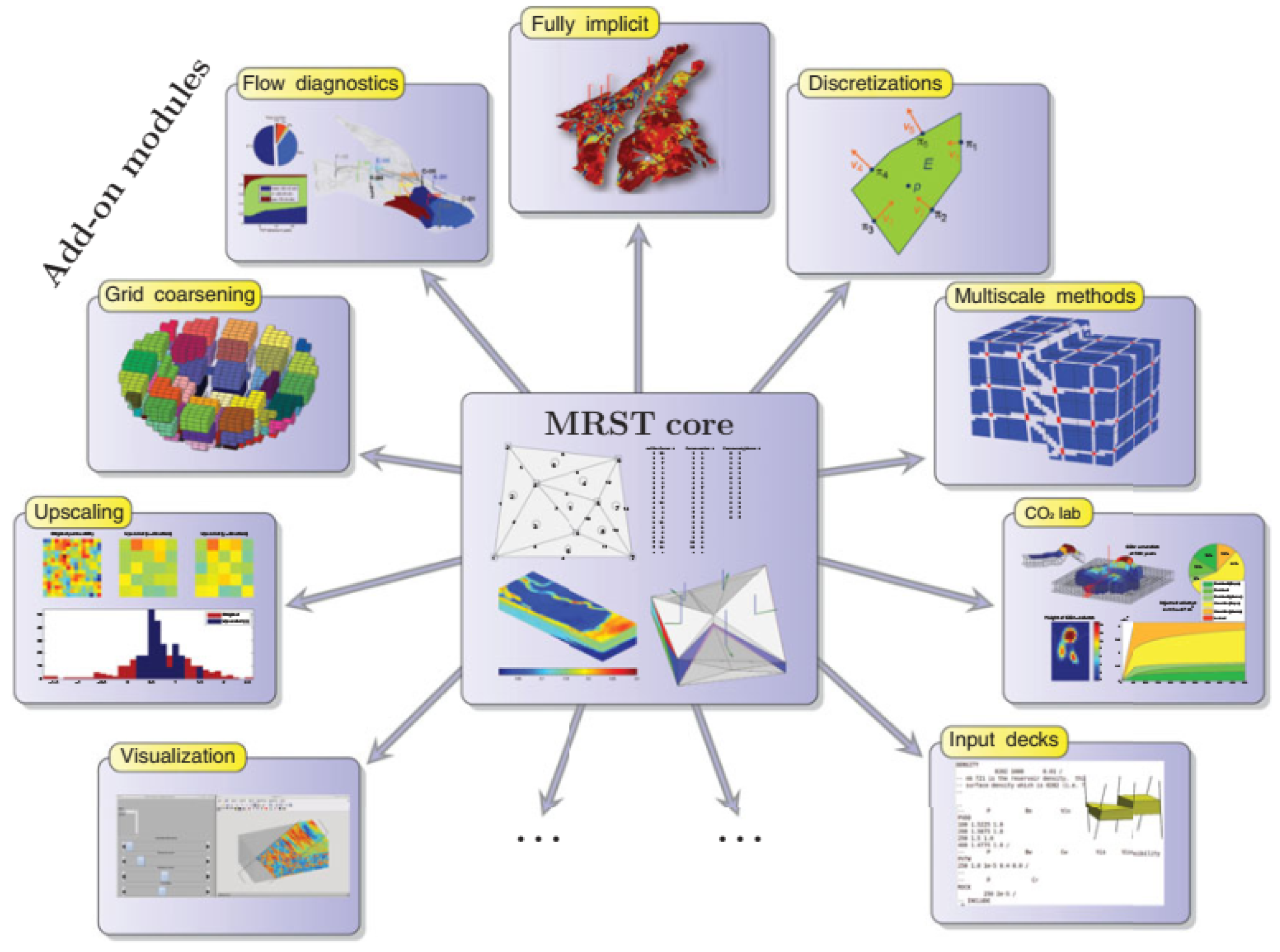
The goal of the MRST research tool is to facilitate investigations into the modeling and simulation of flow in porous media. With a large range of mathematical models, computational techniques, visualization tools, and utility routines, this program improves MATLAB for reservoir modeling. The program’s structure is similar to that of MATLAB, as shown in
Figure 1, with supplementary modules added to enhance its versatility in addition to a core set of procedures [
18].
2.2. Vertical Equilibrium
The first idea for the use of the vertical equilibrium model in reservoir simulation was devised by Coats et al. [
19]. Because CO
2 is so mobile, it can travel large distances when injected into porous rock formations. It is also possible that vertical migration and two-phase separation are much faster than horizontal migration because a typical saline aquifer chosen to store CO
2 is a thin and slightly inclined formation that expands thousands of kilometers. Therefore, with a large density difference between CO
2 and brine, it can be assumed that vertical fluid segregation is an instantaneous process in comparison to up-dip migration. Accordingly, it clarifies the reason why vertical equilibrium (VE) can be used.
Assuming the system is in vertical equilibrium, analytical formulas can be used to estimate the vertical distribution of fluid phases in a vertical equilibrium model. Integrating the flow equations within the vertical plane makes it possible to create a 2D model rather than a 3D one, which drastically lowers the number of grid cells and computational time.
A fully implicit discretization is used in the numerical formulation of MRST-co2lab. This is a sensible decision since it enables the integration of commercial simulators with vertical equilibrium (VE) models to create hybrid models. These techniques work especially well for properly modeling steady-state flow and capturing different trapping processes throughout the long-term CO2 migration.
2.3. Reservoir Model
A revised model for the Johansen formation was presented by Sundal et al. [
13] based on the research, data collection, additional mineralogical samples, and well re-interpolation. This paper makes use of the updated model.
The Johansen Formation, which is topped by the Cook Formation, is the study’s primary location for CO
2 storage. The Horda platform has been drilled by 16 exploration wells, including those in Smeaheia, the Troll field, and the Aurora site (research area). To obtain more information on the Johansen Formation, a well known as the Eos confirmation was drilled in 2019. Eos well data is accessible through Equinor Open Data, and well-log measurements and core data are included in Gassnova [
20] intermediate report on the Johansen Formation.
The wetting phase is brine or the formation water, and the non-wetting phase is CO2. The PVT tables for these phases are based on CO2 and brine properties at a constant reservoir temperature of 98 °C for simplicity, even though the density, viscosity, and formation volume factor of both phases vary with pressure.
The formation volume factor is used to convert the densities of water and CO
2 at surface conditions—1050.48 kg/m
3 and 1.87 kg/m
3, respectively—to their densities under reservoir conditions. Although capillary pressure significantly affects the migration of the CO
2 plume, its impact is not considered in this study due to the lack of reliable experimental data on capillary pressure. This aspect should be addressed in future research [
21].
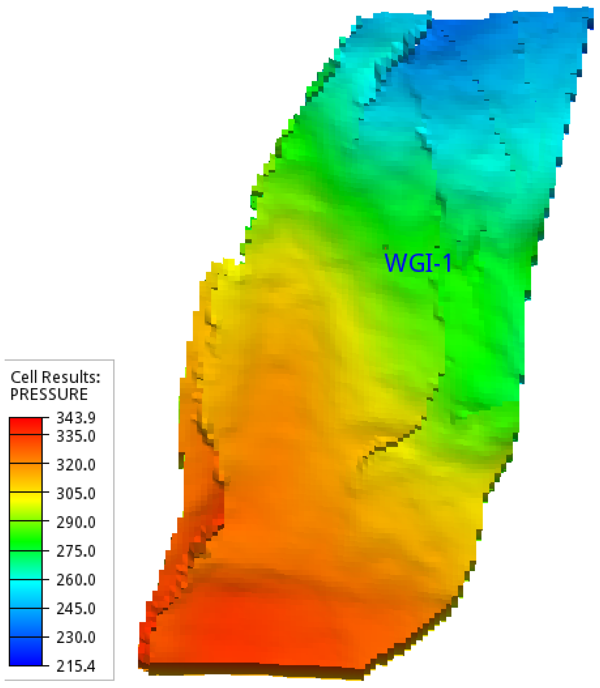
Given the equilibrium state of the Johansen–Cook formations, the initial pressure is 260 [bar] at a datum depth of 2600 m. Analyzing the pressure prior to, during, and following the injection procedure is a crucial part of the CO
2 injection research. The initial pressure distribution and injection well location in the Aurora model are shown in
Figure 2.
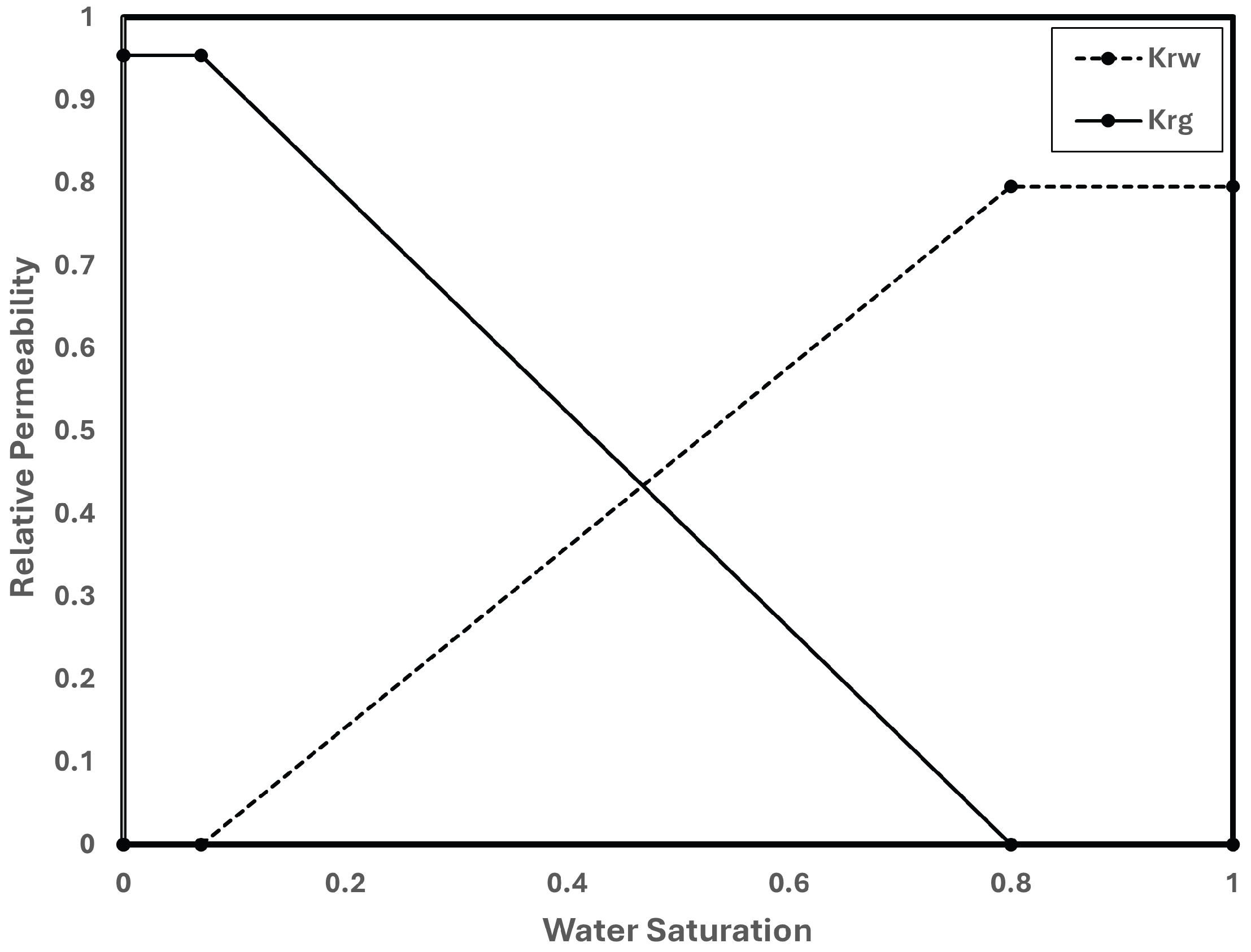
The residual gas saturation in the fluid model is set at 0.2 and the irreducible water saturation at 0.07.
Figure 3 shows the relative permeabilities that were used in this investigation.
The Svarta fault borders the Aurora zone to the west and the Tusse fault to the east. This model is a component of the Johansen Formation, which has porosity values ranging from 7.3 to 31.4 percent and permeability ranging from 0.1 to 500 millidarcy (mD) [
13,
22]. Aurora is also located close to the Troll West fault. Several intra-block faults overlap the storage complex in the Aurora model as well [
23]. Though more analysis and research are required, recent assessments of the faults at the Aurora site indicate that the eastern and north-eastern dipping intra-block faults are expected to impede fluid flow more severely than other faults [
24].
Two injection wells were part of the original Aurora model, located in the southernmost areas. To enable comparability with the Eclipse model, this was changed to a single injection well (WGI-1) since when we have several injection wells, plume analysis becomes more complicated. As a result, the northern part of the reservoir now has a single injection well that runs vertically across the whole thickness of the aquifer. Furthermore, 1.5 million tons of CO2 are injected each year.
There are 1,216,800 cells in the grid (78 × 130 × 120), 747,890 of which are active cells. The cornerpoint structure from the Petrel SE software platform is used in the grid format. A comprehensive overview of all the static and fluid model properties for the Aurora injection location can be found in
Table 1. The injection procedure takes place over a period of thirty years, and the migration of the CO
2 plume that results has been studied for about five centuries.
2.4. MRST Relative Permeability and Capillary Pressure Definition
It is necessary to upgrade the relative permeability model because MRST uses the vertical equilibrium method to transform the 3D model into a 2D one. The upscaled relative permeability model and capillary pressure in MRST can be defined using the following methods:
- 1.
simple: sharp-interface model with linear relative permeabilities, no residual saturation, and vertically homogeneous rock.
- 2.
integrated: sharp-interface model with linear relative permeabilities. This option allows vertically heterogeneous rock and the impact of caprock rugosity.
- 3.
sharp interface: sharp-interface model with linear relative permeabilities and vertically homogeneous rock. It includes the impact of caprock rugosity.
- 4.
linear cap: Linear capillary fringe model with Brooks–Corey type relative permeability and endpoint scaling.
- 5.
S table: capillary fringe model based on sampled tables in the upscaled saturation parameter.
- 6.
P-scaled table: capillary fringe model based on sampled tables in the upscaled capillary pressure parameter.
- 7.
P–K-scaled table: capillary fringe model based on sampled tables in the upscaled capillary pressure parameter and taking variations in permeability into account through a Leverett J-function relationship.
These many relative permeability models are described in detail by Nilsen et al. [
25]. Since Eclipse also uses a table for relative permeabilities, the default relative permeability model in MRST, known as the “P-scaled table,” has been adopted in this investigation. As a result, the relative permeability has been defined using the “P-scaled table”. In order to find a more appropriate relative permeability model, it is highly recommended to investigate alternative possibilities in further research.
2.5. MRST and Eclipse Model Comparison
The shape of the CO2 plume is the main focus for comparing the CO2 plume migration patterns between the MRST and Eclipse models. For comparison, the gas saturation distribution from the 3D Eclipse model must be translated to a 2D grid model since the VE MRST-co2lab delivers findings in that format. By averaging the gas saturation for each column in Eclipse according to the pore volume of each cell in the column, this conversion is accomplished. To calculate the averaged gas saturation, the pore volumes and gas saturations of each cell are multiplied together, and the total of these products for each column is then divided by the column’s total pore volume. This procedure makes it possible to compare the 2D MRST model with the 3D Eclipse model.
While analyzing the MRST grid model, one discrepancy has been detected. The vertical equilibrium (VE) averaging mechanics in the MATLAB Reservoir Simulation Toolbox (MRST) are mainly responsible for the fluctuation in pore volumes throughout certain sections of the model, as seen in
Figure 4-Left. Any vertical stack of grid cells with at least one active cell at the top is referred to as an active column, and MRST finds them in the VE simulation. But when active cells are ignored in a column below the final inactive cell, something goes wrong. The dramatic variances seen in the model can result from this cell removal, which can lead to considerable inconsistencies in the representation of pore volume. Accurately evaluating the VE simulation findings and resolving any related model setup errors require an understanding of this mechanism.
The blue zones (
Figure 4-Left), which have the lowest pore volumes, are discovered to have inactive cells in the middle layers after the active columns in the model were examined. As a result, MRST removed the active cells that were layered over by the inactive ones. Therefore, these zones’ average pore volume is much smaller than the grids’ surrounding ones. As seen in
Figure 4-Right, this was addressed by altering the average pore volumes method determined by the standard vertical equilibrium (VE) averaging method in MRST.
It should be mentioned that internal faults cannot be detected in the VE model used in the current version of MRST, resulting in the difference in the plume shape between MRST and the Eclipse simulator, since the boundaries and internal faults have vital effects on permeabilities.
Next, we compare the fluid models to make sure the model was correctly transferred after importing and modifying the grid model from Eclipse to MRST. This entails comparing the matching values and correlations found in MRST with the densities and viscosities of water and CO2 defined in Eclipse.
The following formulas are commonly used by MRST to define fluid density and viscosity:
in which
[kg/m
3] and
[Pa.s] are density and viscosity at reservoir pressure and temperature, respectively;
[kg/m
3] and
[Pa.s] are the density and viscosity at reference condition, which should be defined in MRST, c [bar
−1] is compressibility; and p [bar] and
[bar] are the reservoir and reference pressure, respectively. Since the fluid model in Eclipse is a black-oil model, the reservoir temperature is assumed constant, 98 °C, as mentioned in
Table 1.
2.6. Sensitivity Analysis
To assess the uncertain parameters in reservoir modeling, such as porosity, permeability, and relative permeability curve, several simulation runs are required in order to analyze the risk in CO2 storage projects.
Several simulation runs are required to assess the uncertain parameters in reservoir modeling, such as porosity, permeability, and relative permeability curves. This method aids in the analysis of the risks relating to CO2 storage projects.
This work presents a sensitivity analysis of five uncertain parameters and their effects on injection pressure, distribution of the CO2 plume, and amounts of CO2 stored by different mechanisms. The five variables that were examined are as follows:
- 1.
Porosity;
- 2.
Permeability;
- 3.
Residual Gas Saturation;
- 4.
Rock Compressibility;
- 5.
Relative Permeability Curve.
3. Results and Discussion
3.1. Relative Permeability Models Comparison
The relative permeability of the gas utilized in MRST and Eclipse is displayed in
Figure 5. A polynomial function is defined in MRST to fit the Eclipse model, whereas Eclipse employs a table of relative permeability versus saturation. There is no denying how well these two models match.
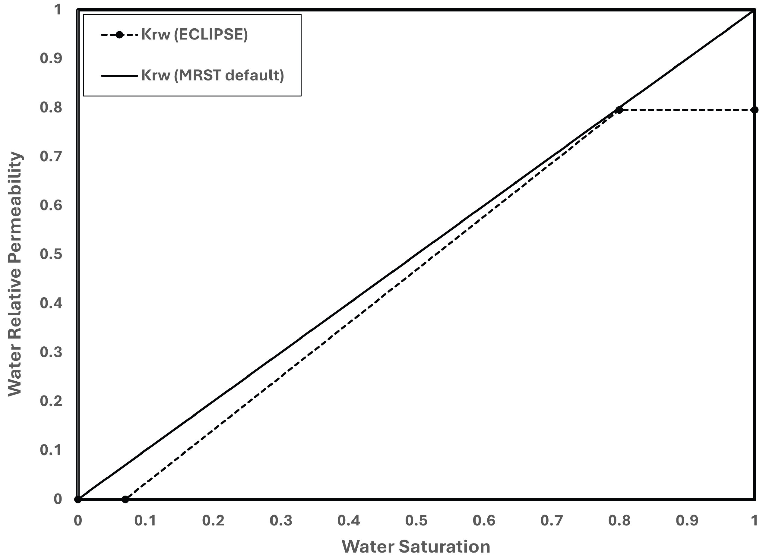
The water relative permeability model in MRST and Eclipse is displayed in
Figure 6. With zero irreducible water and residual gas saturations, the default water relative permeability in MRST is a linear function of saturation with a slope of one. Eclipse, on the other hand, has residual gas saturation and irreducible water saturation values of 0.2 and 0.07, respectively.
Since both the irreducible water and residual gas saturations are set to zero, it initially looks like the MRST water relative permeability does not match the Eclipse model. To be used in the relative permeability model, the residuals are defined in the MRST main script code. Because it takes these residuals into account, the default MRST relative permeability model does, in fact, match the Eclipse model.
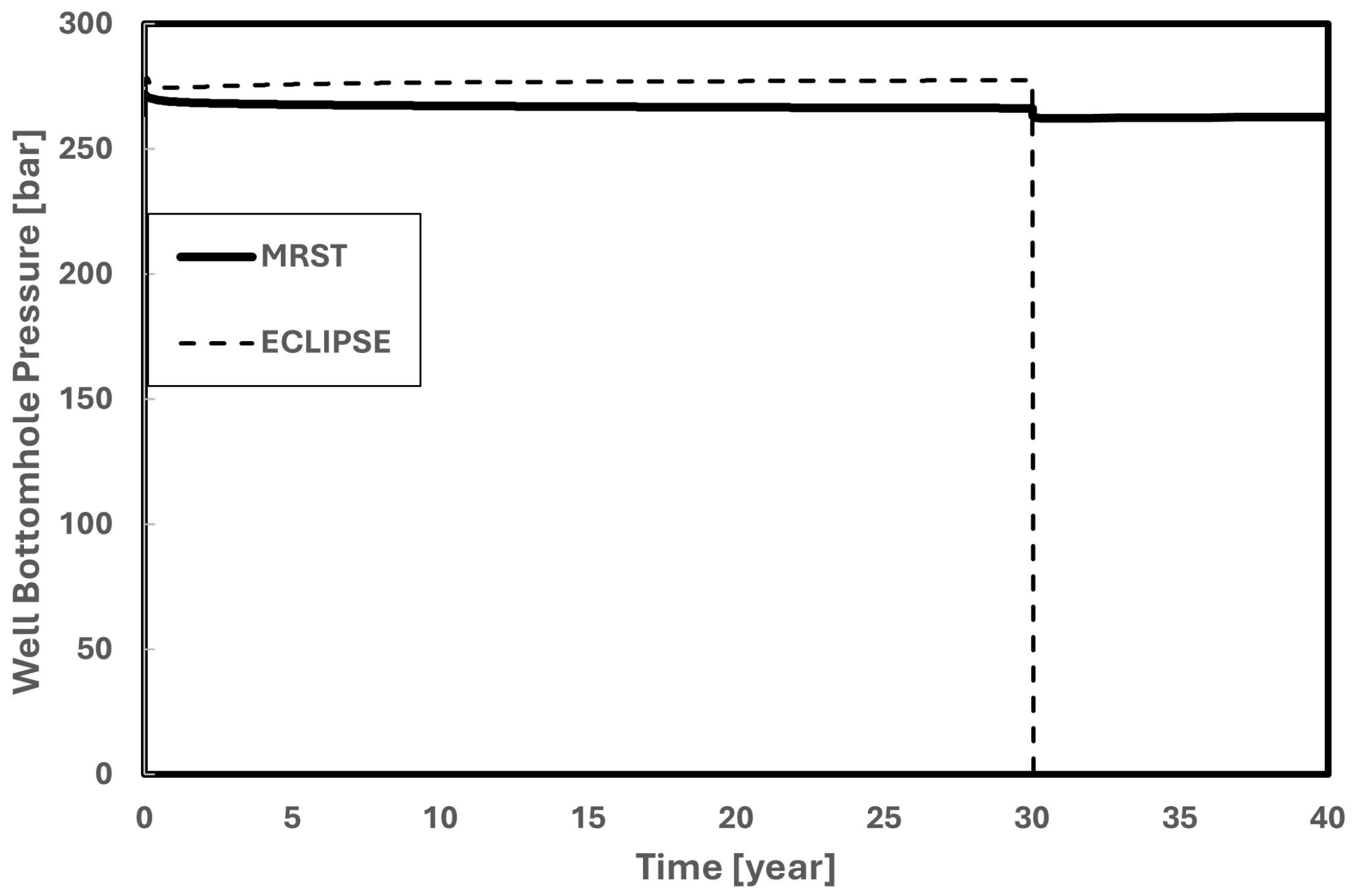
3.2. Initial Pressure Comparison
The initial well bottom-hole pressure in MRST is different from that in Eclipse at the onset of CO
2 injection. In this work, the discrepancy is examined and reconciled. It is crucial to first make clear how pressure is initialized in MRST. MRST uses the following formula to determine each grid block’s pressure under reservoir conditions:
in which
p is the pressure of each grid block in the reservoir model in [Pa],
is water density in [kg/m
3] at reservoir condition,
g is the gravity factor in [m/s
2], and
h is the depth of each grid block in the reservoir model in [m].
Analysis revealed that the problem stemmed from the water density that was utilized in the MRST. The water density was reconstructed using the Eclipse initial pressure since the initial pressure in MRST and Eclipse should be equal. The pressure initialization problem was fixed by adjusting the MRST water density to 1020.19 [kg/m
3], as seen in
Figure 7. For the first thirty years of injection, there are small differences in well bottom-hole pressure between MRST and Eclipse. When the injector wells are closed after 30 years, the Eclipse pressure falls to zero and the MRST displays a steady pressure of about 260 [bar].
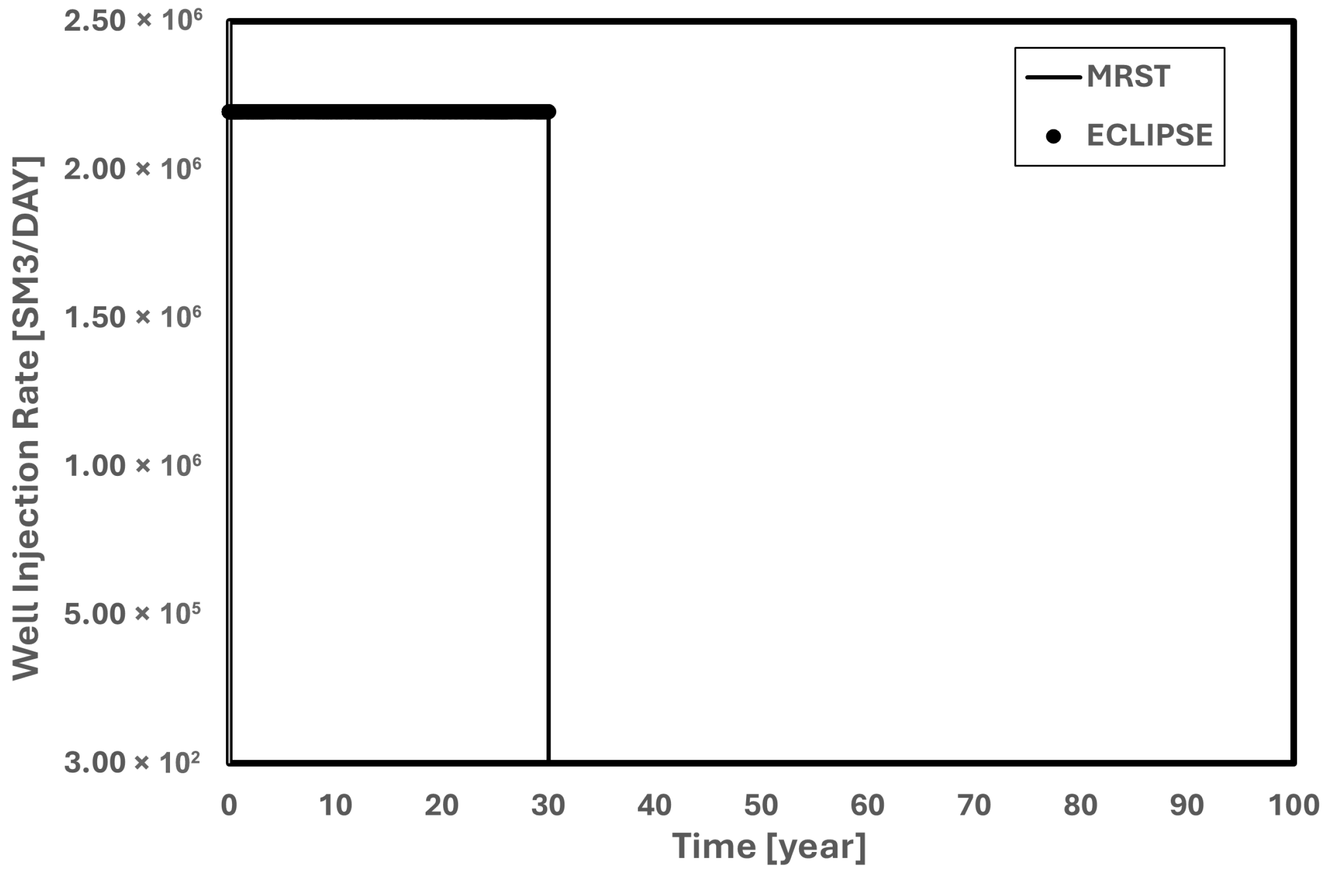
3.3. Injection Rate Comparison
To ensure that the injection rates in MRST and Eclipse are the same,
Figure 8 compares this parameter. It is evident that the injection rates in MRST and Eclipse are the same throughout the injection time.
3.4. MRST and Eclipse PVT Model Comparison
It is crucial to first define the range of pressure changes before and after injection before comparing PVT models.
Figure 9 illustrates the pressure variation range of 220–320 [bar] that occurs both during and after the injection time. Consequently, within this pressure range, the PVT models in Eclipse and MRST should be aligned.
Equation (
1) and (
2) for density and viscosity calculations should be applied using the Eclipse PVT model to establish the MRST CO
2 compressibility. As demonstrated in Equation (4), CO
2 compressibility is determined at each pressure using Equation (
4) because it is not specifically mentioned in the Eclipse data file.
in which
[bar
−1] is CO
2 compressibility;
and
[Rm
3/Sm
3] are gas formation volume factor at the reservoir and reference conditions, respectively; and
and
p [bar] are the reference and reservoir pressure, respectively.
In MRST, density and viscosity are computed using a reference pressure of 300 [bar]. Therefore, in order to compute density and viscosity in Equations (1) and (
2), the water and gas compressibility should be chosen at this reference pressure.
Figure 10 shows that at 300 [bar], the CO
2 compressibility utilized in the Eclipse model is roughly
[bar
−1].
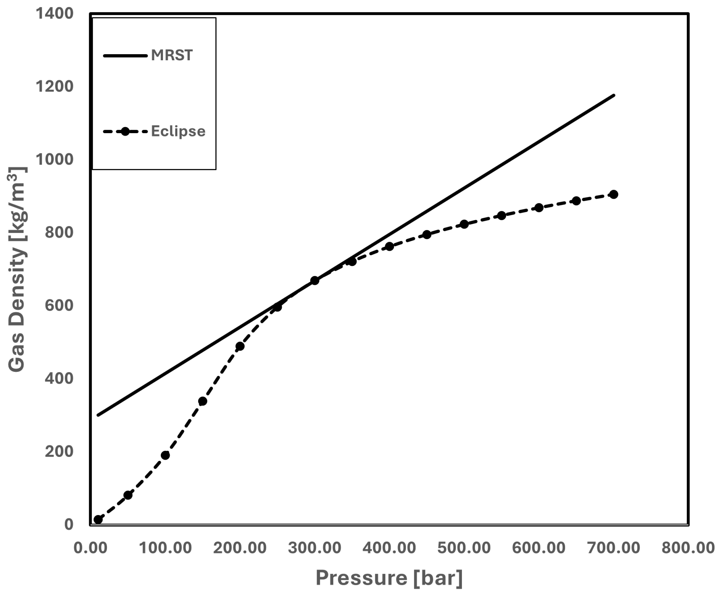
The CO
2 density models employed in MRST and Eclipse are compared in
Figure 11. Since the MRST model calculates densities at different pressures using Equation (
1), it is linear in contrast to the non-linear CO
2 density model found in Eclipse. It is crucial to remember that Equation (
5) is used to calculate CO
2 density because the Eclipse data file lacks clear density information.
in which
[kg/Rm
3] is CO
2 density at reservoir condition,
[kg/Sm
3] is CO
2 density at surface condition, and
[Rm
3/Sm
3] is CO
2 formation volume factor.
Figure 11 makes it clear that, in the 220–320 [bar] injection pressure range, the CO
2 density in Eclipse and MRST is almost the same.
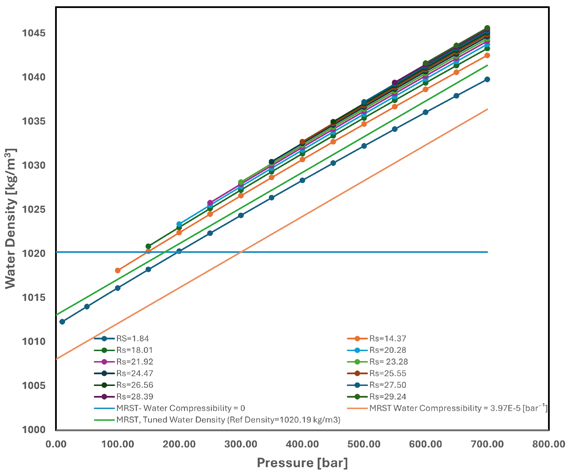
The water density model in MRST has been defined using the same methodology as the gas density model. First, using Equation (
6) from the Eclipse PVT model, the water compressibility, which must be used in Equation (1), is computed for different solution gas–water ratios (
), as illustrated in
Figure 12:
in which
[bar
−1] is water compressibility;
and
[Rm
3/Sm
3] are water formation volume factor at the reservoir and reference conditions, respectively; and
and
p [bar] are the reference and reservoir pressure, respectively.
The water compressibility at a reference pressure of 300 [bar] is roughly
[bar
−1], as
Figure 12 illustrates. This compressibility number can be utilized to find the water density in MRST using Equation (
1). A comparison of the water density models in MRST and Eclipse is shown in
Figure 13.
There is still a small difference between the average Eclipse water density and the MRST water density (including water compressibility) even though the MRST water density and water compressibility at the reference pressure are chosen correctly based on the updated pressure initialization and the Eclipse PVT model. A 5 kg/m3 adjustment is made to the final water density model in MRST in order to reduce this gap, which produces results more in line with the Eclipse data.
It is significant to note that Equation (
7) is used to compute the water density because the Eclipse data file lacks clear density information:
in which
[kg/Rm
3] is the water density at reservoir condition,
[kg/Sm
3] is the water density at the surface condition,
[Sm
3/Sm
3] is the solution gas–water ratio,
[kg/Sm
3] is the CO
2 density at surface condition, and
[Rm
3/Sm
3] is the water formation volume factor.
A comparison of the CO
2 viscosity models in Eclipse and MRST at different pressures is presented in
Figure 14. While CO
2 viscosity in Eclipse is directly retrieved from the explicitly provided data file, in MRST it is computed using Equation (
2) with the known CO
2 compressibility value. Both viscosity models are almost the same in the injection pressure range of 220–320 [bar].
Moreover, the Eclipse water viscosity model and the MRST water viscosity, which takes water compressibility into consideration, are matched quite well, as
Figure 15 illustrates. It is also important to remember that the Eclipse viscosity model is taken straight from the data file, whereas the MRST water viscosity is determined using Equation (
2), which is based on the known water compressibility value.
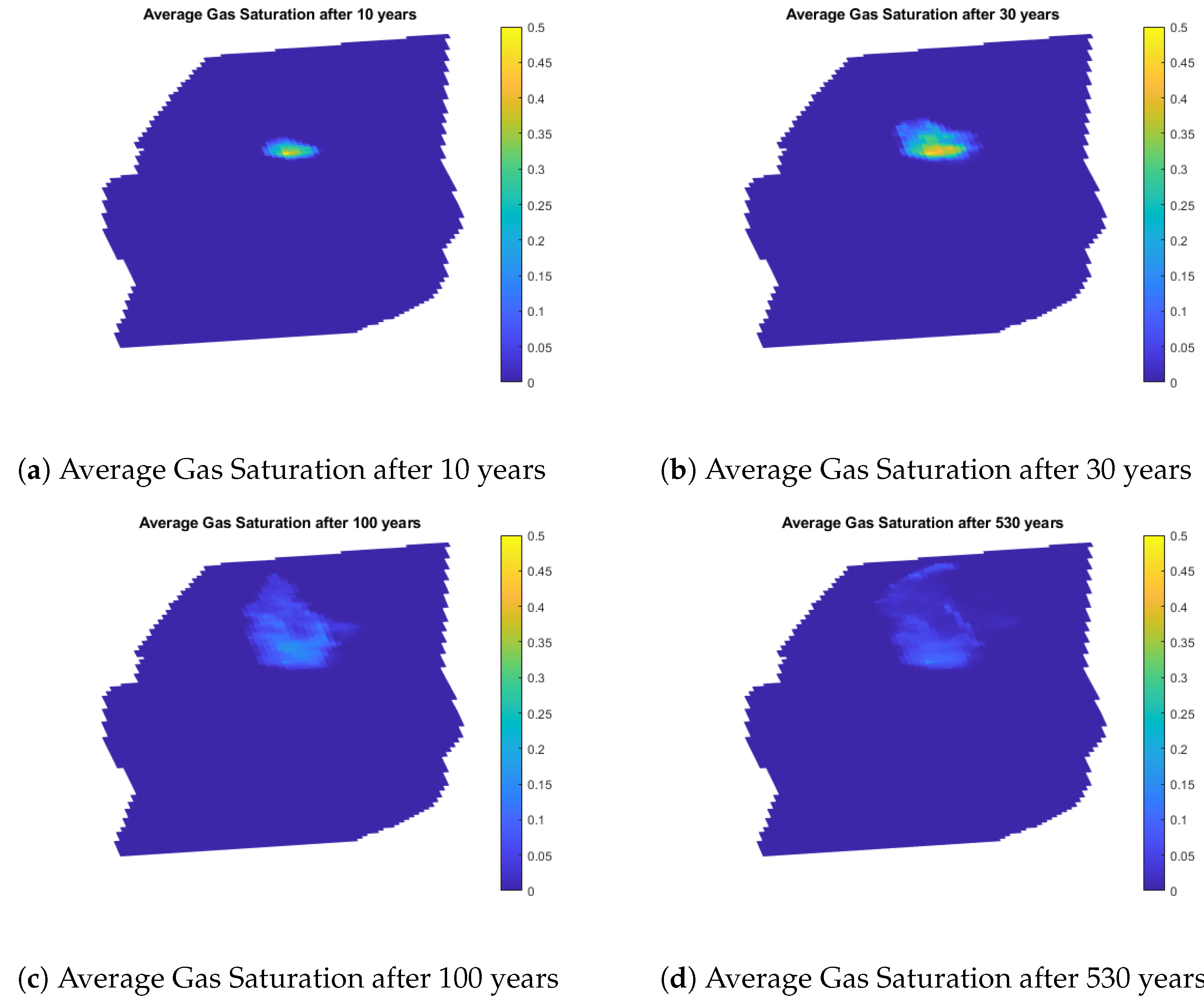
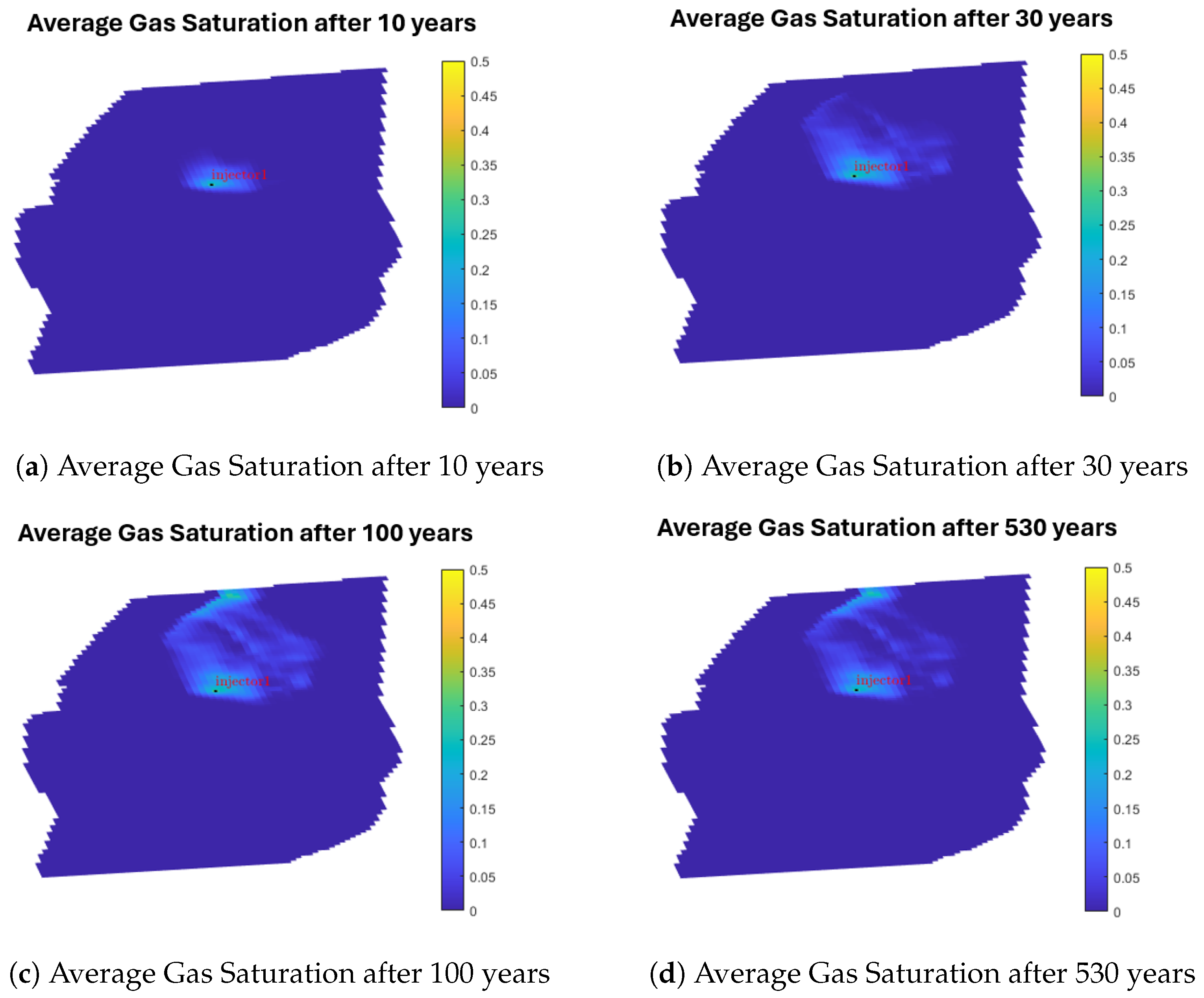
3.5. CO2 Plume Comparison
The development and motion of the CO
2 plume in Eclipse and MRST, respectively, are shown in
Figure 16 and
Figure 17. The plume can be seen in the top images (a and b) after 10 and 30 years of injection, and in the bottom images (c and d) after the injection has stopped for 70 and 500 years. Compared to MRST, Eclipse exhibits a more rounded plume shape after ten years. Furthermore, the CO
2 saturation in the vicinity of the injection well in Eclipse (∼0.45) is greater than that in the vicinity of the well-bore in MRST (∼0.25), and the plume morphology in MRST is broader than in Eclipse. Thirty years later, the near-well-bore CO
2 saturation in both Eclipse and MRST is relatively unaltered when compared to the 10-year CO
2 migration, even though MRST continues to create a more diffused plume morphology than Eclipse.
The injection process is stopped after 30 years, and over the next 500 years, CO2 migration is observed. After 100 years, there is a noticeable difference between the plumes (70 years post-injection). While CO2 saturation near the well-bore declines in both MRST and Eclipse, the MRST plume is significantly wider than the Eclipse plume. The MRST plume has stretched to the border, indicating accumulated CO2 saturation in that area, whereas the CO2 plume in Eclipse has not yet reached the boundary.
In general, for every time interval, the MRST plume is consistently substantially wider than the Eclipse plume. This discrepancy is primarily due to “Reservoir Heterogeneity”. As noted, using the vertical equilibrium approach, the MRST co2-lab computes the vertical average of reservoir model parameters including porosity and permeability. The single-layer averaged MRST model shows more permeability in the x and y directions than the upper layers of the Eclipse reservoir model, which is important for CO2 movement. This is because the permeability in the upper layers of the Aurora reservoir model is significantly lower than in the lower levels. As a result, the Eclipse plume is much narrower than the MRST plume. Reservoir heterogeneity has a much greater impact on the differences in plume forms, even though other factors like relative permeability curves and end-point upscaling may also play a part.
The free plume, which stores around 30 MT of CO
2, is the main storage mechanism for the first 50 years, as illustrated in
Figure 18. Residual and dissolution mechanisms come next. The free plume disappears after about 200 years as a result of exiting CO
2 from the reservoir before year 50. After that, the amount of dissolved CO
2 keeps rising while the amounts of residual CO
2 and CO
2 that has left the reservoir stay constant. In the end, 530 years later, 27 [MT] of CO
2 left the reservoir border, while roughly 18 [MT] (1 [MT] =
[kg]) of CO
2 is still held in the reservoir due to residual and dissolving processes.
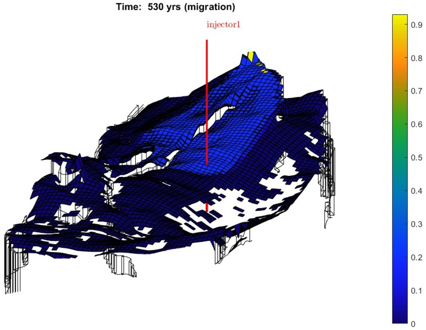
The capacity of MRST vertical equilibrium to use analytical capillary pressure equations in order to transform a 2D model into a 3D model is one of its primary features. The 3D CO
2 saturation produced from the 2D model made with the MRST vertical equilibrium feature is shown in
Figure 19. Due to the geological upward slope, the gas plume is spread toward the northern portion of the model in this three-dimensional image. This 3D figure also shows a fault that is located to the north of the injection well and runs from south to north.
The VE application in this model decreased the simulation time significantly. The Eclipse simulation requires approximately 1 day, but MRST completely the same simulation in about 15 min—approximately 100 times faster.
3.6. Sensitivity Analysis
Five unknown factors are subjected to a sensitivity analysis in this section: the relative permeability curve, rock compressibility, residual gas saturation, porosity, and permeability. These parameters’ impacts on CO2 plume morphology, well bottom-hole pressure, and the disintegration of storage devices are depicted.
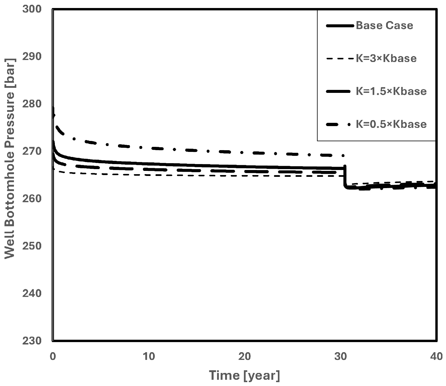
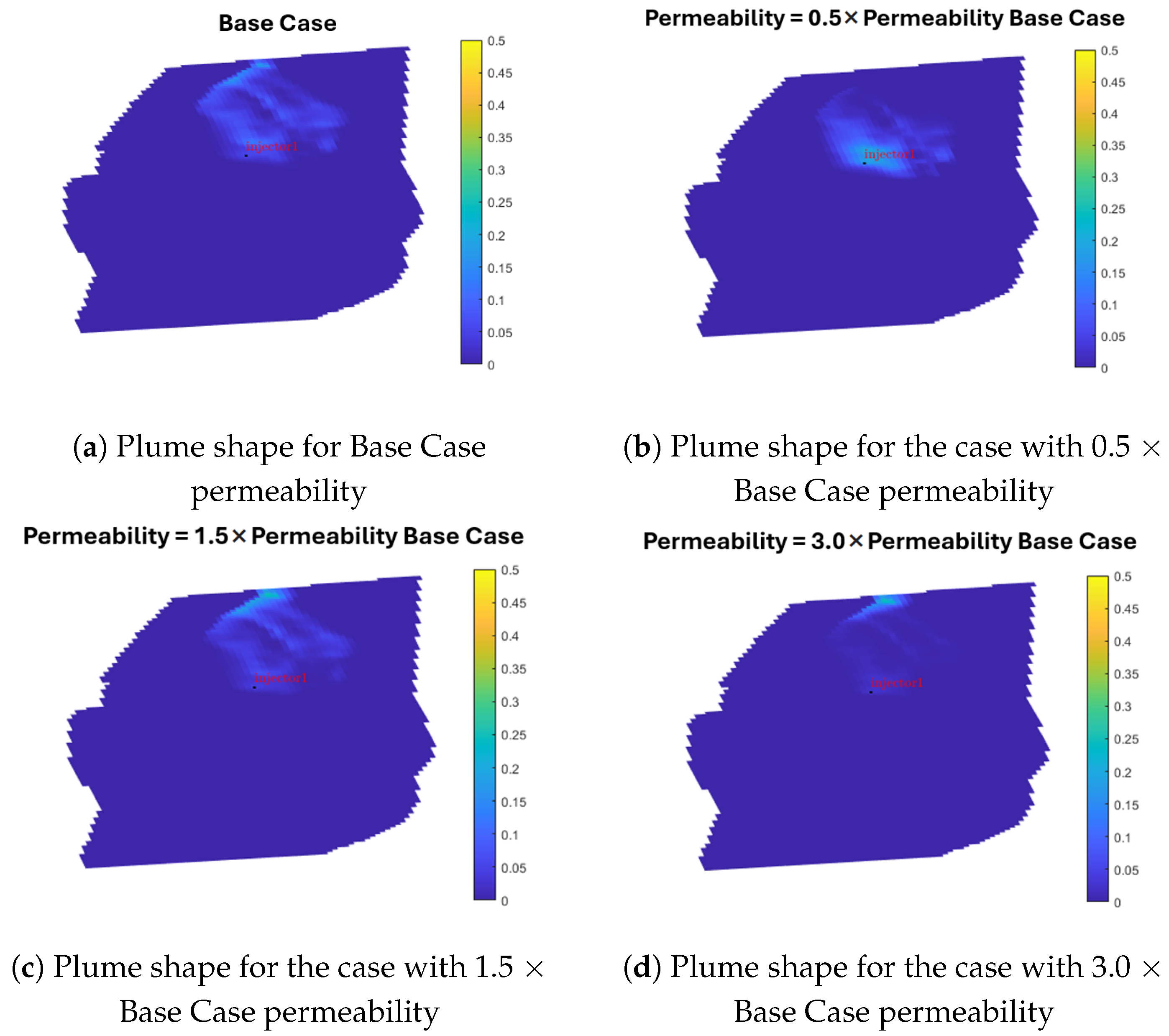
3.6.1. Permeability
The permeability sensitivity analysis is performed on the horizontal permeability because the VE model only takes that into account in the 2D model. For this investigation, three permeability scenarios are chosen: , , and .
The effect of changing permeability on well bottom-hole pressure is seen in
Figure 20. Because of faster pressure dissipation, the well bottom-hole pressure drops as permeability increases. The pressure in MRST returns to the initial bottom-hole pressure of about 260 [bar] once the injection stops at 30 years.
After 50 years,
Figure 21 illustrates how permeability variations impact the structure of the CO
2 plume. Panels c and d illustrate how increasing permeability speeds up plume migration towards the upper boundary, while panel b illustrates how decreasing permeability restricts the plume’s growth. In particular, the near well-bore gas saturation is approximately 0.2 with
, while in the other cases, the same region’s gas saturation is less than 0.1.
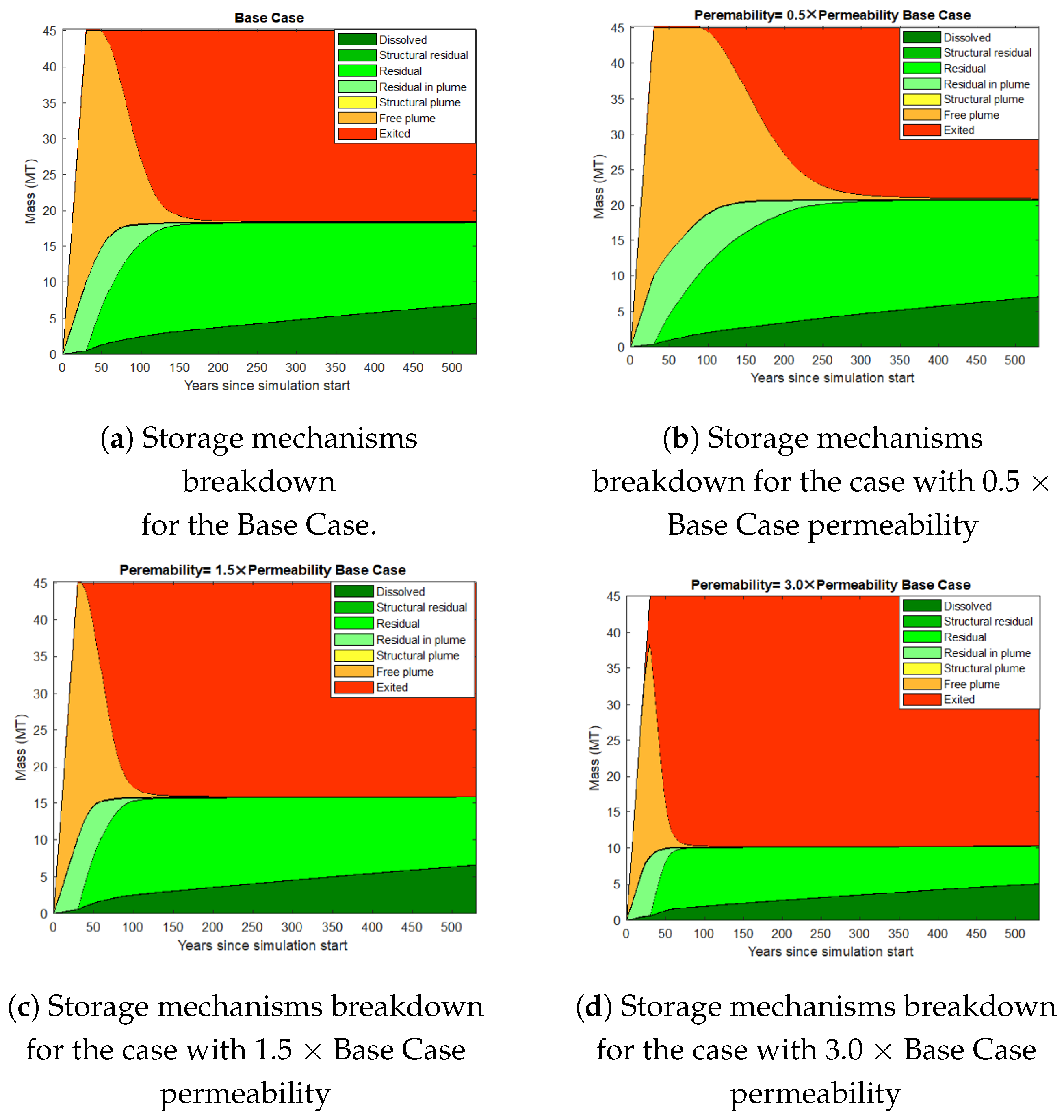
The effects of permeability variations on the disintegration of various storage methods (dissolved, free plume, and residual) after 530 years are depicted in
Figure 22. The main storage mechanisms in all permeability scenarios are residual and dissolved, and since the free plume has left the reservoir model through the upper boundary, it is no longer present. Increased permeability decreases residual storage as expected. This happens because in high-permeability circumstances, the CO
2 plume flows more easily at roughly the same injection pressure, leading to reduced residual storage. Interestingly, compared to residual storage, the amount of dissolved storage is less susceptible to permeability variations.
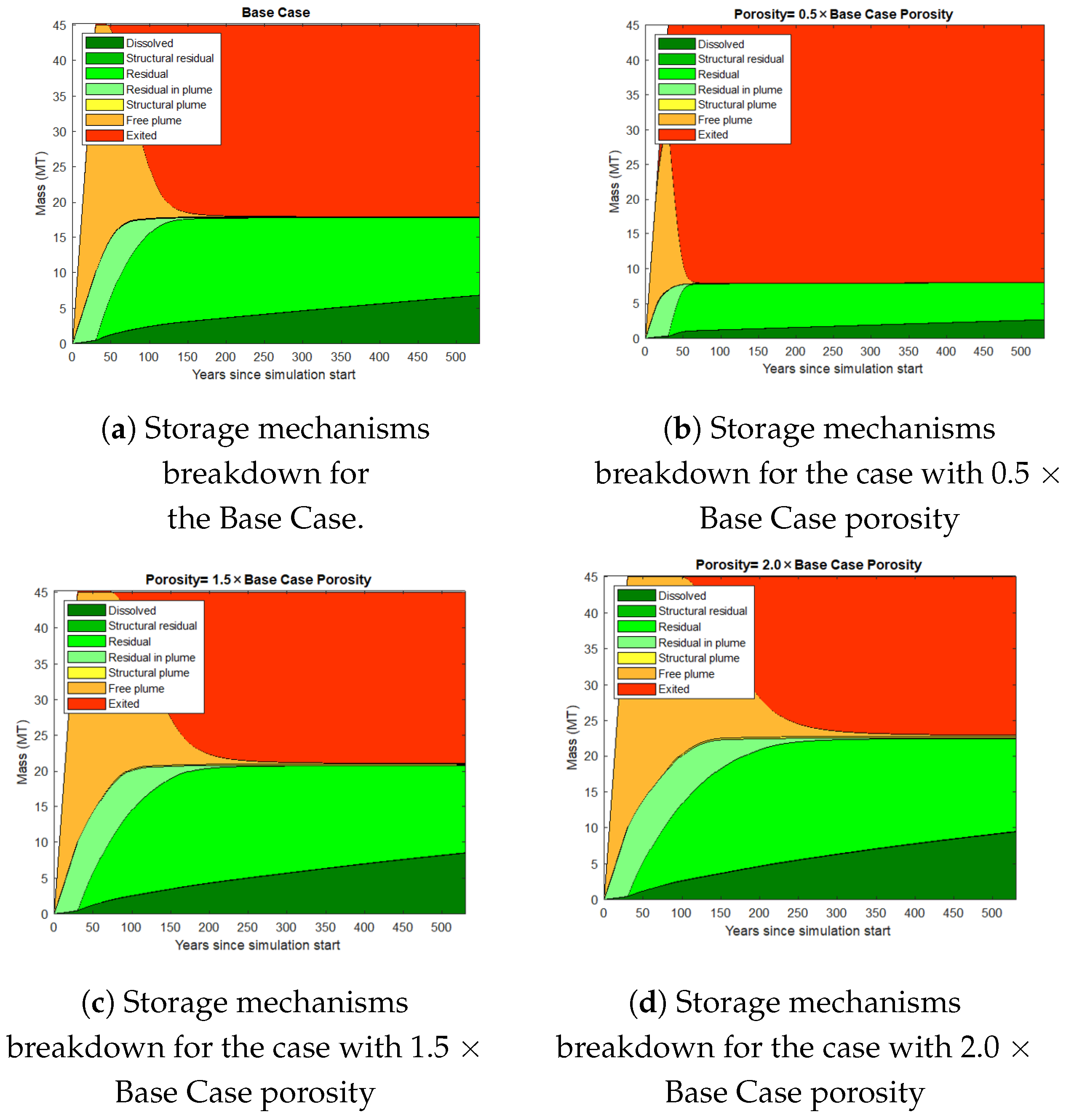
3.6.2. Porosity
Three porosity arrays (, , and ) are chosen to conduct a porosity sensitivity analysis.
Figure 23 shows that plume growth is decreased with increased porosity. This is because higher porosity results in larger pore capacity in each grid cell to retain CO
2, which leads to a less extended plume when the injection rate is kept constant. Furthermore, compared to the base case, gas saturation close to the well-bore is higher in the higher porosity situations (c and d).
In comparison to lower porosity situations (a and b),
Figure 24 illustrates that larger porosity scenarios (c and d) provide more CO
2 storage through residual and dissolved mechanisms. A significant portion of the free plume escapes through the top barrier in the lower porosity instances.
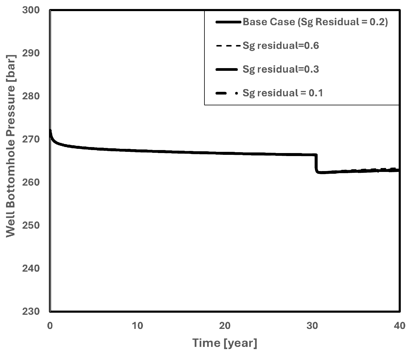
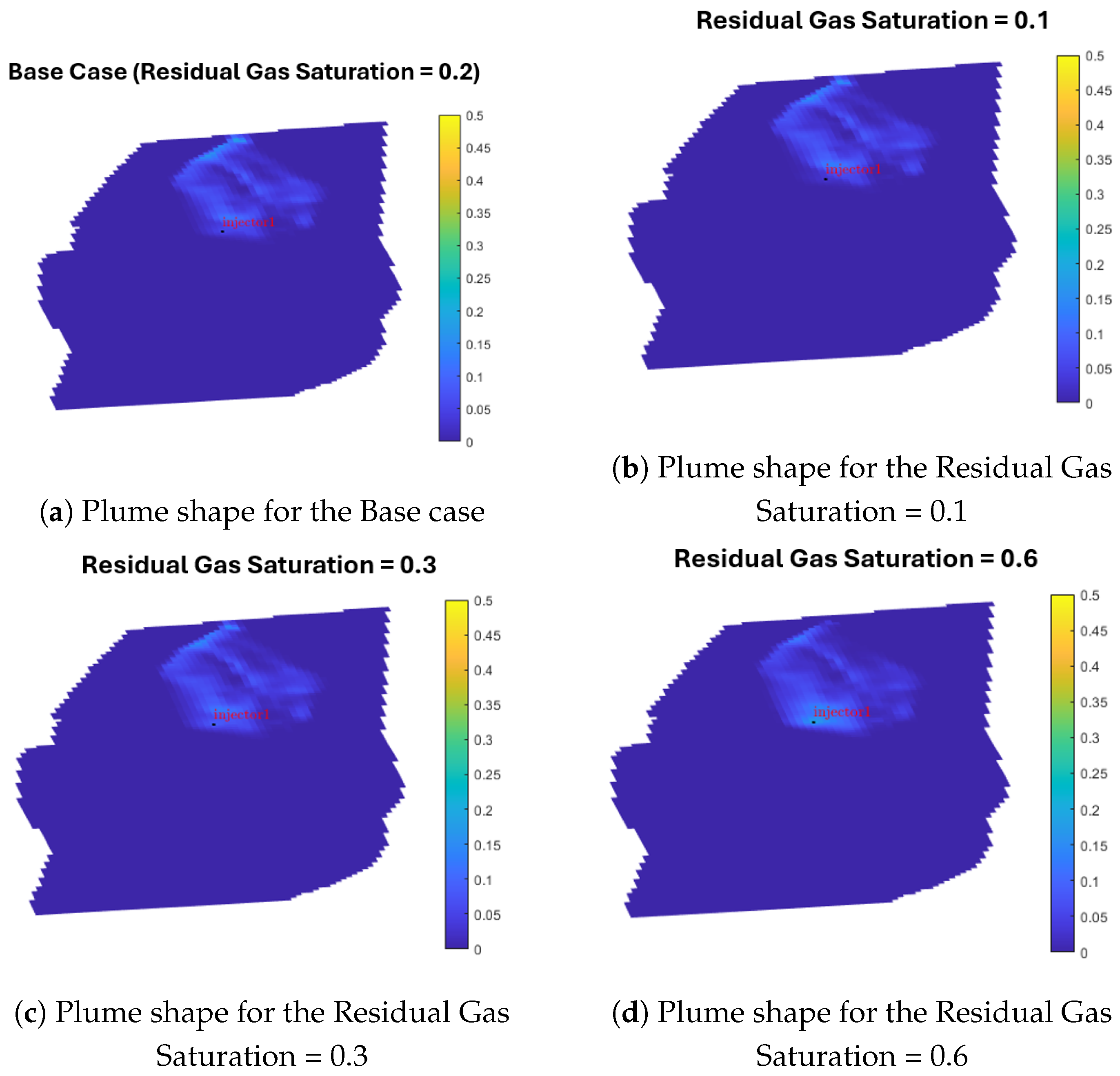
3.6.3. Residual Gas Saturation
To study the sensitivity of the MRST reservoir model to residual gas saturation, the following values have been selected: 0.1, 0.3, and 0.6, in addition to the base case value of 0.2.
Given that the injection pressures in each of the various saturation instances are almost equal,
Figure 25 provides further evidence that the well bottom-hole pressure in the reservoir model is not sensitive to residual gas saturation.
Residual gas saturation influences the CO
2 footprint in the plume form but does not affect injection pressure. Higher residual gas saturation, as seen in
Figure 26, restricts the gas plume’s ability to expand. This is because, in comparison to scenarios with lower residual gas saturation, simulation grids with higher residual gas saturation retain more CO
2, which inhibits the plume from spreading as much.
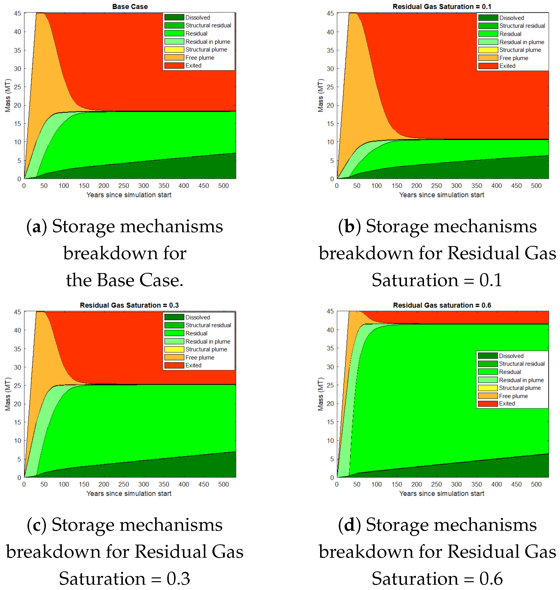
While residual gas saturation does not affect injection pressure or plume shape, it has a major effect on the breakdown of the CO
2 storage mechanism, as
Figure 27 illustrates. This picture shows that increased residual gas saturation increases the quantity of stored CO
2, even though the dissolved storage mechanism contributes in a similar way in each of the three residual gas saturation scenarios. This is because, with greater residual saturations, CO
2, a non-wetting phase, prefers to stay in the grid blocks. Furthermore, the figure unequivocally demonstrates that, in the residual gas saturation sensitivity analysis, residual and dissolved mechanisms are the most efficient storage mechanisms.
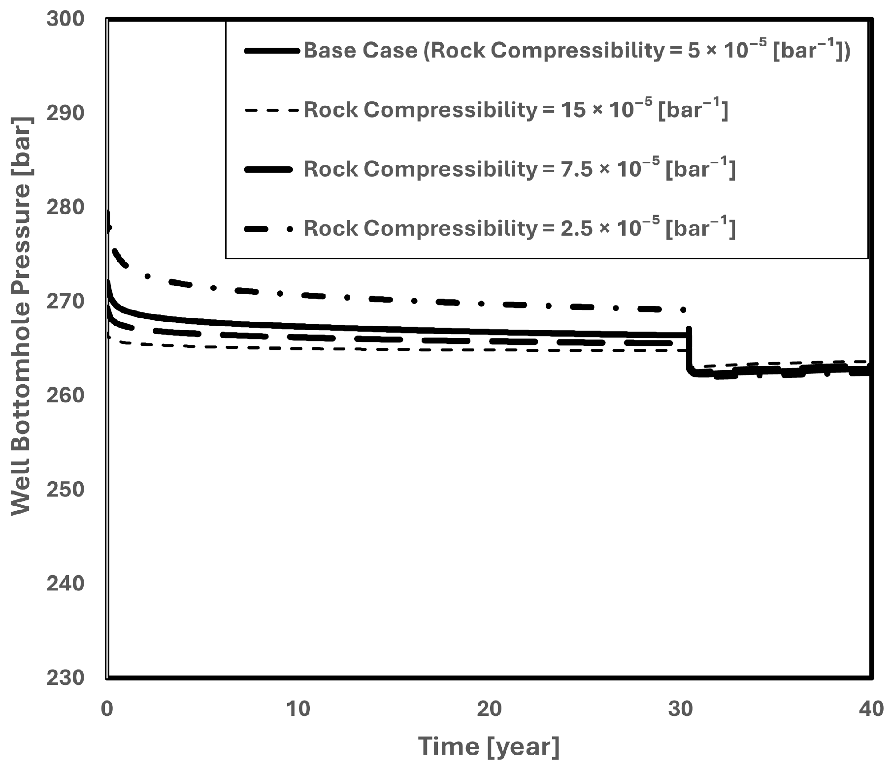
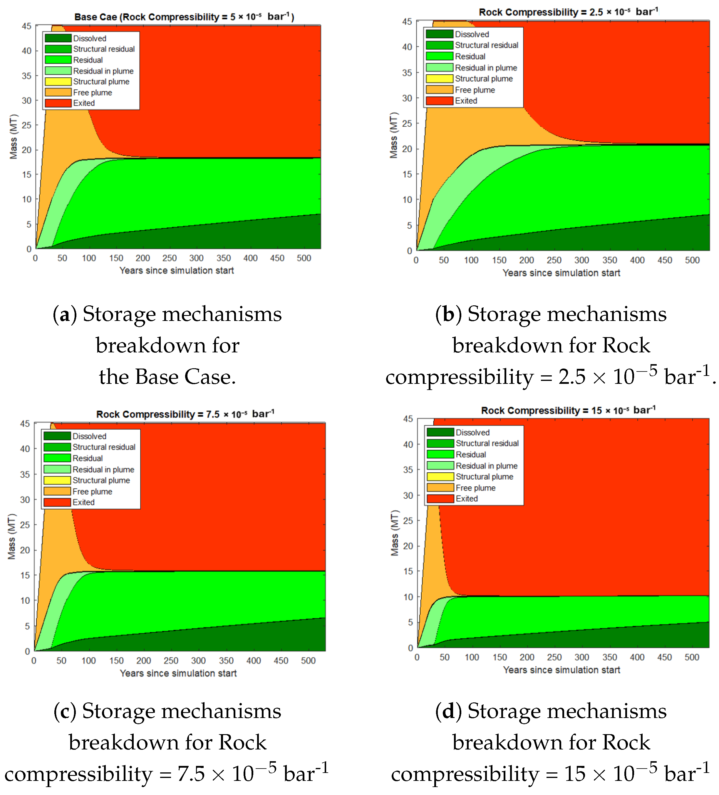
3.6.4. Rock Compressibility
In addition to the base case value of = [], the compressibility of rock is also investigated in the sensitivity analysis with the following values: = [], = [, and = [].
Figure 28 illustrates how a small drop in the bottom-hole pressure is caused by increasing rock compressibility. This happens as a result of the reservoir rock structure’s increased capacity to disperse pressure. High rock compressibility facilitates easier pressure transmission, which lowers injection pressure. In essence, lower compressibility leads to increased injection pressure, whereas higher compressibility functions as a spring to lessen the injection pressure.
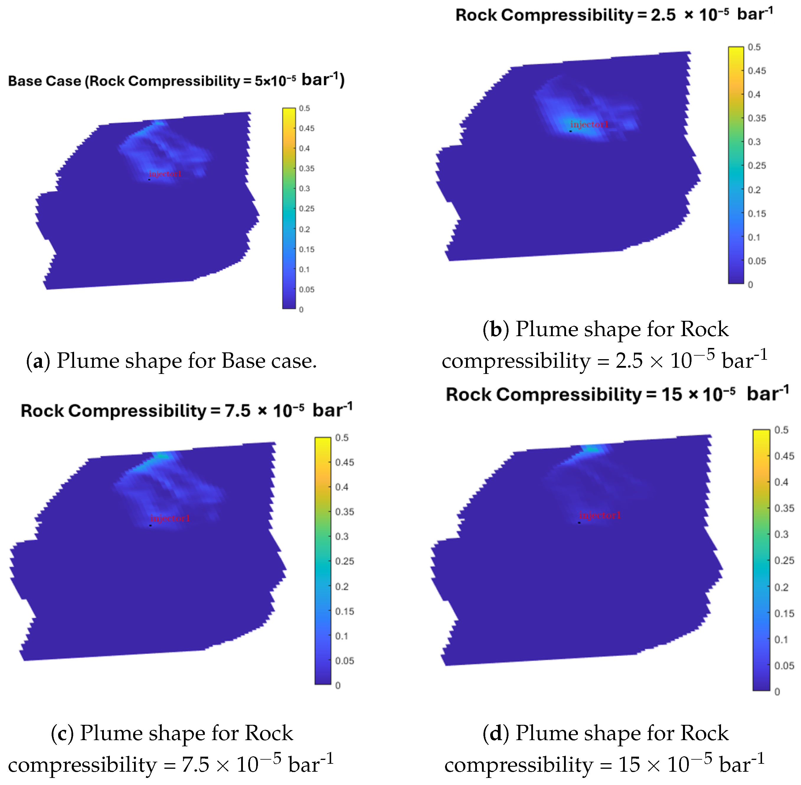
The effect of rock compressibility on the shape of the CO
2 plume is seen in
Figure 29. Higher rock compressibility, as expected, causes the rock to expand and extend the CO
2 plume longer. This results in larger plume dissipation in high compressibility scenarios (d) when compared to other compressibility cases. As a result, as
Figure 30 illustrates, more injected CO
2 leaves the reservoir when the rock is more compressible. This picture also shows that residual and dissolved mechanisms are the main storage mechanisms in the rock compressibility study, just as other sensitivity factors.
Notably, with a rock compressibility of , the rate of free plume evacuation from the upper boundary is highest, as high rock compressibility pushes the plume towards the boundary. As a result, the case with the highest compressibility has the lowest CO2 storage—roughly 10 [MT].
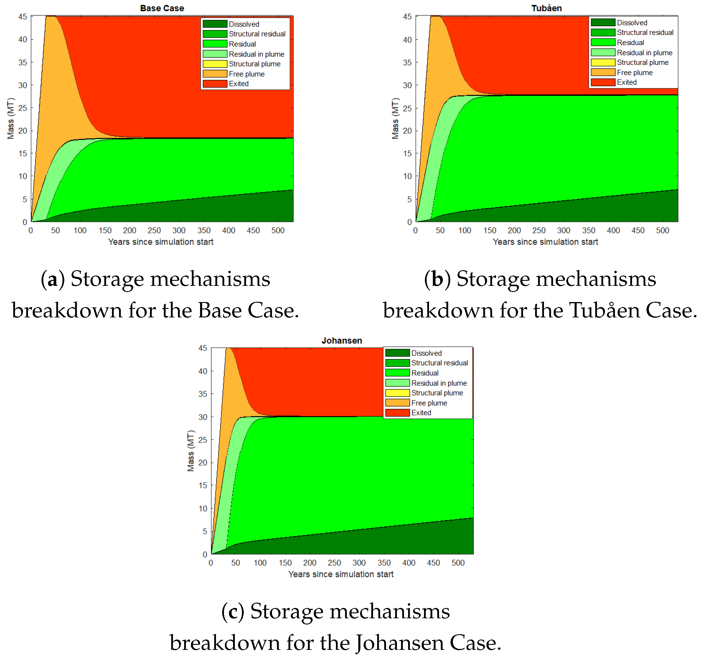
3.6.5. Relative Permeability Curve
The sensitivity study incorporates two relative permeability curves, the Johansen and Tubåen formations, in addition to the base case [
20]. The Utsira formation provides the base case relative permeability.
Table 2 provides information on the saturation endpoints.
Since the pressure profiles for the various curves are quite similar,
Figure 31 shows that the choice of relative permeability curve has little effect on well bottom-hole pressure.
Even though the three scenarios’ overall plume shapes are similar,
Figure 32 demonstrates that after 50 years the Johansen case has less gas saturation close to the well-bore. The reason for this is that the Johansen curve’s higher irreducible water saturation causes a lower gas volume in the drainage mechanism during injection and accelerates gas migration during the imbibition process (after injection).
As can be seen in
Figure 33, the base example has less residual trapped CO
2 than the Tubåen and Johansen cases, since the residual gas saturation of the Base case (0.2) is lower than other two. Furthermore, the Johansen instance shows that the free CO
2 plume migrates more quickly than in the other circumstances. The reason for this is that the Johansen example has the highest irreducible water saturation of the three different examples, which limits the amount of space available for injected CO
2 and speeds up its migration towards the northern boundary.
Accurately estimating the remaining trapped CO2 in the Tubåen and Johansen situations is a concern. Johansen’s residual gas saturation (0.298) is lower than Tubåen’s (0.33), but Johansen’s residual mechanism traps more CO2 than Tubåen’s, which goes against the end-point saturation data. Future studies should investigate this issue in more detail.


