Comparison of Capability of SAR and Optical Data in Mapping Forest above Ground Biomass Based on Machine Learning ^†

Abstract

Assessment of forest above ground biomass (AGB) is critical for managing forest and understanding the role of forest as source of carbon fluxes. Recently, satellite remote sensing products offer the chance to map forest biomass and carbon stock. The present study focuses on comparing the potential use of combination of ALOSPALSAR and Sentinel-1 SAR data, with Sentinel-2 optical data to estimate above ground biomass and carbon stock using Genetic-Random forest machine learning (GA-RF) algorithm. Polarimetric decompositions, texture characteristics and backscatter coefficients of ALOSPALSAR and Sentinel-1, and vegetation indices, tasseled cap, texture parameters and principal component analysis (PCA) of Sentinel-2 based on measured AGB samples were used to estimate biomass. The overall coefficient (R²) of AGB modelling using combination of ALOSPALSAR and Sentinel-1 data, and Sentinel-2 data were respectively 0.70 and 0.62. The result showed that Combining ALOSPALSAR and Sentinel-1 data to predict AGB by using GA-RF model performed better than Sentinel-2 data.

1. Introduction

Forests are the wealth of the community in every country, that’s why these ecosystems are becoming more and more popular today. Carbon is converted into living matter by the process of photosynthesis and is returned to the atmosphere as carbon dioxide by performed reaction over it. Therefore, the forest is considered as the most important resource of carbon [1]. For this reason, forest biomass estimate is important in assessing the amount of energy in trees and climate change. Biomass is any organic matter - wood, products, seaweed, animal waste - that can be used as an energy source. Biomass is our oldest resource of energy after the sun [2].The most abundant biomass used worldwide is derived from trees or other types of woody plants. Accurate measurement of biomass and other biophysical parameters in forests is essential for a better understanding of the global carbon cycle and land surface temperature. In addition, having information on biomass is important for managing forest areas, energy resources, detecting land changes and forestry [3]. Distribution of biomass at local, regional and global scales reduces ambiguity in carbon degradation, understanding the role of carbon in soil, erosion or land reclamation, and environmental processing [4]. Biomass measurement has particular importance in the planning and management cycle of forestry and environment; it is also one of the important and influential elements in the country’s economic cycle. Therefore, it can be used to prevent excessive and premature destruction of forests.

Many methods for calculating biomass have been studied, which generally include GIS (Geospatial information system), conventional and remote sensing methods [5,6]. GIS-based approaches require ancillary data such as land map and forest age to establish an indirect relationship for biomass in an area. Estimates of biomass using conventional methods include high cost and time constraints [7]. Ground measurements can be used to determine the accuracy and precision of biomass estimation using remote sensing methods. Due to the difficulty, time, and cost of collecting and measuring biomass ground data, most previous research work has focused on biomass above ground level using remote sensing method [8].Hence, using remote sensing data is the only appropriate way for large areas to be cost effective [9,10]. Biomass estimation is performed using remote sensing based on returned radiation from the plant. Estimation of forest biomass requires further studies on vegetation cover using remote sensing [11]. Many research has been done to develop models to measure forest biophysical parameters using various remote sensing data such as aerial photographs, Multispectral images, Hyperspectral imaging, synthetic aperture radar and Lidar data [12,13]. Biomass estimation using optical remote sensing data is usually performed by using the correlation between biomass and spectral responses and vegetation indices derived from multispectral images [10,14]. Optical data due to short wavelengths have deficiencies in biomass estimation such as cloud cover and signal saturation [15]. Although, optical data is still a popular source of information, the use of radar data due to microwave ability to penetrate the foliage of plants and estimate the trunk biomass under the foliage covers is under development [10,16]. In this regard, synthetic radar remote sensing has become an attractive technology for forest research, especially in areas with frequent cloud cover [16]. Previous studies have demonstrated the ability of SAR images to estimate forest biophysical parameters, especially AGB [16,17]. Recent studies on biomass estimation using microwave imagery have focused on the relationship between radar backscatter and forest biomass [18]. Related to the relationship between L-band backscatter and forest biomass, the correlation coefficient varies according to different forest types and land area [19].

However, weak and insignificant correlations have been observed between C-band backscatter and AGB [20]. On the other hand, combining the extractive information of different sensors instead of using a single sensor has produced more promising results for estimating biophysical parameters, especially forest biomass [21].

Foody et al. (2003) used artificial neural networks (ANN) to estimate above ground biomass in three different tropical forests by Landsat TM data. The best result of biomass calculation had R²= 0.49 and the weakest result had R²= 0.38 [4].

Mutanga et al. (2012) used Worldview-2 satellite data to estimate biomass of the Wetland plants by Random Forest (RF) methods. In this study, performance of Normalized Difference Vegetation Index (NDVI) was evaluated in biomass estimation and the result of evaluating the random forest method included RMSE= 0.44 Km/m2 [22].

Ghasemi et al. (2012) Estimated northern of Iran forest biomass by using multiple regression and ALOSAVNIR and ALOSPALSAR images. In this study, vegetation indices, Wavelet coefficient and texture index in the images were calculated for biomass estimation. The result of modelling was R²= 0.80 [10].

Laurin et al. (2014) used Lidar and Hyperspectral data to estimate the AGB of an African tropical forest by Multiplicative Power Model (MPM) and Partial Least Square Regression (PLSR) model. In this study, the result of integration of Lidar and Hyperspectral data was the best by PLSR that was R² = 0.70 [23].

Karlson et al. (2015) developed a Random Forest model to estimate forest AGB by using Landsat-8 and world view-2 data. In this study, vegetation indices, tasseled cap and texture index were calculated to model AGB and the result of modelling was RMSE= 17.6 ton/ha [24].

Pham et al. (2018) used Sentinel-2 and ALOSPALSAR data to estimate forest AGB in Japan by support vector regression (SVR) method. The result of biomass estimation had R²= %59 and RMSE= 0.187.

Tavasoli et al. (2019) used Sentinel-1, Sentinel-2 and ALOSPALSAR data to estimate forest AGB by GA-SVM in north of Iran. The result of integration of the data was the best with R²= %83. In this study, 65 plots of ground biomass data were used to train and validate the model [25].

Nuthammacho et al. (2020) used Sentinel-1 and Sentinel-2 data to develop forest AGB model in Indonesia. AGB correlated with the synergistic use of Sentinel-1 and Sentinel-2 yielded the highest accuracy (i.e., R² = 0.84) [26].

The objectives of this study are to investigate the usability of genetic-Random forest (GA-RF) model for estimating the AGB in Hyrcanian forest using a combination of ALOS PALSAR, Sentinel-2 and Sentinel-1 data in north of Iran and to compute performance of the Random forest model for estimating the AGB.

2. Materials and Methods

2.1. Study Area

Our study area was the Kheyroudkenar Forest in Mazandaran province (North of Iran). The forests of these areas are Hyrcanian forests that are one of the most unique forests in the world. The average temperature of this region varies from 5 to 35 °C annually. Its height varies from 0 to 2050 meters above mean sea level. The study area has a longitude from 51° 35’ 33’’ to 51° 35’ 58’’ and latitude 36° 34’ 49’’ to 36° 34’ 32’’ with an area of 34 hectares (Figure 1).

2.2. Data Set

2.2.1. Field Data

Field data were collected from 39 the square sample plots during July 2014 in the Kheyroudkenar forest and each plot had an area of approximately 0.2 ha (2000 m²). In each sampling plots, Type of tree species and the diameter at breast height (DBH, cm) of all trees were recorded. The trees with DBH below 7.5 cm were not recorded in the survey. The sampling plots are located using a Trimble real time kinematic (RTK) GPS on the ground. The volume of each tree was calculated using tree-volume Tarif table and the total volume of trees in each sampling plot was obtained The total AGB of each sampling plot was calculated using the Allometric equation (Equation 1) [27,28].

$$\mathrm{AGB}\left(\frac{\mathrm{Mg}}{\mathrm{ha}}\right)=\mathrm{volume}\times \mathrm{WD}$$

(1)

Where the volume is volume of wood (m3/ha) and WD is the average critical wood density (ton/m3) [29].

2.2.2. Remote Sensing Data

• Optical Data

The second series of Sentinel satellites began their mission on June 23, 2015. Sentinel-2 is a satellite designed to monitoring the Earth from the Copernicus EU program. The satellite is a polar orbit whose mission is to capture high resolution images to monitor phenomena such as water, soil, vegetation, and so on. The satellite has 13 spectral bands in the visible, near infrared and short wavelength infrared bands. The longest wavelength and the shortest band are related to SWIR band (2190 nm) and Coastal aerosol band (443 nm), respectively. These images have a spatial resolution of 10 to 60 meters [30]. In this research, the image was taken on 02 July 2018.

• SAR Data

ALOSPALSAR is a large Japanese satellite built by JAXA (Japan Aerospace Exploration Agency) for Earth observation. One of the most important features of a satellite is high resolution [25]. It has various applications in land cover, environment, forestry and agriculture research and plant ecosystems, topography and environmental hazard monitoring with the ability of 48 hours resolution [31]. For this study, the ALOSPALSAR image with high resolution HH-VV polarization was obtained on 21 June 2009.

Sentinel-1 is a satellite operated by the European Space Agency (ESA) and consists of two satellites, Sentinel-1A and Sentinel-1B. It can also collect data from the ground in the worst weather conditions. The satellite records microwave and C-band wavelengths. Applications of this satellite include monitoring of frozen seas and the environment and care of marine environments, monitoring of land surface hazards, mapping of land, forests, soil and water, and emergency support in times of crisis and natural hazards [32]. In this research, the image was taken on 24 August 2018.

2.3. Methodology

In this study, forest above ground biomass and carbon stock modelling has been performed by GA-RF method. Figure 2 shows the process of AGB and carbon stock estimation which consists of the following:

(1)

processing of remotely sensed data which includes preprocessing, feature extraction (calculation of vegetation indices, tasseled cap, texture parameters and principal component analysis (PCA) of Optical data, and extraction of Polarimetric decompositions, texture characteristics and backscatter coefficients of SAR data);

(2)

selection of the optimal features, generating a biomass estimation model, and biomass map generation.

2.3.1. Preprocessing of Remote Sensing Data

• Optical Data

Radiometric correction is used to reduce or eliminate three major errors (atmospheric errors, device errors, and topographic errors) and tries to improve the grayscale pixel value [25]. Due to the azimuth and altitude of the sun, atmospheric conditions such as fog or atmospheric aerosol particles, the reflected electromagnetic wave of the object received by the sensor does not match the returned wave of the observed object [30].

Geometric correction is the process of correcting the geometric distortion. Images must be converted to a reference coordinate system. Then the pixel values in the image should be compared with the reference image. Due to the change of viewing geometry of the satellite, the reflectance values for the same land cover feature are different [25].

• SAR Data

SAR imagery in high altitudes has an error due to radar imagery geometry and high slope. The returned wave of the pixels under these conditions must be eliminated. Radar signals must be preprocessed to take account of geometric distortions such as overlap, foreshortening, shadow which disrupt the structure of images and differences in lighting conditions due to topography [25]. Noises created by reflection of features must be eliminated. These noises are called speckle noises and are eliminated by the Speckle filtering. This noise is a major reason of disturbance in SAR image matching and reduces the radiometric quality of SAR images. A typical process is applied to SAR data, including multi looking noise filtering, ground illumination correction, radiometric correction, and mosaic correction. Generally, the despeckling filter is used to move the kernel on each pixel in the image and performs mathematical calculations using the pixel values under this kernel and then replaces the central pixel with the calculated value. The image kernel moves along one pixel of the image simultaneously until the entire image is covered. Many filters have been developed to eliminate this noise while preserving edge information [33]. The enhanced Lee filter [34,35] was applied on the SAR images to reduce the speckle noise. As optical data, SAR data are refined and radiometrically calibrated to produce suitable images for comparison. This step applies to images to correct radiometric and geometric distortions. These distortions mask useful backscatter related to land cover with geophysical features and need to be corrected for effective land cover mapping and visualization using SAR data.

2.3.2. Feature Extraction

• Optical Feature Extraction

  (1)

  Vegetation Index (VI): VI is some mathematical constituent or spectral bands transform that shows the spectral properties of plants which appear distinct from other image features. Vegetation information from remote sensing data is mainly interpreted by the differences and variations of green leaves of plants and spectral features of the canopy [36]. Vegetation index enhances plant signal while reducing solar irradiance and soil background effects [37].The vegetation indices used are described in

  Table 1. Vegetation Indices.

  Vegetation Vegetation Indexdex	EquationEquation
  Ratio vegetation index	NIR/R
  Normalized difference Vegetation index (NDVI)	(NIR-R)/(NIR+R)
  Transformed vegetation index (TVI)	$\sqrt{\mathrm{NDVI}+0.5}$
  Ashburn vegetation index (AVI)	2.0[800:1100]-[600:700]

  [38,39,40,41].

  (2)

  Texture: The texture is related to the spatial distribution of the intensity values in the image and the grayscale characteristics and expresses the spatial distribution of the pixel values in the image. Therefore, the texture can be described as the spatial distribution of grayscale in a neighborhood. Texture plays an important role in image analysis and pattern recognition. A number of texture features are extracted from the GLCM. The GLCM method is a way for extracting texture properties based on second-order statistics [42].

  (3)

  Tasseled Cap: the tasseled cap is a transformation for converting the original image bands into a new set of bands with defined interpretations useful for vegetation mapping. The transformation is performed to evaluate the change in green biomass based on three components which are brightness, greenness, and wetness, indicating the correlation of the visible and infrared bands. Brightness and greenness shows changes in soil reflectance and variations in the power of green plants, respectively and wetness indicates surface moisture [43,44].

  (4)

  Principle Component Analysis (PCA): PCA can identify the main components and help us to analyze a set of features that have more information instead of all features. PCA is widely used to remove waste data in satellite data. Principal component analysis is divided into three steps; The first step is to obtain the variance-covariance matrix, the second step is to calculate the eigenvectors, and the third step is to linearly transform the data set [45].

• Radar Feature Extraction

  (1)

  Back Scatter Coefficient: The normalized measure of returned radar signal from a distributed target is called the back scatter coefficient and is defined as the unit of the surface. The back scatter depends on the dielectric content properties of the surface. Analysis and evaluation of backscatter coefficients can provide valuable information on surface moisture content, surface roughness and dielectric content, and vegetation cover [46]. The back scatter of a canopy depends on the geometry of the leaves, branches, trunk, and moisture inside the canopy. Back scatter of the forest may include a number of scattering components from different parts of the forest, such as volume scattering of canopy branches, back scatter of the ground, and back scatter of branches and leaves [47,48].

  (2)

  Polarimetric Decomposition: Polarimetric decomposition is the decomposition of the coherent matrix or covariance matrix [47] into a set of independent matrices that exhibit independent scattering related to various physical scattering mechanisms such as surface, double bounce and volume scattering. The Polarimetric decomposition of SAR data is an analysis to determine different types of backscatter. There are different types of decomposition methods. The Polarimetric decomposition methods used are m-sigma $\left(m\_\delta \right)$ decomposition, m-chi (m_$\chi$) decomposition, m-alpha (m_α) decomposition [49,50,51,52], compact decomposition [53], Eigen vector decomposition [47] and H/A/Alpha decomposition [54].

  (3)

  Texture: The texture feature of radar data is the same as the texture feature of optical data.

2.3.3. Above Ground Biomass Modelling Based on GA-RF

To model the relationship between the features and forest biomass, we used random forest [55]. Random forest (RF) is a cumulative learning technique that is combining set of decision trees to improve the classification and regression trees (CART) methods. In random forest, each tree is built using a defined algorithm by selecting a random sample from the training dataset. Bootstrap is built on the number of training data. bootstrap samples mean sample with replacement [22]. The two parameters need to be determined: ntree variable, the number of decision trees that need to be created and mtry, the number of features to each node in a tree [56]. These two parameters were optimized based on the root mean square error (RMSE) [22].

In this section, the Genetic-Random Forest Algorithm is developed which aims to use Genetic algorithm [57] to improve above ground biomass model. The main goal of Genetic algorithm is feature selection [58]. Given that, the number of extracted features is large; using a suitable method to select the best features has a significant impact on the efficiency of the Random Forest model in biomass estimation. The total process of Genetic algorithm to select features among total features performs as follow:

The first population of features created randomly. Every sample of the population has n Genes which is equal to the number of features in dataset. On the other hand, each Gene determines whether a feature commensurate with that gene has been used to build the model; if used, its value is equal to 1; otherwise it is equal to zero [59]. As a result, each sample of the population represents a choice for the existing features. For each sample of the population, the corresponding model is created. After the Random Forest model creation, this model is evaluated with validation dataset and its RMSE is obtained. A random forest with less RMSE is a better sample. When all samples of the population have been evaluated, the genetic algorithm builds the next generation.

3. Results and Discussion

Above Ground Biomass

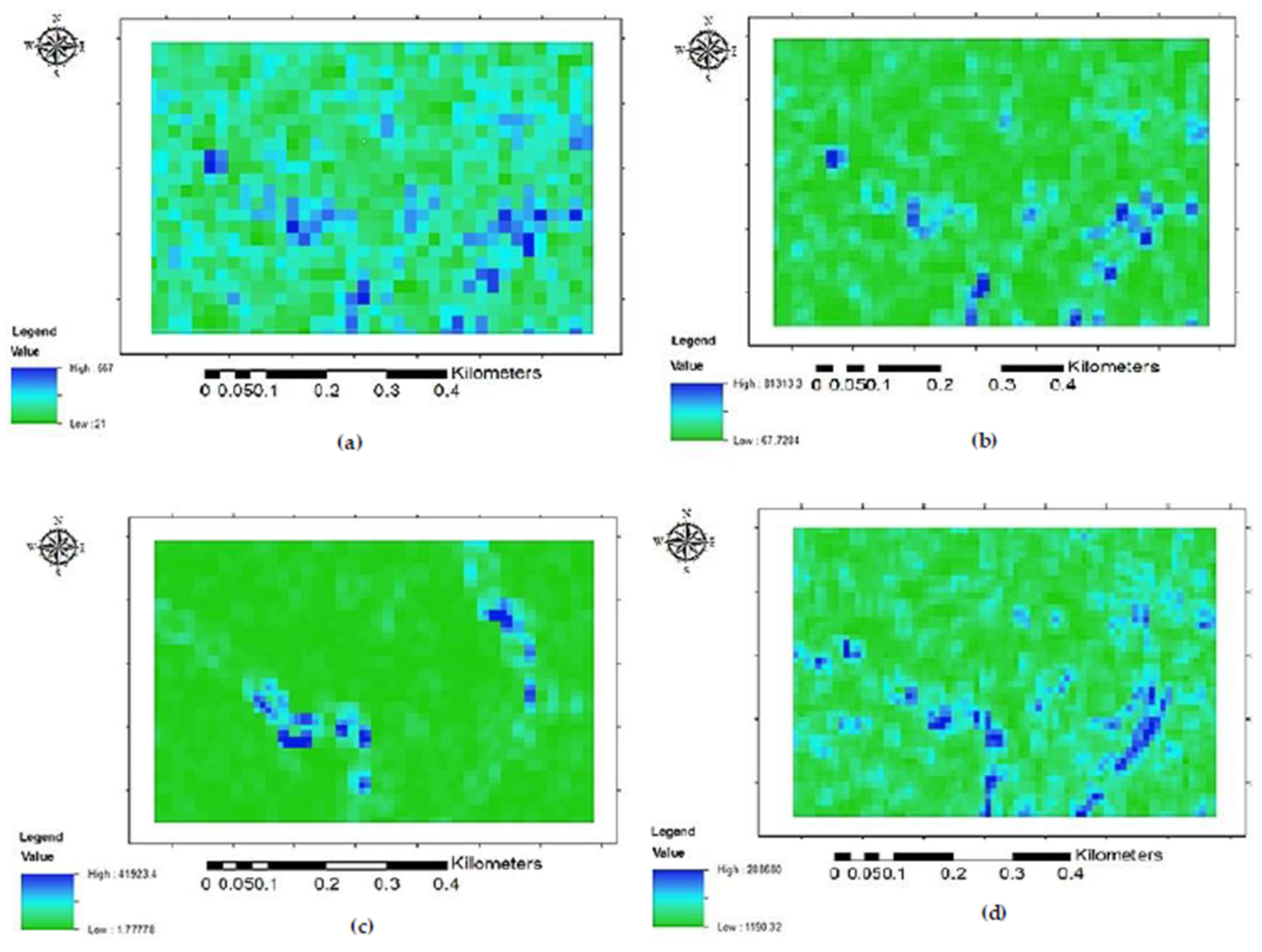
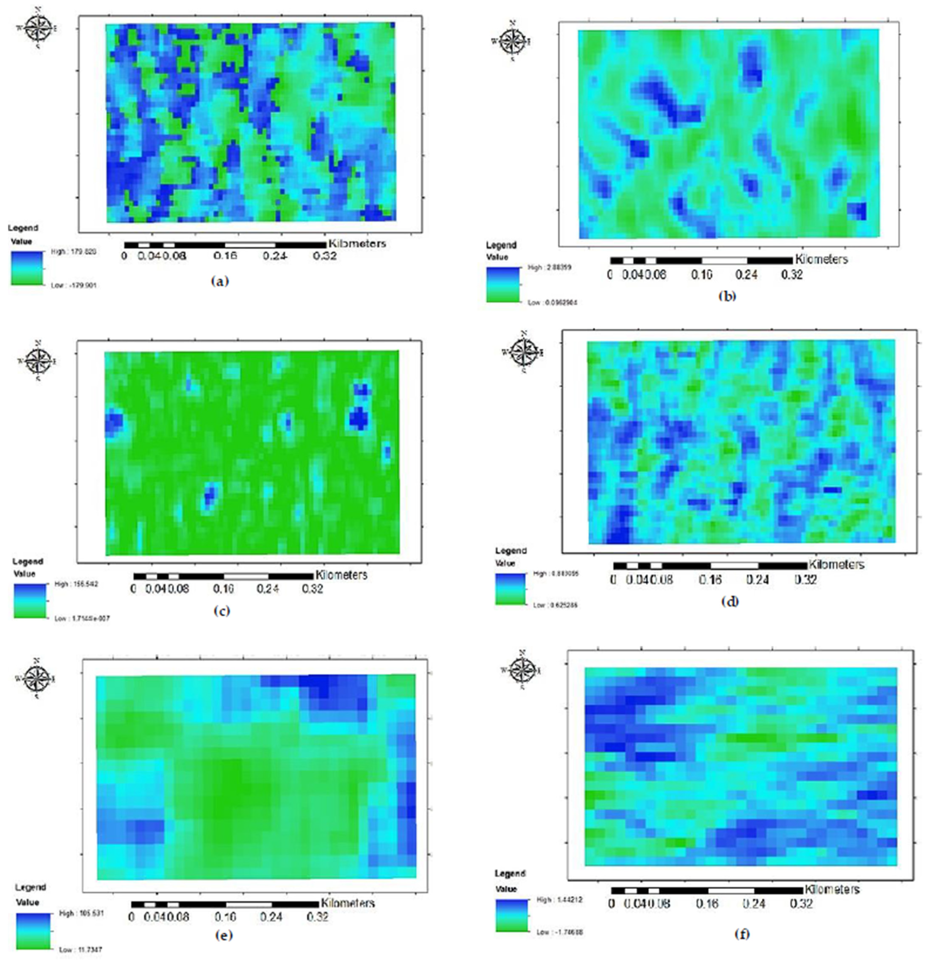
In this section, after data preprocessing and indices extraction, the AGB and carbon stock maps were determined by GA-RF method. First, the best indices of Optical and SAR Data were selected by GA algorithm, distinctly (Figure 3 and Figure 4). The quantitative result which were used R² to analyse GA-RF model of AGB.

As mentioned, in this study, the total number of field data plots is 39. About 70% and 30% of them were selected as model train and test data, respectively. The measured AGB plots and the measured indices of the data were also considered as response variables and independent variables, respectively. In this model, among 27 bootstrap samples, 100 decision trees (ntrees) were achieved the best result for AGB modeling by optical data and 300 decision trees for AGB modelling by SAR data (Figure 5). Optimization of the number of trees variable is calculated by minimizing the RMSE using test data. The final output (AGB) was the average output of decision trees.

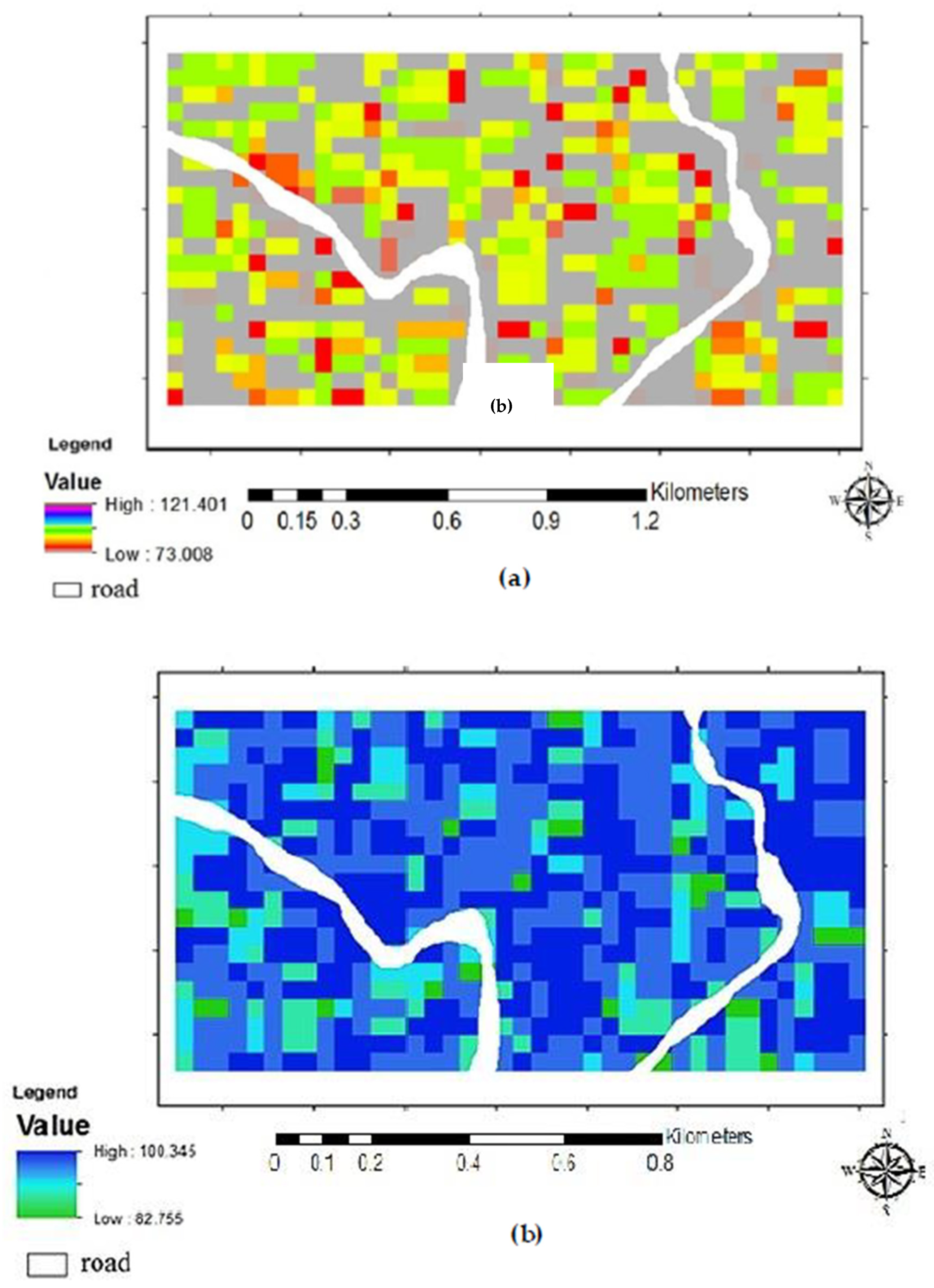
Figure 6 shows the results of the proposed method which are the biomass predictions obtained from the RF model of the best performance using the optical and SAR data. The road area was masked out.

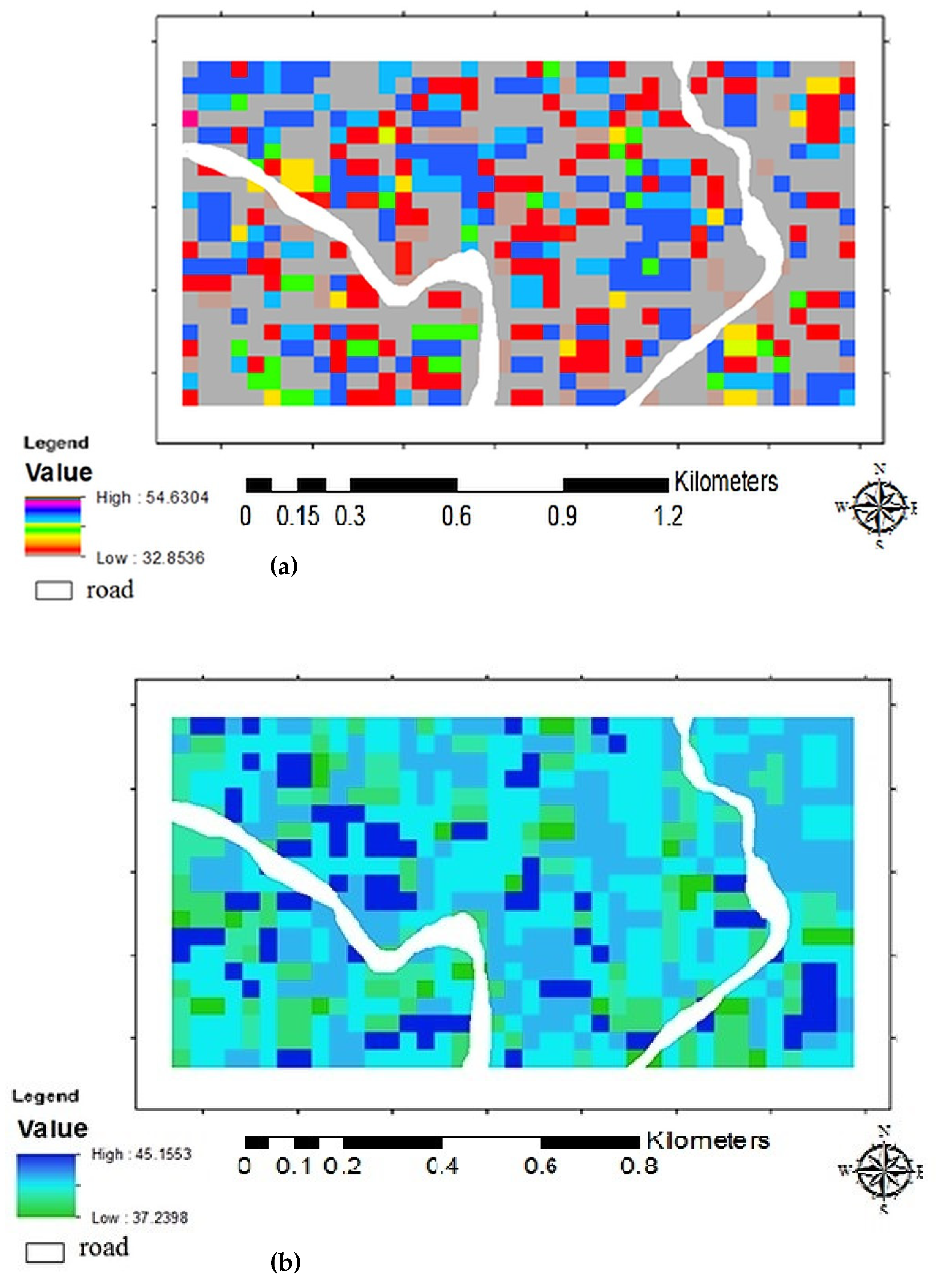
The AGB map is converted to carbon by the scaling factor. We use carbon fraction of dry matter conversion factor of 0.47 (Figure 7) [60].

Figure 8 compares the predicted AGB by the GA-RF model and the AGB field measurements. The results show significant accuracies which illustrate the result of AGB estimation of combination of Sentinel-1 and ALOSPALSAR data (R² = 70%) is better than the result of Sentinel-2 data (R² = 62%).

4. Conclusions

Accurate biomass assessment is essential in order to manage the forest and understand its role as a carbon source. In this study, we assessed the ability of combination of Sentinel-1 and ALOSPALSAR data, and Sentinel-2 data for mapping aboveground biomass (AGB) in a part of Hyrcanian forest of northern Iran. Vegetation indices, tasseled cap, texture parameters and principal component analysis (PCA) variables of Sentinel-2 data, and Polarimetric decompositions, texture characteristics and backscatter coefficients of Sentinel-1 and ALOSPALSAR data were extracted and used as input to GA-RF model. We reached the following conclusions from this study:

(1)

Due to the lack of access to all areas and high cost and time consuming by ground method, these problems can be overcame by using remote sensing method.

(2)

The combination of Sentinel-1 and ALOSPALSAR data illustrated better performance in estimating AGB compared to sentinel-2 data.

(3)

GA-RF Model is beneficial and fast to achieve high accuracy in AGB prediction.

(4)

The use of feature selection method (GA) to reduce the number of predictor features improved the performance of the RF model.

(5)

Effectiveness of texture and decomposition features on AGB calculation.

References

1. Luyssaert, S.; Schulze, E.-D.; Börner, A.; Knohl, A.; Hessenmöller, D.; Law, B.E.; Ciais, P.; Grace, J. Old-growth forests as global carbon sinks. Nature 2008, 455, 213–215. [Google Scholar] [CrossRef] [PubMed]
2. Lu, D. The potential and challenge of remote sensing-based biomass estimation. Int. J. Remote Sens. 2006, 27, 1297–1328. [Google Scholar] [CrossRef]
3. Lu, D. Aboveground biomass estimation using Landsat TM data in the Brazilian Amazon. Int. J. Remote Sens. 2005, 26, 2509–2525. [Google Scholar] [CrossRef]
4. Foody, G.M.; Boyd, D.S.; Cutler, M.E. Predictive relations of tropical forest biomass from Landsat TM data and their transferability between regions. Remote Sens. Environ. 2003, 85, 463–474. [Google Scholar] [CrossRef]
5. TSITSI, B. Remote sensing of aboveground forest biomass: A review. Trop. Ecol. 2016, 57, 125–132. [Google Scholar]
6. Sinha, S.; Jeganathan, C.; Sharma, L.K.; Nathawat, M.S. A review of radar remote sensing for biomass estimation. Int. J. Environ. Sci. Technol. 2015, 12, 1779–1792. [Google Scholar] [CrossRef]
7. Deo, R.K. Modelling and Mapping of Above-Ground Biomass and Carbon Sequestration in the Cool Temperate Forest of North-East China; ITC Enschede: Enschede, The Netherlands, 2008. [Google Scholar]
8. Hyde, P.; Nelson, R.; Kimes, D.; Levine, E. Exploring LiDAR–RaDAR synergy—predicting aboveground biomass in a southwestern ponderosa pine forest using LiDAR, SAR and InSAR. Remote Sens. Environ. 2007, 106, 28–38. [Google Scholar] [CrossRef]
9. Fassnacht, F.E.; Hartig, F.; Latifi, H.; Berger, C.; Hernández, J.; Corvalán, P.; Koch, B. Importance of sample size, data type and prediction method for remote sensing-based estimations of aboveground forest biomass. Remote Sens. Environ. 2014, 154, 102–114. [Google Scholar] [CrossRef]
10. Ghasemi, N.; Sahebi, M.R.; Mohammadzadeh, A. Biomass estimation of a temperate deciduous forest using wavelet analysis. IEEE Trans. Geosci. Remote Sens. 2012, 51, 765–776. [Google Scholar] [CrossRef]
11. Caicoya, A.T.; Kugler, F.; Papathanassiou, K.; Biber, P.; Pretzsch, H. Biomass estimation as a function of vertical forest structure and forest height-Potential and limitations for Radar Remote Sensing. In Proceedings of the 8th European Conference on Synthetic Aperture Radar, Aachen, Germany, 7–10 June 2010; pp. 1–4. [Google Scholar]
12. Behera, M.; Tripathi, P.; Mishra, B.; Kumar, S.; Chitale, V.; Behera, S.K. Above-ground biomass and carbon estimates of Shorea robusta and Tectona grandis forests using QuadPOL ALOS PALSAR data. Adv. Space Res. 2016, 57, 552–561. [Google Scholar] [CrossRef]
13. West, P.W. Growing Plantation Forests; Springer: Berlin, Germany, 2006. [Google Scholar]
14. Pearson, R.L.; Miller, L.D.; Tucker, C.J. Hand-held spectral radiometer to estimate gramineous biomass. Appl. Opt. 1976, 15, 416–418. [Google Scholar] [CrossRef]
15. Li, X.; Gar-On Yeh, A.; Wang, S.; Liu, K.; Liu, X.; Qian, J.; Chen, X. Regression and analytical models for estimating mangrove wetland biomass in South China using Radarsat images. Int. J. Remote Sens. 2007, 28, 5567–5582. [Google Scholar] [CrossRef]
16. Ghasemi, N.; Sahebi, M.R.; Mohammadzadeh, A. A review on biomass estimation methods using synthetic aperture radar data. Int. J. Geomat. Geosci. 2011, 1, 776–788. [Google Scholar]
17. Treuhaft, R.N.; Law, B.E.; Asner, G.P. Forest attributes from radar interferometric structure and its fusion with optical remote sensing. BioScience 2004, 54, 561–571. [Google Scholar] [CrossRef]
18. He, Q.; Cao, C.; Chen, E.; Ling, F.; Zhang, H. Relationship between SAR and biomass derived from LiDAR in Mountain areas. In Proceedings of the 2009 2nd Asian-Pacific Conference on Synthetic Aperture Radar, Xi’an, China, 26–30 October 2009; pp. 136–139. [Google Scholar]
19. Imhoff, M.L. Radar backscatter and biomass saturation: Ramifications for global biomass inventory. IEEE Trans. Geosci. Remote Sens. 1995, 33, 511–518. [Google Scholar] [CrossRef]
20. Le Toan, T.; Beaudoin, A.; Riom, J.; Guyon, D. Relating forest biomass to SAR data. IEEE Trans. Geosci. Remote Sens. 1992, 30, 403–411. [Google Scholar] [CrossRef]
21. Cutler, M.; Boyd, D.; Foody, G.; Vetrivel, A. Estimating tropical forest biomass with a combination of SAR image texture and Landsat TM data: An assessment of predictions between regions. ISPRS J. Photogramm. Remote Sens. 2012, 70, 66–77. [Google Scholar] [CrossRef]
22. Mutanga, O.; Adam, E.; Cho, M.A. High density biomass estimation for wetland vegetation using WorldView-2 imagery and random forest regression algorithm. Int. J. Appl. Earth Obs. Geoinf. 2012, 18, 399–406. [Google Scholar] [CrossRef]
23. Laurin, G.V.; Chen, Q.; Lindsell, J.A.; Coomes, D.A.; Del Frate, F.; Guerriero, L.; Pirotti, F.; Valentini, R. Above ground biomass estimation in an African tropical forest with lidar and hyperspectral data. ISPRS J. Photogramm. Remote Sens. 2014, 89, 49–58. [Google Scholar] [CrossRef]
24. Karlson, M.; Ostwald, M.; Reese, H.; Sanou, J.; Tankoano, B.; Mattsson, E. Mapping tree canopy cover and aboveground biomass in Sudano-Sahelian woodlands using Landsat 8 and random forest. Remote Sens. 2015, 7, 10017–10041. [Google Scholar] [CrossRef]
25. Tavasoli, N.; Arefi, H.; Samiei-Esfahany, S.; Ronoud, Q. Modelling the amount of carbon stock using remote sensing in urban forest and its relationship with land use change. Int. Arch. Photogramm. Remote Sens. Spat. Inf. Sci. 2019, 42, 1051–1058. [Google Scholar] [CrossRef]
26. Nuthammachot, N.; Askar, A.; Stratoulias, D.; Wicaksono, P. Combined use of Sentinel-1 and Sentinel-2 data for improving above-ground biomass estimation. Geocarto Int. 2020, 1–11. [Google Scholar] [CrossRef]
27. Brown, S. Estimating Biomass and Biomass Change of Tropical Forests: A Primer; Food & Agriculture Org.: United Nations, 1997; Volume 134. [Google Scholar]
28. Brown, S.; Lugo, A.E. Biomass of tropical forests: A new estimate based on forest volumes. Science 1984, 223, 1290–1293. [Google Scholar] [CrossRef]
29. Tarmian, A.; Remond, R.; Faezipour, M.; Karimi, A.; Perré, P. Reaction wood drying kinetics: Tension wood in Fagus sylvatica and compression wood in Picea abies. Wood Sci. Technol. 2009, 43, 113–130. [Google Scholar] [CrossRef]
30. Drusch, M.; Del Bello, U.; Carlier, S.; Colin, O.; Fernandez, V.; Gascon, F.; Hoersch, B.; Isola, C.; Laberinti, P.; Martimort, P. Sentinel-2: ESA’s optical high-resolution mission for GMES operational services. Remote Sens. Environ. 2012, 120, 25–36. [Google Scholar] [CrossRef]
31. Sandwell, D.T.; Myer, D.; Mellors, R.; Shimada, M.; Brooks, B.; Foster, J. Accuracy and resolution of ALOS interferometry: Vector deformation maps of the Father’s Day intrusion at Kilauea. IEEE Trans. Geosci. Remote Sens. 2008, 46, 3524–3534. [Google Scholar] [CrossRef]
32. Torres, R.; Snoeij, P.; Geudtner, D.; Bibby, D.; Davidson, M.; Attema, E.; Potin, P.; Rommen, B.; Floury, N.; Brown, M. GMES Sentinel-1 mission. Remote Sens. Environ. 2012, 120, 9–24. [Google Scholar] [CrossRef]
33. Ahmed, S.M.; Eldin, F.A.E.; Tarek, A.M. Speckle noise reduction in SAR images using adaptive morphological filter. In Proceedings of the 2010 10th International Conference on Intelligent Systems Design and Applications, Cairo, Egypt, 29 November–1 December 2010; pp. 260–265. [Google Scholar]
34. Lee, J.-S. Digital image enhancement and noise filtering by use of local statistics. IEEE Trans. Pattern Anal. Mach. Intell. 1980, 165–168. [Google Scholar] [CrossRef]
35. Frost, V.S.; Stiles, J.A.; Shanmugan, K.S.; Holtzman, J.C. A model for radar images and its application to adaptive digital filtering of multiplicative noise. IEEE Trans. Pattern Anal. Mach. Intell. 1982, 157–166. [Google Scholar] [CrossRef]
36. Xue, J.; Su, B. Significant remote sensing vegetation indices: A review of developments and applications. J. Sens. 2017, 2017, 1353691. [Google Scholar] [CrossRef]
37. Jackson, R.D.; Huete, A.R. Interpreting vegetation indices. Prev. Vet. Med. 1991, 11, 185–200. [Google Scholar] [CrossRef]
38. Major, D.; Baret, F.; Guyot, G. A ratio vegetation index adjusted for soil brightness. Int. J. Remote Sens. 1990, 11, 727–740. [Google Scholar] [CrossRef]
39. Carlson, T.N.; Ripley, D.A. On the relation between NDVI, fractional vegetation cover, and leaf area index. Remote Sens. Environ. 1997, 62, 241–252. [Google Scholar] [CrossRef]
40. Nellis, M.D.; Briggs, J.M. Transformed vegetation index for measuring spatial variation in drought impacted biomass on Konza Prairie, Kansas. Trans. Kansas Acad. Sci. (1903) 1992, 95, 93–99. [Google Scholar] [CrossRef]
41. Ashburn, P. The Vegetative Index Number and Crop Identification; Lyndon B. Johnson Space Center: Houston, TX, USA, 1979. [Google Scholar]
42. Mohanaiah, P.; Sathyanarayana, P.; GuruKumar, L. Image texture feature extraction using GLCM approach. Int. J. Sci. Res. Publ. 2013, 3, 1–5. [Google Scholar]
43. Crist, E.P.; Cicone, R.C. Application of the tasseled cap concept to simulated thematic mapper data. Photogramm. Eng. Remote Sens. 1984, 50, 343–352. [Google Scholar]
44. Crist, E.P. A TM tasseled cap equivalent transformation for reflectance factor data. Remote Sens. Environ. 1985, 17, 301–306. [Google Scholar] [CrossRef]
45. Richards, J. Thematic mapping from multitemporal image data using the principal components transformation. Remote Sens. Environ. 1984, 16, 35–46. [Google Scholar] [CrossRef]
46. Mo, T.; Schmugge, T.J.; Jackson, T.J. Calculations of radar backscattering coefficient of vegetation-covered soils. Remote Sens. Environ. 1984, 15, 119–133. [Google Scholar]
47. Lee, J.; Pottier, E. Introduction to the polarimetric target decomposition concept. In Polarimetric Radar Imaging: From Basics to Applications; CRC Press: Boca Raton, FL, USA, 2009; pp. 1–422. [Google Scholar]
48. Sun, G.; Ranson, K.J. A three-dimensional radar backscatter model of forest canopies. IEEE Trans. Geosci. Remote Sens. 1995, 33, 372–382. [Google Scholar] [CrossRef]
49. Jayasri, P.; Niharika, K.; Joseph, M.; Ryali, H.U.S.; Sarma, C.R.; Kumari, E.S.; Prasad, A. Implementation of RISAT-1 hybrid polarimetric decomposition techniques and analysis using corner reflector data. J. Indian Soc. Remote Sens. 2018, 46, 1005–1012. [Google Scholar] [CrossRef]
50. Raney, R.K.; Cahill, J.T.; Patterson, G.W.; Bussey, D.B.J. The m-chi decomposition of hybrid dual-polarimetric radar data with application to lunar craters. J. Geophys. Res. Planets 2012, 117. [Google Scholar] [CrossRef]
51. Raney, R.K. M-chi decomposition of imperfect hybrid dual-polarimetric radar data. ESASP 2013, 713, 2. [Google Scholar]
52. Raney, R.K. Decomposition of hybrid-polarity SAR data. In PolIn-SAR 2007, Proceedings of the 3rd International Workshop on Science and Applications, Frascati, Italy, 22–26 January 2007; European Space Agency: Noordwijk, The Netherlands, 2007; pp. 22–26. [Google Scholar]
53. Cloude, S.R.; Goodenough, D.G.; Chen, H. Compact decomposition theory. IEEE Geosci. Remote Sens. Lett. 2011, 9, 28–32. [Google Scholar] [CrossRef]
54. Singh, G.; Venkataraman, G.; Rao, Y. The H/A/Alpha polarimetric decomposition theorem and complex wishart distribution for snow cover monitoring. In Proceedings of the IGARSS 2008—2008 IEEE International Geoscience and Remote Sensing Symposium, Boston, MA, USA, 7–11 July 2008; pp. IV-1081–IV-1084. [Google Scholar]
55. Breiman, L. Random forests. Mach. Learn. 2001, 45, 5–32. [Google Scholar] [CrossRef]
56. Pal, M. Random forest classifier for remote sensing classification. Int. J. Remote Sens. 2005, 26, 217–222. [Google Scholar] [CrossRef]
57. Mitchell, M. An Introduction to Genetic Algorithms; MIT Press: Cambridge, MA, USA, 1998. [Google Scholar]
58. Ali, E.E.E.; Elamin, E. A Proposed Genetic Algorithm Selection Method; King Saud University, College of Computer and Information Sciences: Riyadh, Saudi Arabia, 2006. [Google Scholar]
59. Oh, I.-S.; Lee, J.-S.; Moon, B.-R. Hybrid genetic algorithms for feature selection. IEEE Trans. Pattern Anal. Mach. Intell. 2004, 26, 1424–1437. [Google Scholar]
60. Bernal, B.; Murray, L.T.; Pearson, T.R. Global carbon dioxide removal rates from forest landscape restoration activities. Carbon Balance Manag. 2018, 13, 22. [Google Scholar] [CrossRef]
Figure 1. Location of the study area. The blue figure on the upper right, Mazandaran Province and the lower right Landsat image show the exact location of the area.
Environsciproc 05 00013 g001
Figure 2. Flowchart of steps used for AGB and carbon stock estimation in this study.
Environsciproc 05 00013 g002
Figure 3. The best selected features of the Optical data for biomass estimation by GA: (a) texture (Data range variable) of band 6, (b) texture (variance variable) of band 6, (c) texture (variance variable) of band 5, (d) texture (variance variable) of band 8.
Environsciproc 05 00013 g003
Figure 4. The best selected features of the SAR data for biomass estimation by GA: (a) m- δ decomposition (Delta variable) of Sentinel-1, (b) Compact decomposition (Compact RSOV variable) of Sentinel-1, (c) Compact decomposition (Compact pd variable) of Sentinel-1, (d) H/A/Alpha decomposition (P1 variable) of Sentinel-1, (e) texture (Homogeneity variable) of Sentinel-1, (f) Eigen vector decomposition (Entropy variable) of ALOSPALSAR.
Environsciproc 05 00013 g004
Figure 5. The RMSE variation based on ntree: (a) modelling by optical data, (b) modelling by SAR data.
Environsciproc 05 00013 g005
Figure 6. Above ground biomass derived from GA-RF: (a) AGB by optical data, (b) AGB by SAR data.
Environsciproc 05 00013 g006
Figure 7. Carbon stock derived from GA-RF: (a) carbon stock map by optical data, (b) carbon stock map by SAR data.
Environsciproc 05 00013 g007
Figure 8. Comparisons between the field AGB and predicted AGB derived from Optical and SAR data: (a) modelling by Optical data, (b) modelling by SAR data.
Environsciproc 05 00013 g008