Next Article in Journal
FORTLS: An R Package for Processing TLS Data and Estimating Stand Variables in Forest Inventories
Previous Article in Journal
Nutrient Sustainability in Swiss Wood Extraction
 
 
Please note that, as of 4 December 2024, Environmental Sciences Proceedings has been renamed to Environmental and Earth Sciences Proceedings and is now published here.
Proceeding Paper

An External Agribusiness Risk Analysis Using KBDI: A Case of Veldfires in the Northern Territory of Australia †

by
Toyi Maniki Diphagwe
1,
Bernard Moeketsi Hlalele
2,* and
Dibuseng Priscilla Mpakathi
1
1
Disaster Management Training and Education Centre for Africa (DiMTEC), Faculty of Natural and Agricultural Sciences, University of the Free State, Bloemfontein 9300, South Africa
2
Department of Business Support, Faculty of Management Sciences, Central University of Technology, Free State, Bloemfontein 9300, South Africa
*
Author to whom correspondence should be addressed.
Presented at the 1st International Electronic Conference on Forests—Forests for a Better Future: Sustainability, Innovation, Interdisciplinarity, 15–30 November 2020; Available online: https://iecf2020.sciforum.net.
Environ. Sci. Proc. 2021, 3(1), 37; https://doi.org/10.3390/IECF2020-08065
Published: 13 November 2020

Abstract

:
The 2019/20 Australian bushfires burned over 46 million acres of land, killed 34 people and left 3500 individuals homeless. Majority of deaths and buildings destroyed were in New South Wales, while the Northern Territory accounted for approximately 1/3 of the burned area. Many of the buildings that were lost were farm buildings, adding to the challenge of agricultural recovery that is already complex because of ash-covered farmland accompanied by historic levels of drought. The current research therefore aimed at characterising veldfire risk in the study area using Keetch-Byram Drought Index (KBDI). A 39-year-long time series data was obtained from an online NASA database. Both homogeneity and stationarity tests were deployed using a non-parametric Pettitt’s and Dicky-Fuller tests respectively for data quality checks. Major results revealed a non-significant two-tailed Mann Kendall trend test with a p-value = 0.789 > 0.05 significance level. A suitable probability distribution was fitted to the annual KBDI time series where both Kolmogorov-Smirnov and Chi-square tests revealed Gamma (1) as a suitably fitted probability distribution. Return level computation from the Gamma (1) distribution using XLSTAT computer software resulted in a cumulative 40-year return period of moderate to high fire risk potential. With this low probability and 40-year-long return level, the study found the area less prone to fire risks detrimental to animal and crop production. More agribusiness investments can safely be executed in the Northern Territory without high risk aversion.

1. Introduction

The bulk of the world’s veldfires are man-made. Human-caused fires result from camping fires left burning, debris burning, equipment usage and malfunctions, cigarettes negligently discarded and deliberate incendiary actions. Other veldfires are caused by nature such as lightning. There are two forms of lightning—cold flash and hot flash. Cold lightning is a return stroke with intense but relatively short-lived electrical current. Hot lightning has lower voltage currents, but these occur over a longer period. Fires are typically ignited by hot lightning bolts that are exceptionally long-lasting [1]. These veldfires destroy around 14 million hectares of fire-prone forests globally each year, a level of destruction and depletion equivalent to that of destructive deforestation and agricultural conversion [2]. At the same time, many forest habitats that are adapted to fire are becoming heat starved. Human beings, including government agencies responsible for forest resource management, are altering natural fire regimes around the globe without taking into consideration the long-term implications. Moore (2003) [3] in his article believes policymakers and the public are best positioned to respond to repeated short-term problems than to concentrate attention on long-term, sustainable solutions. Resources need to be redirected to promote work that enhances knowledge of fire causes, recognises existing management practices that encourage hazardous fires and fosters management structures that emulate natural fire regimes or make the most of the well-known fuel usage.
Sometimes dealing with fires is interpreted as fighting fires or adding fire-fighting power, but that method does not work. The communications sent to politicians and communities also provide a very clear picture of a complicated situation, not all the following issues regarding fires are actually real: (i) Extreme weather triggers veldfires, (ii) All veldfires are toxic, (iii) Every fire should be stopped and extinguished, and (iv) Veldfires are the most concerned with regular occurrences as they happen [1].
Explanations that are unnecessarily simplistic about veldfire theories continue to allow lawmakers to take the view that fire suppression is the primary remedy for dangerous veldfires. To date, insufficient focus has been devoted to tackling underlying causes and attempting to prevent a spiralling downward of repeated flames and degradation in burnt locations.

2. International Case Studies

The map in Figure 1 shows principal causes, veldfires form and size. This map is an approximation provided that fire statistics are limited for certain regions. There is a distinction between natural or human-induced causes (in the story, N or H), and ground fire forms and crown fire. Low frequency means a period of fire over 200 years, med frequency over 20 to 200 years, and a high frequency over less than 20 years [4].
Regarding ecosystems based on fire, the National Research Council (2011) in their study found that eco-regions worldwide rely on or are affected by heavy fire. Veldfires in these regions are so important to the protection of human flora and fauna, as are rain and sunlight. Typical fire ecosystems include the taiga, African grasslands, South Asian rainy season and dry forests, Australia’s eucalyptus forests, California’s coniferous forests, the Mediterranean region and all pine forests from taiga to subtropics. With fire, all these habitats formed [5]. Fire frequency and intensity depend on natural variables such as climate, a form of vegetation, lightning strike, accumulated biomass or land. Burns retain the characteristic ecosystem structure and composition that has evolved with fire. All these habitats are not burning in the same way though. For example, low-intensity ground fires are common and required in many forests, grasslands, savannahs and wetlands to preserve an open landscape with a multitude of grasses and shrubs [6]. Certain forest and bushland habitats depend on uncommon, but extreme, fires that rejuvenate people. What sets all fire-dependent ecosystems apart, however, is the resilience of the plant and animal populations and capacity to recover, provided that the fire stays within the limits imposed by factors that are natural. Fire prevention can deliver far-reaching environmental and environmental benefits and socially unwanted ecosystem changes. For example, full fire prevention has caused the traditional grass scenery of some parts of the Southwest USA offering both wildlife and cattle food turn into thick pine woods with little grass growth, providing fuel for fires that are extremely dangerous and damaging [7].

3. Veldfires and Changing Climate

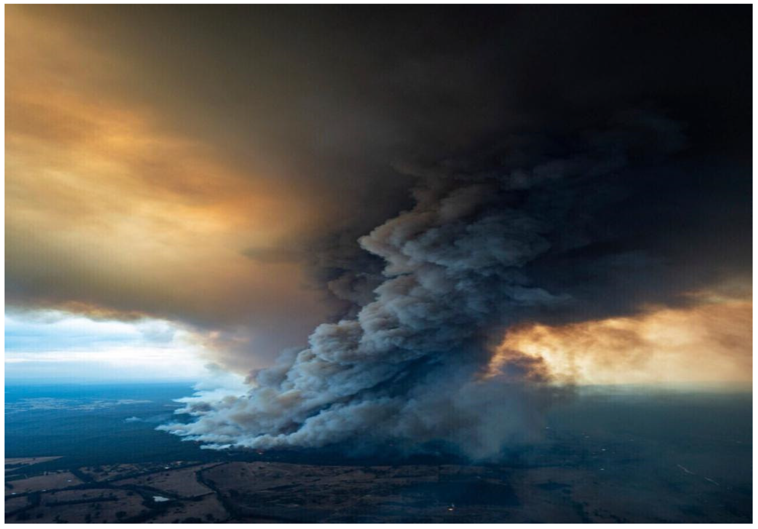
Veldfires contribute by causing the release of greenhouse gases in relation to climate change, significantly (Figure 2). The warmer climate contributes to forests becoming dryer and damaged, which makes them more vulnerable to flames. A rise in the number and intensity of fires generates a positive feedback loop [8]. The study by WWF (2017) [7] found savannah and veldfires release 1.6 to 4.1 billion tons of carbon per annum atmospheric dioxide; additionally, approximately 38 million t of methane (CH4; 1 t CH4 = 21 t CO2) and 21 million t of carbon dioxide Nitrogen oxides (NOx) and sulfur dioxide (SO2) of 3.5 million tons are produced every year. Attributed to 15 percent of global GHG emissions are shot trees. Most are caused by the clearing of fires in tropical rainforests and the subsequent land conversion. Veldfires are responsible for 33 percent of the world carbon monoxide and 10 percent of methane emissions as well as more than 86 percent of soot. Several studies suggest that climate change will increase the number of hot and dry days with elevated fire risks, will extend fire season and will increase electrical storm frequency. This will increase the incidence of veldfires and affect the forest region.

4. Australian Fires

Veldfires make up an integral part of the Australian climate. Natural ecosystems have evolved with fire, and the landscape and its biodiversity have been changed by both historical and recent fires. Most of Australia’s indigenous plants are fire resistant and highly flammable, while other organisms rely on fire for regeneration [9]. Fire has long been used by indigenous Australians as a method for land management, and it remains to be used to clear land for agricultural purposes and to protect property from extreme, uncontrolled fires. Largely, veldfires have caused casualties and significant damage to land. Although natural veldfires cannot be prevented, their effects can be minimised through the implementation of mitigation measures and the possible effects on the most vulnerable areas [10].
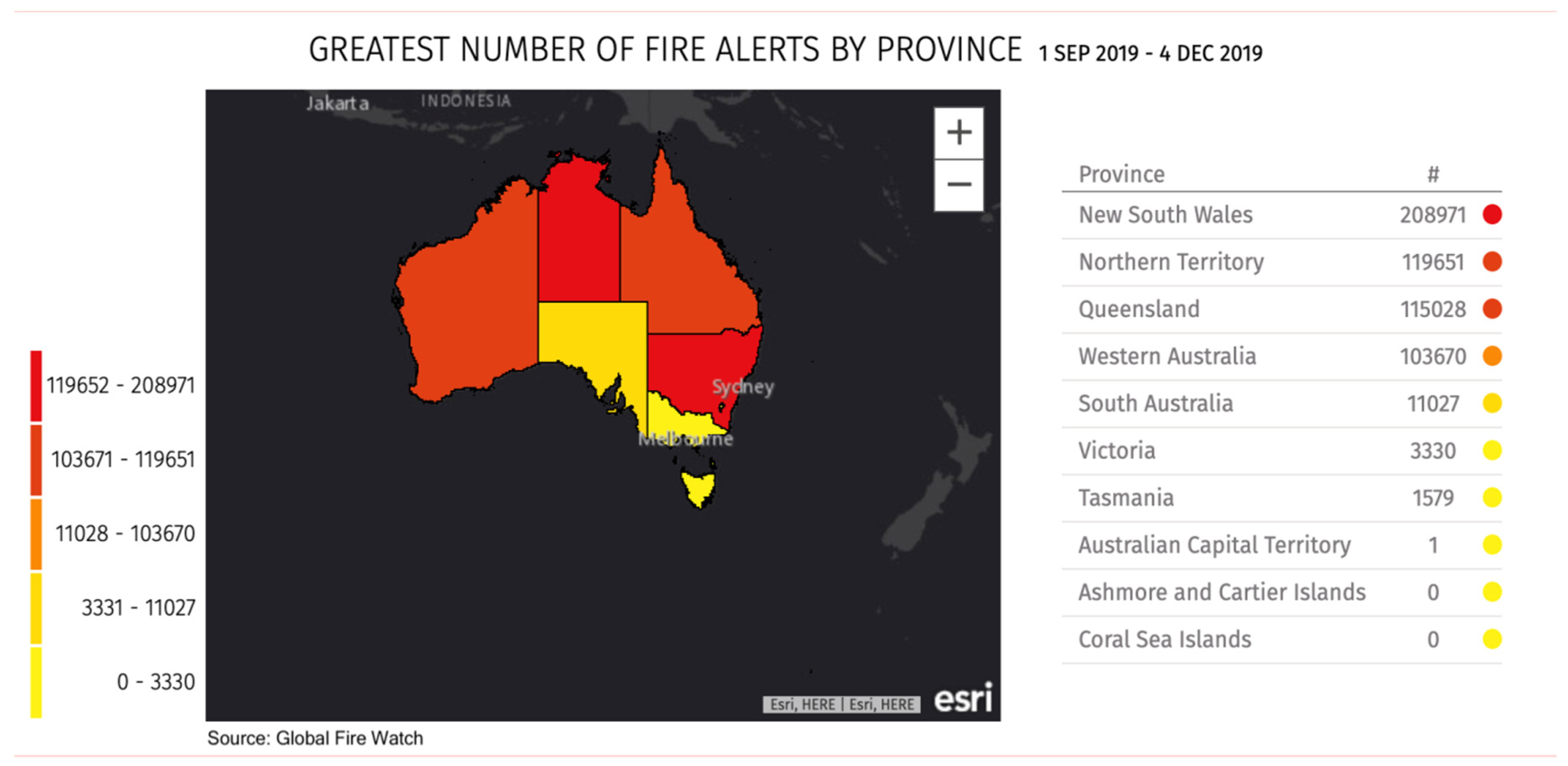
The Government of Australia in 2013 reported that the temperature is hot, dry and drought prone. At any time of year, certain parts of Australia are vulnerable to veldfires as shown in Figure 3. The widely varying fire seasons are reflected in the continent’s varied weather conditions. The time of danger to much of the South of Australia is summer and autumn [11]. The biggest threat usually occurs during spring and early summer for New South Wales and southern Queensland. The Northern Territory experiences the bulk of its fires in winter and spring. Grassland fires frequently occur after good rainfall periods, leading to overgrowth that dries out during extreme heat [12]. If such extreme fire weather is experienced in the vicinity of populated areas, the big loss is probable. With regards to the total area burnt, the main fires are in the Northern Territory and northern parts of Western Australia and Queensland. Most life losses and financial harm occur in the outskirts of cities where usually residences are next to combustible vegetation [13].

5. The Correlation between Climate and Veldfires

Climate plays a significant part in the creation, development and death of a veldfire. Drought contributes to absolutely disastrous veldfire situations, and winds aid a wildfire progress—climate can drive the fire to travel faster and consume more ground. It can also make the battle against fire a lot harder. The atmosphere contains three ingredients which can cause veldfires: temperature, wind speed and precipitation [14].

6. Temperatures

Temperature affects the sparking of veldfires as mentioned above because heat is one of the three components of the fire triangle. On the ground, the rocks, leaves and underbrush receive direct heat from the sun that heats and dries up possible fuels. NASA, (2019) [15] released a report stating that warmer temperatures allow more rapid ignition and burning of fuels, adding to the pace at which a veldfire spreads. For that reason, when temperatures are at their hottest, veldfires appear to rage in the afternoon. The heat from the sun is transmitted by radiation into the earth. This heat warms the earth’s surface, and the near-surface atmosphere is warmed up by the heat emanating from the air. That is the reason the surface temperature is hotter than the surface of the earth. Typically, such temperature drops by an altitude of about 3.5 degrees per 304.8 m. This decline is known as adiabatic lapse rate [15].

7. Precipitation

Wind possibly has the greatest effect on veldfire’s behaviour. It also represents the most unpredictable factor. For the prescribed firefighter burners, the wind is important because of three characteristics it has on veldfire behaviour:
  • Oxygen supply for the incineration process
  • Reduction of fuel moisture through enhanced evaporation
  • Exerting pressure to physically transfer the fire and heat generated closer to the fuel in the fire path through radiation like pitching burning embers, firebrands in some cases [16].
Wind may be the most persistent problem. It can change acceleration, course, or it can become very ragged. Fire propagation rate and intensity are affected by wind. High winds will easily trigger the head of a fire to travel forward. It may cause the fire to crown the peak of the trees and leap barriers that normally stop a fire [17].

8. Methods and Materials

The research approach is a plan and process consisting of measures to be used in the study, from general conclusions to detailed data collection, analysis and interpretation methods. However, the method to be used is based on the topic of analysis to be addressed [18]. There are three types of research approaches: qualitative approach, quantitative method and mixed method. The qualitative approach places a heavy emphasis on methods of data collection or generation. As Creswell and Clarke observed in 2011, a researcher is given a chance to promote more rigorous study when both qualitative and quantitative are applied in a mixed system. In order to forecast the probability and intensity of veldfires and classify them using the Keetchy-Byram drought index in the Northern Territory, Australia, the present study used a quantitative method to achieve a full statistical overview.

9. Data Quality Control

The primary aim of data integrity security is to help detect data errors in the process of data processing, whether or not done purposely (deliberate forgery) (systematic or unintended error) [19]. Quality assurance and quality control are described as two techniques that can protect the integrity of data and ensure that the results are correct and reliable in scientific terms [20].

10. Outliers in Datasets

In a randomly chosen sample, an outlier is the product of a group of individuals, which is an abnormal range from other values. This explanation places it in a way that the analyst determines what can be considered abnormal [21]. Before it is possible to pick anomalous observations, regular observations need to be noted. There are two types of outliers: multivariable and univariate. When viewing a value distribution, univariate outliers may be found within a single space of a function [22]. Multivariate outliers can be found in an n-dimensional space (of n-features), which can be very difficult for the human mind to look at distribution in n-dimensional spaces, so we can build a network to do it for us. Outliers can occur in many ways and hide in some measurements in the collection, generation, analysis and processing of data. Novelties are not the outcomes produced in error [23]. The detection of outliers is of critical importance in almost every quantitative discipline, (i.e., economy, cybersecurity) [24]. The quality of data is as important in the quantitative method as the quality of a forecast. To detect outliers in a dataset, this study will use SPSS (Social Science Statistical Package), which is a series of interconnected software programs in a single package. The central goal of this program is to evaluate social science-based empirical evidence. It is used between various data variables to analyse, transform and create a pattern of characteristics.

11. Stationarity Test in Time Series

A stationary time series is one whose statistical properties, such as mean, variance, autocorrelation, etc., are all constant over time [25]. Statistical prediction models are based on the premise that the time series in mathematical transformations (i.e., “stationarised”) will be approximately stationary. Predicting a stationary sequence is fairly straightforward: you practically conclude that in the future its statistical characteristics would be the same as they were in the past [26]. In order to obtain predictions for the original sequence, the predictions for the stationary sequence can then be “untransformed” by removing any previously used mathematical transformations (the software normally takes care of the specifics.) Therefore, finding the sequence of changes required to stationarise a time series also provides helpful clues in the search for an effective forecasting model [27].
Reliable sample statistics, such as means, variances and correlations with other variables, are a justification for attempting to stationarise a time series. If the series is stationary, these statistics are only useful as descriptors of potential behaviour [27]. For example, if the series increases continuously over time, the mean and variance of the sample will rise with the sample size, and in future periods, they will often underestimate the mean and variance. If a series’ mean and variance are not well-defined, then its correlations with other variables are not either. For this reason, one should be careful to try to extrapolate regression models fitted to non-stationary data [28]. The Dicky-Fuller test is used for this study to determine the existence of the unit root in the series, helping us to understand whether or not the series is stationary.

12. Homogeneity Test in Time Series

Before any statistical technique is applied to it, the assessment of whether a data set is homogeneous is always important. It draws a single population from homogeneous data [29]. In other words, all external processes that may affect the data potentially must remain constant for the entire time of the survey. Inhomogeneities are caused by a period in which the statistical properties of the observations are influenced by artificial modifications [30]. Such changes can be abrupt or gradual, depending on the nature of the disruption. It is almost difficult to obtain completely homogeneous data realistically, since the data would always be impacted by inevitable shifts in the environment around the observation station [30].
It is common practice to apply statistical methods to climate measurements, including software development, to check the homogeneity of time series. Relative homogeneity tests examining series relating to allegedly homogeneous stations are preferred to absolute tests measuring a single position only [31]. These comparative studies, which can be carried out in close proximity to sufficiently correlated stations, are better able to detect inhomogeneities from actual variations in temperature but are not able to cope with simultaneous shifts in both stations’ experimental routines [29]. Absolute tests are required in the event of low space station density. The tool used to determine the homogeneity of time series is the Pettitt test, a non-parametric test adapted from the Mann-Whitney rank-based test that allows the definition of the point at which the transition takes place in a time series [32].

Data Analysis

Analysis involves splitting the information into subjects, trends, patterns and relationships that can be handled. The aim of data analysis is to evaluate the different components of one’s data by analysing the relationship between values, structures or variables and to see if there are any trends or patterns that can be detected or isolated or to identify themes in interpretation [33]. Descriptive statistics require summarising and organising the details in order to make it easier to understand. Descriptive statistics strive to explain the results, unlike inferential statistics, but do not try to bring inferences from the sample to the entire population. Here, we normally describe the details in a report. This generally implies that unlike inferential statistics, descriptive statistics are not constructed on the basis of probability theory [34]. Descriptive temperature and rainfall statistics to explore main trend indicators (mean, median) and measurements of variability (range, standard deviation, variance) will be analysed in this report.

13. Mann Kendall’s Test and Keetchy-Byram Drought Index

The Mann-Kendall test is performed to determine whether in its upward or downward trend, a time series is monotonic. It does not allow for the normal or linear distribution of the data. No auto-relationship needs it [35]. This study will assess whether the input datasets have any important patterns.
The drought index was established in 1968 by Keetchy and Byram for fire control purposes [36]. The Keetchy-Byram drought index has been the most commonly used in monitoring and prediction of veldfires, largely due to its simple implementation compared to other indices that typically need more meteorological data and complex calculations [37]. The KBDI, which conceptually defines the soil moisture deficit, is used as an intermediate quantity evaluating the drought fuel load supply and as a stand-alone index for assessing fire hazard. The index was designed to function in a wide range of climatic and precipitation situations in forest or wildland areas [38]. Variations of KBDI and its application to operate in veldfires have been analysed. Descriptive statistics were used for quantitative analysis, and findings were described by pie charts, frequency distributions and bar graphs. The KBDI starting values are assumed to be significantly proportional to the percentage of effects on soil moisture expressed as a share of field energy. When calculating KBDI, the following (Equation (1)) is used Keetch, (1968):
dQ =   [ 800     Q ]   [ 0.968   exp   ( 0.0486 T   0.830 ]   dr 1 + 10.88 exp ( 0.04441 R ) × 10 3
where:
  • dQ = Drought factor, the unit is 0.01 in
  • Q = Moisture deficiency, the unit is 0.01 in
  • T = Daily max temperature, the unit is ⁰F
  • R = Mean annual precipitation, the unit is in
  • dr = Time increment, the unit is 1 day
The KBDI is trying to indicate the level of rainfall needed to restore the soil to the maximum potential of the field. This is a sealed 0- to 800-unit structure which reflects a 0- to 8-inch water moisture regime through the layer of soil. At 8 inches of water, the KBDI assumes saturation. Zero is the degree of no moisture shortage, and the maximum possible drought is 800. The index number indicates the amount of net rainfall needed to lower the index to zero, or saturation, at any point along the scale. KBDI inputs are latitude at the weather station, mean annual precipitation, average dry bulb temperature and the last 24 h of rainfall. Drought relief happens only in situations where rainfall reaches 0.20 inches (called net rainfall). The statistical measures include rising the drought index by the net amount of rain and increasing the drought index by a factor of drought [39]. Below is the table of KBDI interpretation (Table 1).

14. Results and Discussion

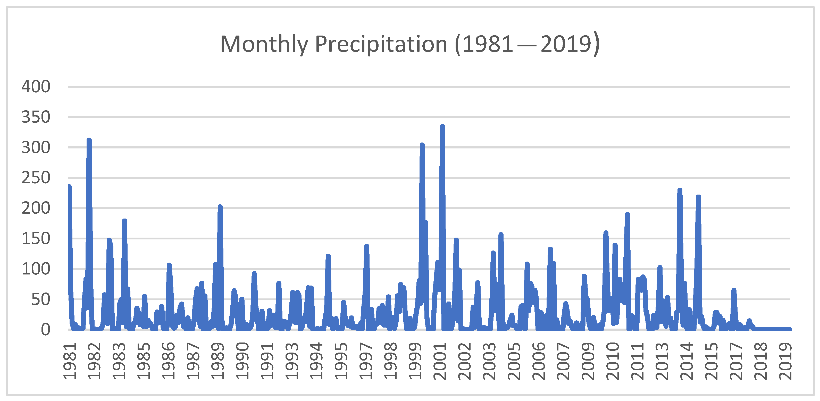
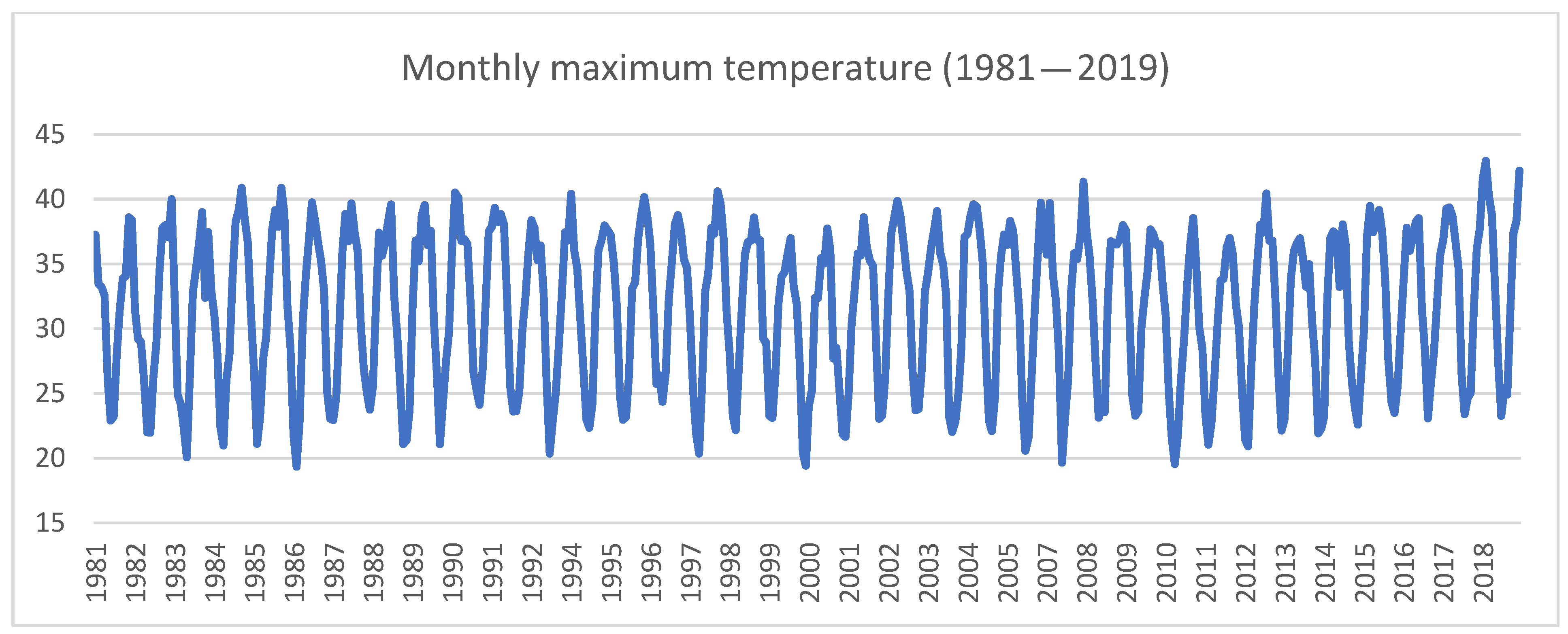
Figure 4 and Figure 5 depict the plots of monthly maximum temperature and precipitation from 1981 to 2019. These are the two input parameters used in the computation of KBDI. Virtually, it can be seen that precipitation dataset had several outliers while maximum temperature had uniform values over the years. The outliers had to be removed prior to further analysis of data in order to bring about reliable final results.
Table 2 and Figure 6 below show descriptive statistics and box and whisker plot for both precipitation and maximum temperature respectively. From Figure 6, it can be seen that the precipitation dataset contained outliers while there was none in the maximum temperature as depicted by the box-plots.
Table 3, Table 4 and Table 5 show that results of tests done prior to the final analysis of the datasets. Table 3 shows a non-parametric homogeneity test for both precipitation and maximum temperature where the two datasets proved to be homogenous and ready to be used in further analysis. Stationarity test was also conducted through the use of Dickey-Fuller test and Phillip-Perron Tests. The results show that the dataset was stationary, hence there is no need for any transformations as proven by a non-significant one-tailed p-value of 0.675 of Dickey-Fuller test and significant one tailed p-value of 0.003 as shown in Table 4. Table 5 showed non-significant results of Pettitt’s test, implying homogenous datasets.
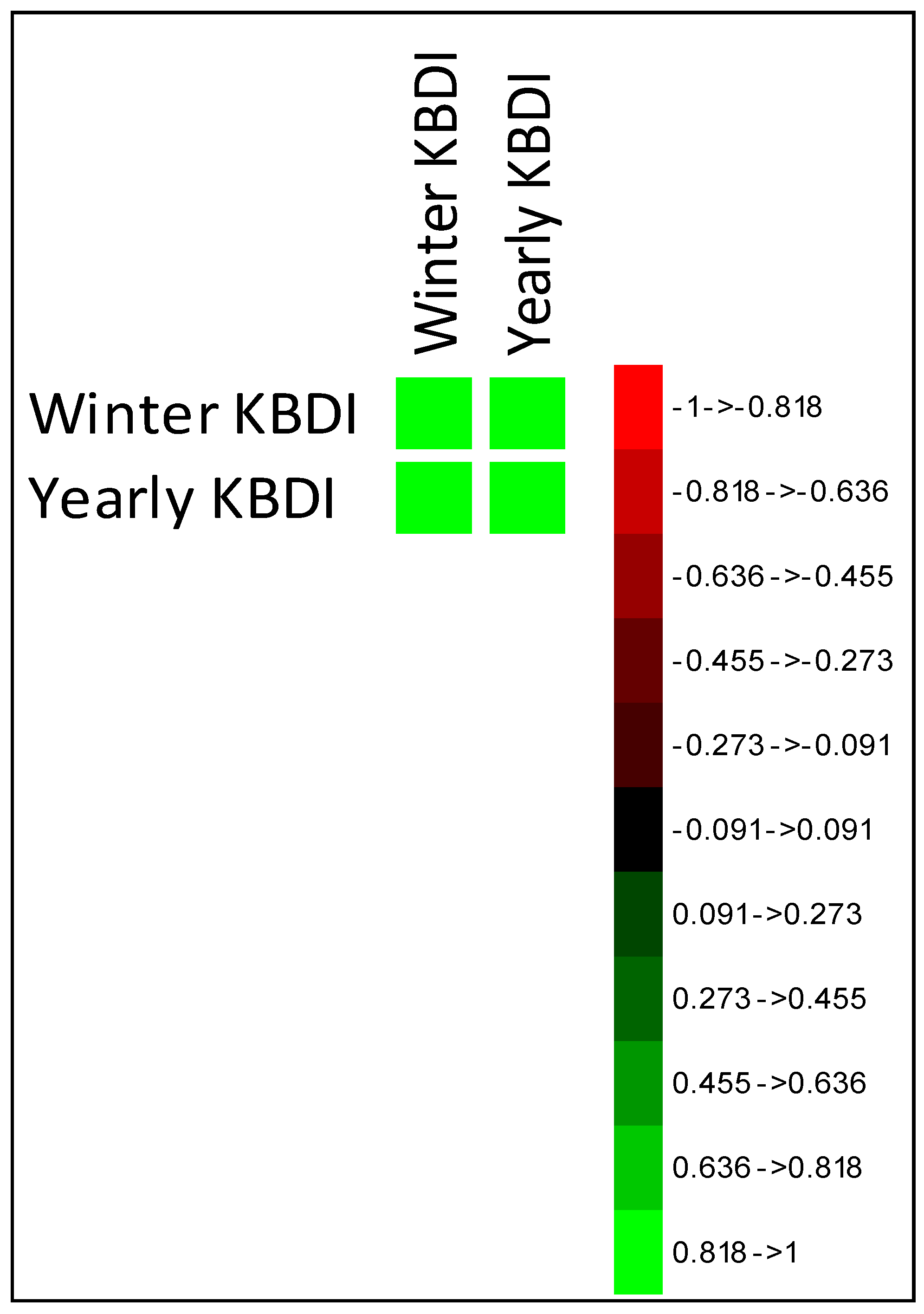
According to Table 6, the two computed temporal scales, winter and yearly KBDI, had relatively the same variabilities with similar variance of approximately 16. These two selected scales were similar across all descriptive statistic values, hence a non-parametric test needed to prove their relationship as shown in Table 7. The correlation test result was very significant with p-value < 0.0001. The results were further illustrated in Figure 7 to clearly indicate how closely correlated these two time scales are. This phenomenon clearly indicates that most fires in the study area occur in winter, which happens to be the key season in Australia for veldfires.
Having determined the key season for Australian fires and its relationship to annual fires, it was therefore necessary to determine if any monotonic trends were present in the KBDI time series. Table 8 shows a non-parametric Mann Kendall trend test which showed no trend in the series with a non-significant p-value of 0.789. In order to determine the return periods of veldfires in the area, since there was no trend pattern detected, the KBDI time series was fitted to a statistically suitable probability distribution aided by XLSTAT computer software. A suitably fitted distribution was Gamma (1) with parameters shown in Table 9, Table 10, Table 11 and Table 12. Two fitting criterion tests, Kolmogorov-Smirnov and Chi-square, were used to judge the fitted distribution, where both pointed at Gamma (1) being the best fitted probability distribution. This distribution was used in the computation of the return periods of the study area veldfires.

15. Conclusion and Recommendations

In conclusion, the 2019/20 Australian bushfires burned over 46 million acres of land, killed 34 people and left 3500 individuals homeless. Majority of deaths and buildings destroyed were in New South Wales, while the Northern Territory accounted for approximately 1/3 of the burned area. Many of the buildings that were lost were farm buildings, adding to the challenge of agricultural recovery that is already complex because of ash-covered farmland accompanied by historic levels of drought. The current therefore aimed at characterising veldfire risk in the study area using Keetch-Byram Drought Index (KBDI). A 39-year-long time series data was obtained from an online NASA database. Both homogeneity and stationarity tests were deployed using a non-parametric Pettitt’s and Dicky-Fuller tests respectively for data quality checks. Major results revealed a non-significant two-tailed Mann Kendall trend test with a p-value = 0.789 > 0.05 significance level. A suitable probability distribution was fitted to the annual KBDI time series where both Kolmogorov-Smirnov and Chi-square tests revealed Gamma (1) as a suitably fitted probability distribution. Return level computation from the Gamma (1) distribution using XLSTAT computer software resulted in a cumulative 40-year (1/39 = 2.5%) return period of moderate to high fire risk potential. With this low probability and 40-year-long return level, the study found the area less prone to fire risks detrimental to animal and crop production. More agribusiness investments can safely be executed in the Northern Territory without high risk aversion.

Data Availability Statement

Data presented is not inappropriately selected, manipulated, enhanced, or fabricated. No persons were involved in this study for data collection, and plagiarism was avoided by the full quoting of sources cited in the report. Data used on this study was accessed from: NASA. Power Access Viewer [online] on https://power.larc.nasa.gov/data-access-viewer/.

References

  1. WFMI. Fire Reporting—Annual Dataset Archive. 2018. Available online: https://wfmi.nifc.gov/fire_reporting/annual_dataset_archive/index.html (accessed on 20 June 2020).
  2. Butler, A. Consequences of Deforestation; Mongabay: Menlo Park, CA, USA, 2019. [Google Scholar]
  3. Moore, P.; Hardesty, J.; Kelleher, S.; Maginnis, S.; Myers, R. Forests and Wildfires: Fixing the Future by Avoiding The Past. 2003. Available online: http://www.fao.org/3/xii/0829-b3.htm (accessed on 20 May 2020).
  4. Bowman, D.M.J.S.; Balch, J.; Artaxo, P.; Bond, W.J.; Cochrane, M.A.; D’Antonio, C.M.; DeFries, R.; Johnston, F.H.; Keeley, J.E.; Krawchuk, M.A.; et al. The human dimension of fire regimes on Earth. J. Biogeogr. 2011, 38, 2223–2236. [Google Scholar] [CrossRef] [PubMed]
  5. Butler, A. The Year Rainforests Burned; Mongabay News and Inspiration from Nature’s Frontline, 2012. [Google Scholar]
  6. FAO. Public Meeting on Policies Affecting Forest Fires; FAO: Rome, Italy, 1998. [Google Scholar]
  7. WWF. Forests Ablaze: Causes and Effects of Global Forest Fires. 2017. Available online: https://mobil.wwf.de/fileadmin/fm-wwf/Publikationen-PDF/WWF-Study-Forests-Ablaze.pdf (accessed on 7 May 2020).
  8. USGCRP. Climate Change in the United States: The Third National Climate Assessmemnt; U.S. Global Change Research Program: Washington, DC, USA, 2014.
  9. Munroe, T.; Taylor, R. 4 Things to Know about Australia’s Wildfires and Their Impacts on Forests. 2020. Available online: https://www.wri.org/blog/2020/01/4-things-know-about-australia-s-wildfires-and-their-impacts-forests (accessed on 6 May 2020).
  10. Bowman, D.M.J.S. The impact of Aboriginal landscape burning on the Australian biota. New Psychol. 2008, 140, 385–410. [Google Scholar]
  11. Geoscience Australia. Bushfire. 2013. Available online: https://www.ga.gov.au/scientific-topics/community-safety/bushfire (accessed on 25 June 2020).
  12. Guadian. Australia Bushfires Factcheck: Are This Year’s Fires Unprecedented? 2019. Available online: https://www.theguardian.com/australia-news/2019/nov/22/australia-bushfires-factcheck-are-this-years-fires-unprecedented (accessed on 6 May 2020).
  13. Thornton, R. Bushfires 1: Understanding Bushfires; Australian Academy of Science: Sydney, Australia, 2016. [Google Scholar]
  14. WMO. Drought and Heat Exacerbate Wildfires; World Meteorologial Organisation: Geneva, Switzerland, 2018. [Google Scholar]
  15. NASA. Correlation between Temperature and Radiation. 2019. Available online: http://www.ces.fau.edu/nasa/module-2/correlation-between-temperature-and-radiation.php (accessed on 7 May 2020).
  16. The Burn. Weather Elements that Affect Fire Behavior. 2019. Available online: https://www.auburn.edu/academic/forestry_wildlife/fire/weather_elements.htm (accessed on 30 April 2020).
  17. Bushfire Foundation. Fire Behaviour. 2020. Available online: https://www.thebushfirefoundation.org/how-fire-behaves/ (accessed on 13 June 2020).
  18. Creswell, J. Research Design: Qualitative, Quantitative, and Mixed Methods Approaches; s.l. SAGE: Thousand Oaks, CA, USA, 2013. [Google Scholar]
  19. Whitney, C.; Lind, B.K.; Wahl, P.W. Quality assurance and quality control in longitudinal studies. J. Epidermiol. Rev. 1998, 20, 71–80. [Google Scholar] [CrossRef] [PubMed]
  20. Most, M.M.; Craddick, S.; Crawford, S.; Redican, S.; Rhodes, D.; Rukenbrod, F.; Laws, R. Dietary quality assurance processes of the DASH-Sodium controlled diet study. J. Am. Diet. Assoc. 2003, 103, 1339–1346. [Google Scholar] [CrossRef]
  21. Tuckey, J. Exploratory Data Analysi; Addison-Wesley: Menlo Park, London, UK, 1977; pp. 43–44. [Google Scholar]
  22. Quesada, A. Outlier Detection; KD Nuggets: Madrid, Spain, 2017. [Google Scholar]
  23. Santoyo, S. A Brief Overview of Outlier Detection Techniques; Towards Data Science: Eindhoven, 2017. [Google Scholar]
  24. Cousineau, D.; Chartier, S. Outliers detection and treatmen: A review. Int. J. Psychol. Res. 2010, 3, 58–67. [Google Scholar] [CrossRef]
  25. Cardinali, A.; Nason, G.P. Costationary of locally stationary time series. J. Time Ser. Econ. 2010, 2. [Google Scholar] [CrossRef]
  26. Palachy, S. Stationarity in Time Series Analysis; Towards Data Science: Israel, 2019. [Google Scholar]
  27. Dahlhaus, R. Locally stationary process. In Handbooks of Statistics; Cornell University: New York, 2012; Volume 30, pp. 351–413. [Google Scholar]
  28. Myers, D. To be or not be … stationary? That is the question. Math. Geol. 1989, 21, 347–362. [Google Scholar] [CrossRef]
  29. Yozgatlingil, C.; Yazici, C. Comparison of homogeinity test for temperature using a simulation study. Int. J. Climatol. 2016, 36, 62–81. [Google Scholar] [CrossRef]
  30. Yasizi, C.; Yozgatligil, C.; Batmaz, I. A Similation Study on the Performance of Homogeneity Tests Applied in Meteriological Studies. In Proceedings of the ICAMC: International Conference on Applied and Computational Mathematics, Ankara, Turkey, 3–6 October 2012. [Google Scholar]
  31. Karl, T.; Williams, C.N., Jr.; Young, P.J.; Wendland, W.M. A model to estimate the time of observation bias association with monthly mean maximum, minimum and mean temperatures for the United States. J. Appl. Mater. 1986, 18, 145–160. [Google Scholar]
  32. Pettitt, A. A non-parametric approach to change pooint problem. J. R. Stat. Soc. Ser. C Appl. Stat. 1979, 28, 126–139. [Google Scholar]
  33. Mouton, J. How to Succeed in Your Master’s and Doctoral Studies, 24th ed.; Van Schaik: Pretoria, South Africa, 2019. [Google Scholar]
  34. Kaur, P.; Stoltzfus, J.; Yellapu, V. Descriptive Statistics. Int. J. Acad. Med. 2018, 4, 60–63. [Google Scholar] [CrossRef]
  35. Kendall, M. The Advance Theory of Statistics, 2nd ed.; Charles: London, UK, 1967. [Google Scholar]
  36. Keetch, J. A Drought Index for Forest Fire Control; USAD Forest Services: North Carolina, 1968.
  37. Antonio, D.; Del Campo, A.; Tarcísio Fernandes, J.G.; Antonio Molina, J. Development of a Keetchy and Byram—Based drought index sensitive to forest management in Mediterranean conditions. Agric. For. Meteorol. 2015, 205, 40–50. [Google Scholar]
  38. Johnson, M. Spatial Mapping of KBDI for the Southeast of United States; America Meteorological Society: Nevada, USA, 2001. [Google Scholar]
  39. WFAS. Wild Fire Assessment System. 2020. Available online: wfsa.net (accessed on 28 April 2020).
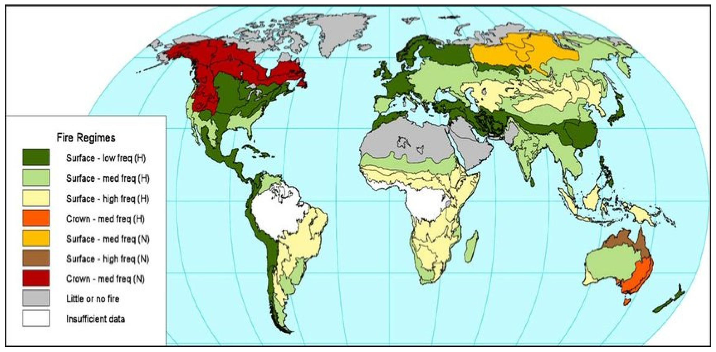
Figure 1. World Fire Regime map. Sourced: www.fao.org/forestry/fo/fra/index.jsp.
Environsciproc 03 00037 g001
Figure 2. Picture depicting how smoke affects the climate. Photo was taken by Colleen WalshHarvard, 2020.
Environsciproc 03 00037 g002
Figure 3. Fire alerts by states in Australia. Sourced: Global fire watch.
Environsciproc 03 00037 g003
Figure 4. Monthly precipitation (1981—2019): Northern Territory of Australia.
Environsciproc 03 00037 g004
Figure 5. Monthly maximum temperature (1981—2019): Northern Territory of Australia.
Environsciproc 03 00037 g005
Figure 6. Monthly precipitation and maximum temperature (1981–2019): Northern Territory of Australia.
Environsciproc 03 00037 g006
Figure 7. Winter and yearly KBDI Image of the correlation matrix.
Environsciproc 03 00037 g007
Table 1. Keetch-Byram Drought Index (KBDI) interpretation.
KBDIClassFire Potential
0–2001Soil moisture and fuel moisture of great quality are high and do not contribute much to the strength of fire. Typical of dormant spring season following winter rainfall.
200–4002Typical of late spring, season to rise early. Lower layers of litter and duff dry, and begin to add to the strength of fire.
400–6003Early fall, which is common for late summer. Lower litter and duff levels actively contribute to the strength of flames and burn actively.
600–8004More severe drought is also associated with the occurrence of intensified veldfires. With extreme downwind spotting, intense-burning fires could be anticipated. Live fuels may also be expected to actively burn at these levels.
Table 2. Descriptive statistics (Quantitative data): Precipitation and maximum temperature.
StatisticPrecipitationMaximum Temperature
Nbr. of observations468468
Minimum0.0000.000
Maximum100.000100.000
Range100.000100.000
1st Quartile0.21928.886
Median2.39457.179
3rd Quartile10.19474.439
Mean7.89152.227
Variance (n-1)178.274642.760
Standard deviation (n-1)13.35225.353
Variation coefficient (n-1)1.6920.485
Table 3. Pettitt’s test: Precipitation and Maximum Temperature.
PrecipitationMax Temp
K4125.00012,025.000
t20152015
p-value (Two-tailed)0.6750.741
alpha0.050.05
Table 4. Time series stationarity test.
ParameterDickey-Fuller TestPhillips-Perron Test
Tau (Observed value)−13.663−1.515
Tau (Critical value)−3.398−1.942
p-value (one-tailed)0.6480.003
alpha0.050.05
Table 5. Homogeneity test: Pettitt’s test (Maximum Temperature).
K4125.00012,025.000
t20152015
p-value (Two-tailed)0.6750.741
alpha0.050.05
Table 6. Keetch-Byram Drought Index (KBDI). Descriptive statistics (Quantitative data).
StatisticWinter KBDIYearly KBDI
Nbr. of observations3939
Minimum0.0000.000
Maximum100.000100.000
Range100.000100.000
1st Quartile0.0030.001
Median0.0260.007
3rd Quartile0.0310.008
Mean3.2033.185
Variance (n − 1)260.545260.991
Standard deviation (n − 1)16.14116.155
Variation coefficient (n − 1)5.0405.072
Table 7. Correction test between winter and yearly KBDI: Spearman.
VariablesWinter KBDIYearly KBDI
Winter KBDI0<0.0001
Yearly KBDI<0.00010
Table 8. Mann-Kendall trend test/Two-tailed test (Yearly KBDI).
Kendall’s Tau−0.032
S−23.000
Var(S)6784.333
p-value (Two-tailed)0.789
Alpha0.05
Table 9. Estimated parameter (Gamma (1)).
ParameterValueStandard Error
k0.2790.043
Table 10. Log-likelihood statistics.
Log-Likelihood(LL)−969.891
BIC(LL)1943.445
AIC(LL)1941.781
Table 11. Kolmogorov-Smirnov test.
D0.324
p-value (Two-tailed)0.000
Alpha0.05
Table 12. Chi-square test.
Chi-Square (Observed Value)0.103
Chi-square (Critical value)
p-value (Two-tailed)<0.0001
Alpha0.05
Publisher’s Note: MDPI stays neutral with regard to jurisdictional claims in published maps and institutional affiliations.