Proceeding Paper

An Analysis of Ionospheric Conditions during Intense Geomagnetic Storms (Dst ≤ −100 nt) in the Period 2011–2018 †

by
Charbeth Lopez Urias
1,*,
Karan Nayak
1,
Guadalupe Esteban Vazquez Becerra
1 and
Rebeca Lopez Montes
2
1
Faculty of Earth and Space Sciences, Autonomous University of Sinaloa, Culiacán 80040, Mexico
2
Department of Applied Geophysics, Center for Scientific Research and Higher Education of Ensenada, Tijuana 22860, Mexico
*
Author to whom correspondence should be addressed.
Presented at the 6th International Electronic Conference on Atmospheric Sciences, 15–30 October 2023; Available online: https://ecas2023.sciforum.net/.
Environ. Sci. Proc. 2023, 27(1), 18; https://doi.org/10.3390/ecas2023-16344
Published: 27 November 2023
(This article belongs to the Proceedings of The 6th International Electronic Conference on Atmospheric Sciences)

Abstract

:
The layer of the Earth’s atmosphere known as the ionosphere presents a significant obstacle to global satellite navigation systems (GNSS) due to its ability to introduce errors. To address this challenge, various navigation systems have introduced new signals designed to minimize the errors caused by the ionosphere. These signals not only aid in error reduction but also facilitate the examination of electron content behavior. This study focuses on the analysis of vTEC plots obtained from RINEX data collected at the INEG station in Aguascalientes, Mexico, from 2011 to 2018, with a particular emphasis on highly intense geomagnetic storms characterized by values below −100 nT. Our analysis of these plots employed the Probability Density Function (PDF), which allows for the graphical representation of data distribution. This distribution is then examined in conjunction with the station’s Total Electron Content (TEC) values and the Dst index during the corresponding geomagnetic storm events. The findings establish the correlation between each of these parameters during such events.
Keywords:
GNSS; ionosphere; TEC; PDF

1. Introduction

The ionosphere’s influence on the signals of Global Navigation Satellite Systems (GNSS) has long been recognized as a primary source of errors in satellite-based positioning. However, its significance extends far beyond mere technical challenges, encompassing a pivotal role in global communications and a susceptibility to various factors, most notably solar events [1]. Within the framework of GNSS, the dual-frequency capabilities of systems like GPS play a crucial role in characterizing ionospheric behavior. This capability allows for the assessment of ionospheric effects and facilitates the determination of Total Electron Content (TEC), providing insights into electron density variations along the satellite–receiver path. Furthermore, the Sun, as a celestial powerhouse, exerts a profound influence on the ionosphere [1,2,3]. Solar phenomena such as coronal mass ejections, solar flares, and solar energetic particle events can instigate disruptive consequences, affecting telecommunications, radiocommunications, and satellite-based systems [4,5]. The objectives of this study were to investigate ionospheric behavior during intense geomagnetic storms and to explore its interplay with solar and seasonal cycles. Drawing from historical contexts, in this paper, we delve into the evolution of ionospheric research, its ionization processes, and the pivotal role that GNSS have played in advancing our comprehension of this enigmatic layer of Earth’s atmosphere [1,6]. Furthermore, a hypothesis is formulated, suggesting that geomagnetic storms can induce significant ionospheric disturbances, and a statistical tool, the Probability Density Function (PDF), is proposed for event classification and analysis. By addressing these key aspects, this manuscript contributes to a deeper understanding of the ionosphere’s multifaceted role and its implications for both navigation and global communication systems. With a focus on 22 intense geomagnetic storms occurring between 2011 and 2018, characterized by Dst index values of less than −100 nT, this study aims to unravel the ionospheric behavior during these disruptive events. By investigating the interplay between geomagnetic storms, solar cycles, and seasonal variations, this manuscript seeks to advance our understanding of the ionosphere’s multifaceted role, ultimately benefiting global navigation and communication systems.

2. Data Used and Methodology

In this study, data for the Dst index were acquired from the website of the Center for Data Analysis for Geomagnetism and Space Magnetism at the University of Kyoto. A Python code was developed to plot the data. The criteria for obtaining the Dst index data focused on geomagnetic storms with Dst index values less than −100 nT. After identifying the events, RINEX data for the selected station were downloaded, and the Total Electron Content (TEC) was calculated using GPSTEC software version 2.9.5. These TEC data were used to create vTEC plots. Subsequently, Probability Density Functions (PDFs) were applied to the ionospheric plots using MATLAB R2017b. Our analysis involved categorizing ionospheric storms as positive or negative, examining maximum TEC values, minimum Dst index values, solar and seasonal cycles, and local time.
For TEC calculation, the dual-frequency nature of the GPS system was utilized to assess ionospheric effects. The Total Electron Content (TEC) can be calculated using phase measurements, where TEC = 9.52(R2 − R1), or pseudorange measurements, where TEC = 9.52(R2 − R1) [7]. The phase-based TEC calculation provides precise temporal variations, while the pseudorange method offers absolute values. The GPS observations were adjusted for satellite and receiver delays, multipath effects, and receiver noise [8]. Additionally, the PDF was used to analyze the probability distribution of variable values. The PDF identifies regions of higher and lower probabilities for a continuous random variable [9,10]. The PDF for a distribution can be obtained by differentiating the cumulative distribution function (CDF) [10]. The PDFs for transformed variables were computed using the Jacobian matrix. Moments and statistics were also considered to derive asymptotic PDFs.

3. Results

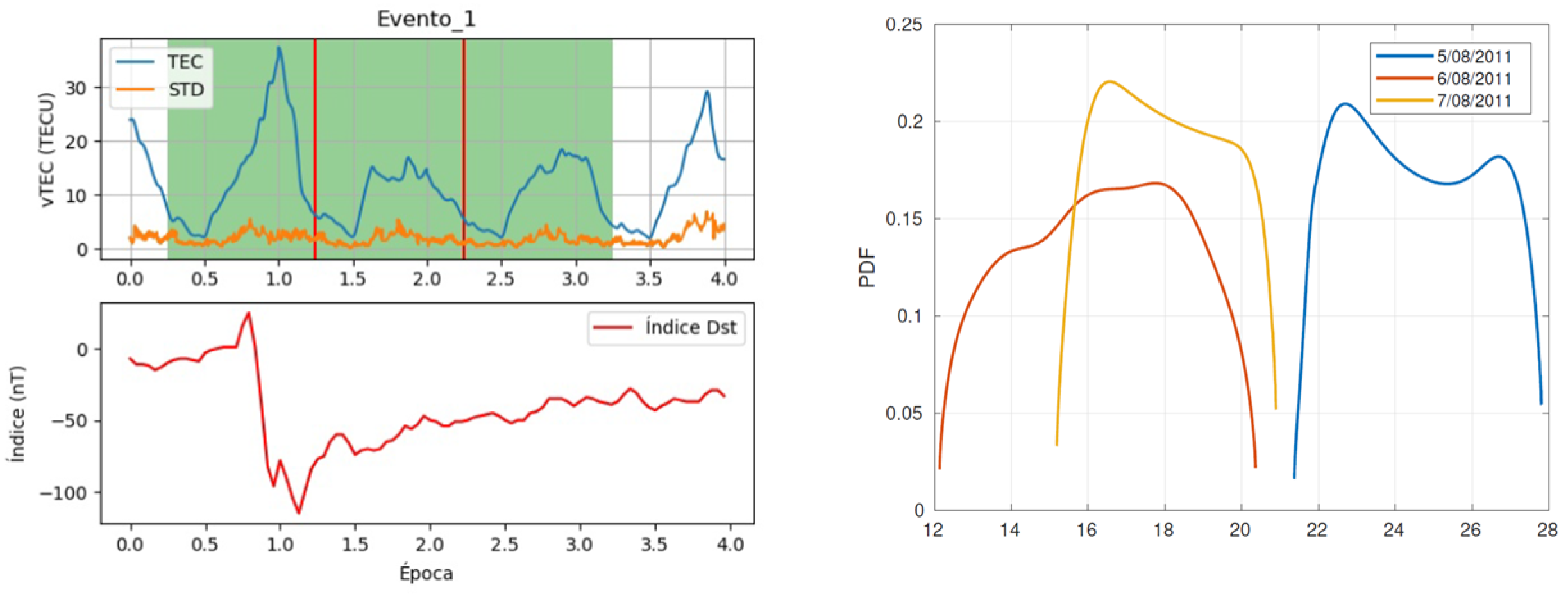
3.1. Event 1 (6 August 2011)

On 6 August 2011, a geomagnetic storm with a Dst index of −115 nT occurred (considered intense). Negative ionospheric disturbances were observed during this storm, with a vTEC value of 35.34 TECU being recorded the day before, while during and after the storm, values of 16.91 and 18.42 TECU were reached, respectively. The vTEC and Dst index graph for this event is shown in Figure 1. The Probability Density Function (PDF) results for this event, displayed in Figure 1, demonstrate the range of vTEC values before, during, and after the event.

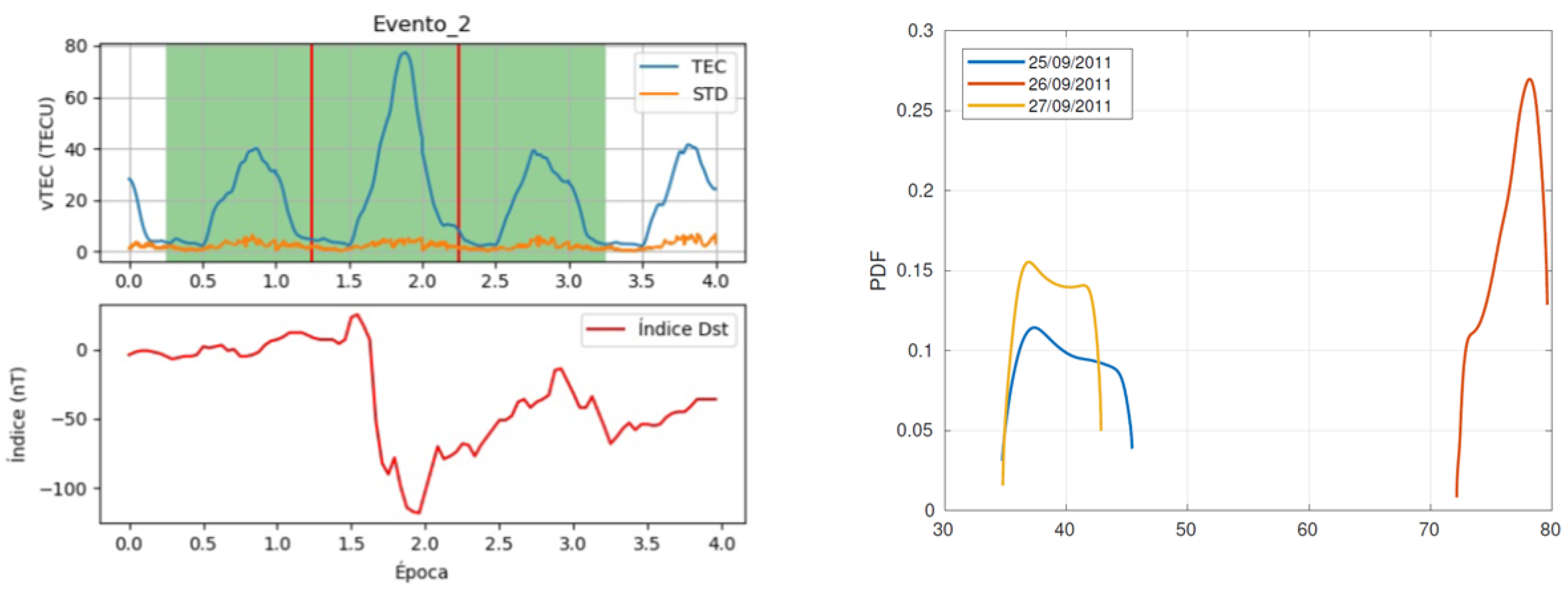
3.2. Event 2 (26 September 2011)

The 26 September 2011 storms caused significant ionospheric alterations, with vTEC values reaching 77.32 TECU during the storm. Before the storm, the TEC value was 40.01 TECU, and they quickly recovered to 39.29 TECU after the storm, indicating a positive ionospheric storm. Although intense, this geomagnetic storm had a Dst index of −118 nT, suggesting it was not as perturbing as other events from the same solar cycle. Figure 2 illustrates the variations in vTEC and the geomagnetic index for this event. The PDF results in Figure 2 show uniform alterations in vTEC throughout the study region during the event.

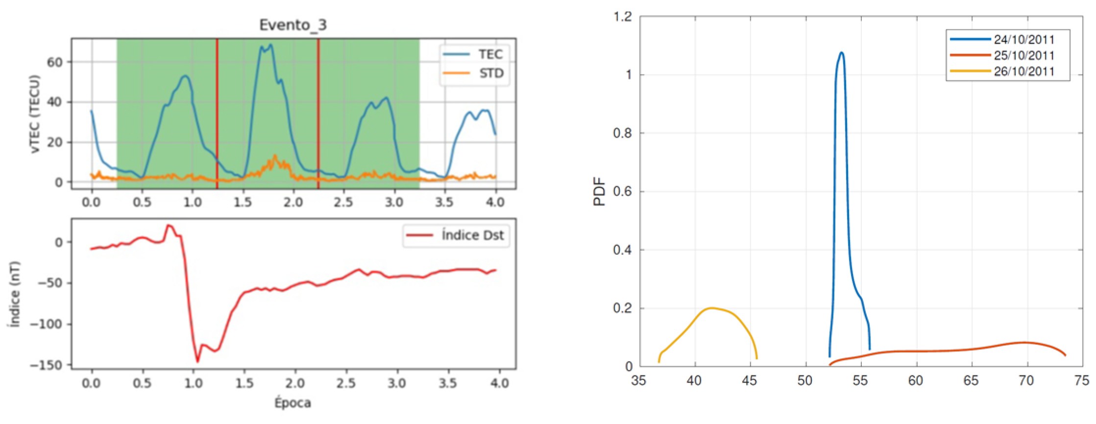
3.3. Event 3 (25 October 2011)

On 25 October 2011, the strongest geomagnetic storm of 2011 occurred, with a Dst index reaching −134 nT and peaking at 6:00 UT. This storm led to positive ionospheric disturbances, as evident in Figure 3, along with an increase in standard deviation. Interestingly, the largest data dispersion is not observable at the peak of the storm but rather during other times. Figure 3 shows the PDF results for this event, highlighting the vTEC increase in the study region, with a small area preserving its previous values due to their uniformity the day before the storm.

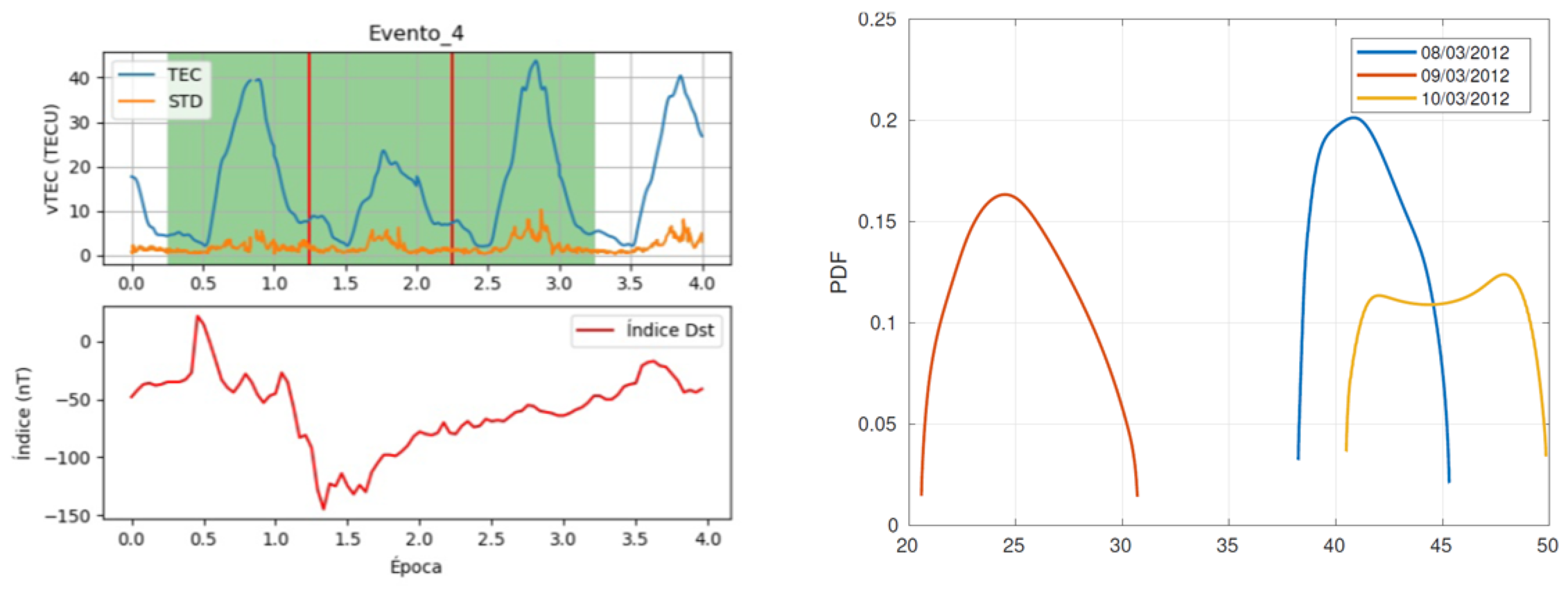
3.4. Event 4 (9 March 2012)

The event on 9 March 2012 had an intensity of −145 nT, peaking at 9:00 UT. Despite ranking as the fifth most intense storm of Solar Cycle 24, it resulted in negative ionospheric disturbances, as shown in Figure 4. The PDF results in Figure 4 reveal changes in the vTEC range during the event. Although the ionosphere experienced higher variations in the region after the event, its recovery was rapid, as the event only negatively impacted the ionosphere for one day.
The subsequent occurrences are detailed in the table beneath, Table 1, along with their respective effects on the ionosphere.
Across various geomagnetic events, notable fluctuations in the Total Electron Content (TEC) and the Dst index were observed. Event 5, which occurred on 24 April 2012, had a Dst Index of −120 nT and negatively impacted the ionosphere, with TEC changing from 59.29 TECU before the storm to 50.32 TECU during and 56.03 TECU after. Event 6, which occurred on 15 July 2012, had a unique ionospheric behavior with slow recovery, and Event 7, which occurred on 1 October 2012, negatively affected the ionosphere during the day, reaching 33.38 TECU. Event 8, which occurred on 9 October 2012, had varying impacts on the ionosphere over three days. Event 9, which occurred on 14 November 2012, was positively influenced, with TEC increasing from 37.70 TECU before the storm to 54.94 TECU during. Furthermore, Event 10, which occurred on 17 March 2013, had a positive impact, with TEC rising from 43.80 TECU before the storm to 80.93 TECU during. Event 11, which occurred on 1 June 2013, had a unique pattern with a negative impact, causing the ionosphere’s recovery to be slow. These events highlight the varying effects of geomagnetic storms on the ionosphere’s Total Electron Content. Event 12, which took place on 29 June 2013, had a significant negative impact on TEC, which reached its lowest point (−102 nT) at 7:00 h UTC with a nighttime peak. This storm hindered ionospheric recovery, leading to relatively low TEC values during the day, with a minor nighttime increase being noted at the end of 28 June 2013. Event 13 (19 February 2014) coincided with heightened solar activity but displayed a positive TEC response, peaking at 65.00 TECU during the storm and reverting to 50.08 TECU afterward. Event 14 (17 March 2015), the most intense of Solar Cycle 24 with a Dst of −222 nT, caused notable TEC variations. The TEC decreased during the day and rose in the evening, impacting the ionosphere even post-storm. Event 15 (23 June 2015), the second most intense of the cycle, brought about a severe negative ionospheric effect, with TEC values declining from 55.59 TECU to 34.05 TECU, showing limited recovery. Event 16 (7 October 2015) led to a positive ionospheric response, but TEC dispersion varied across the day. Event 17 (20 December 2015) exhibited a positive ionospheric effect, with TEC rising from 30.45 TECU to 49.16 TECU during the storm. Event 18 (1 January 2016) displayed mixed results, making the ionospheric impact unclear. Event 19 (13 October 2016) had a positive ionospheric influence, with TEC rising from 23.12 TECU to 55.99 TECU. Event 20 (28 May 2017) showed nighttime TEC increases during the storm but had an overall negative ionospheric impact. Event 21 (8 September 2017) led to reduced TEC values throughout the storm. Finally, Event 22 (26 August 2018), the last of Solar Cycle 24, had a predominantly negative ionospheric impact. These events highlight the complex relationship between geomagnetic storms and ionospheric behavior, with some storms causing positive responses and others inducing negative and lasting effects on TEC.

4. Conclusions

Solar activity, indicated by sunspots, can increase the likelihood of geomagnetic storms, but the intensity of these storms does not necessarily correlate with sunspot quantity, as demonstrated by Event 22 in August 2018, which occurred during the lowest solar cycle but was notably intense. These storms can affect the ionosphere, leading to positive or negative disturbances. Some events, such as Events 4 (9 March 2012), 5 (24 April 2012), and 20 (28 May 2017), show nighttime disturbances, indicating a potential positive impact, while daytime disruptions, as seen in events like Event 15 (23 June 2015), suggest a negative effect. The timing of storm peaks plays a crucial role, with daytime peaks often resulting in positive ionospheric storms. Seasonality also influences ionospheric responses, with winter storms like Event 10 (17 March 2013) predominantly causing positive impacts, while spring events like Events 5 (24 April 2012) and 11 (1 June 2013) show negative daytime effects. Overall, understanding the complex relationship between solar activity, geomagnetic storms, and ionospheric disturbances is vital for space weather research and risk assessments.

Author Contributions

Conceptualization, C.L.U. and K.N.; methodology, C.L.U.; software, K.N.; validation, K.N., C.L.U. and G.E.V.B.; formal analysis, R.L.M.; investigation, C.L.U.; resources, K.N.; data curation, C.L.U.; writing—original draft preparation, C.L.U.; writing—review and editing, K.N.; visualization, G.E.V.B.; supervision, R.L.M.; project administration, G.E.V.B.; funding acquisition, C.L.U. All authors have read and agreed to the published version of the manuscript.

Funding

This work was carried out with the support (CVU: 859540) of the National Council of Science and Technology (CONACyT) in Mexico.

Data Availability Statement

The data can be made available on request.

Acknowledgments

The authors would like to thank the Center for Data Analysis for Geomagnetism and Space Magnetism at the University of Kyoto for making their data readily available. The authors also extend their heartfelt thanks to CONACYT (National Council for Science and Technology) for providing the financial support that made this study possible.

Conflicts of Interest

The authors declare no conflicts of interest.

References

  1. López-Urias, C.; Vazquez-Becerra, G.E.; Nayak, K.; López-Montes, R. Analysis of Ionospheric Disturbances during X-Class Solar Flares (2021–2022) Using GNSS Data and Wavelet Analysis. Remote Sens. 2023, 15, 4626. [Google Scholar] [CrossRef]
  2. Nishimoto, S.; Watanabe, K.; Kawai, T.; Imada, S.; Kawate, T. Validation of computed extreme ultraviolet emission spectra during solar flares. Earth Planets Space 2021, 73, 79. [Google Scholar] [CrossRef]
  3. Yasyukevich, Y.; Astafyeva, E.; Padokhin, A.; Ivanova, V.; Syrovatskii, S.; Podlesnyi, A. The 6 September 2017 X-class solar flares and their impacts on the ionosphere, GNSS, and HF radio wave propagation. Space Weather. 2018, 16, 1013–1027. [Google Scholar] [CrossRef] [PubMed]
  4. Marov, M.Y.; Kuznetsov, V.D. Solar Flares and Impact on Earth. In Handbook of Cosmic Hazards and Planetary Defense; Pelton, J., Allahdadi, F., Eds.; Springer: Cham, Switzerland, 2015. [Google Scholar] [CrossRef]
  5. Singh, A.K.; Bhargawa, A.; Siingh, D.; Singh, R.P. Physics of Space Weather Phenomena: A Review. Geosciences 2021, 11, 286. [Google Scholar] [CrossRef]
  6. Liu, J.-Y.; Lin, C.-H.; Rajesh, P.K.; Lin, C.-Y.; Chang, F.-Y.; Lee, I.-T.; Fang, T.-W.; Fuller-Rowell, D.; Chen, S.-P. Advances in Ionospheric Space Weather by Using FORMOSAT-7/COSMIC-2 GNSS Radio Occultations. Atmosphere 2022, 13, 858. [Google Scholar] [CrossRef]
  7. Araujo-Pradere, E.A. GPS-derived total electron content response for the Bastille Day magnetic storm of 2000 at a low mid-latitude station. Geofísica Int. 2005, 44, 211–218. [Google Scholar] [CrossRef]
  8. Wanninger, L.; Sumaya, H.; Beer, S. Group delay variations of GPS transmitting and receiving antennas. J. Geod. 2017, 91, 1099–1116. [Google Scholar] [CrossRef]
  9. Kadry, S.; Smaily, K. Using the Transformation Method to Evaluate The Probability Density Function of z = xα yβ. Int. J. Appl. Econ. Financ. 2007, 1, 105–112. [Google Scholar]
  10. Taylor, C.R. A flexible method for empirically estimating probability functions. West. J. Agric. Econ. 1984, 9, 66–76. [Google Scholar]
Figure 1. vTEC values corresponding to Event 1—PDF Analysis.
Environsciproc 27 00018 g001
Figure 2. vTEC values corresponding to Event 2—PDF Analysis.
Environsciproc 27 00018 g002
Figure 3. vTEC values corresponding to Event 3—PDF Analysis.
Environsciproc 27 00018 g003
Figure 4. vTEC values corresponding to Event 4—PDF Analysis.
Environsciproc 27 00018 g004
Table 1. Table of subsequent events and their effects on the ionosphere.
EventDateDay CycleDst IndexvTEC Impact
524 April 2012Night−120 nTNegative
615 July 2012Day−140 nTNegative
71 October 2012Night−120 nTNegative
89 October 2012Night−110 nTPositive, Negative
914 November 2012Night−110 nTPositive
1017 March 2013Day−150 nTPositive
111 June 2013Night−124 nTNegative
1229 June 2013Night−102 nTNegative
1319 February 2014Night−119 nTPositive
1417 March 2015Day−222 nTPositive
1523 June 2015Night−204 nTNegative
167 October 2015Day−124 nTPositive
1720 December 2015Day−155 nTPositive
181 January 2016Night−110 nTPositive, Negative
1913 October 2016Day−104 nTPositive
2028 May 2017Night−125 nTPositive, Negative
218 September 2017Night−124 nTNegative
2226 August 2018Night−174 nTNegative
Disclaimer/Publisher’s Note: The statements, opinions and data contained in all publications are solely those of the individual author(s) and contributor(s) and not of MDPI and/or the editor(s). MDPI and/or the editor(s) disclaim responsibility for any injury to people or property resulting from any ideas, methods, instructions or products referred to in the content.

