Bias Correction of Daily Precipitation on Two Eastern Mediterranean Stations with GAMs ^†

Abstract

Climate models are fundamental tools for assessing historical climate conditions and projecting future ones. However, the results often differ systematically from observational data. The minimization of these differences is known as bias correction. The present study aims to correct the biases between observed daily precipitation values and the respective simulated ones from a EURO-CORDEX climate model. For this purpose, powerful statistical tools—generalized additive models (GAMs)—are used. GAMs are modified to adjust the simulated rainfall with the highest accuracy, and subsequently, they are evaluated by comparison with observational data. The method was applied to two eastern Mediterranean stations (Larissa in Greece and Larnaca in Cyprus) for the period 1981 to 2005. The results from both stations reveal that GAMs offer a valuable and accurate technique for the bias adjustment of daily precipitation.

1. Introduction

Climate modelling is the primary method to simulate historical climate conditions and projecting future ones. However, due to the chaotic nature of atmospheric processes and our limited understanding of some of them, climate models tend to differ systematically from observed data [1]. These differences are more pronounced for extreme values or climate parameters characterized by stochasticity (e.g., precipitation). Hence, a general interest exists in the minimization of these discrepancies. This procedure is known as bias adjustment or bias correction (BC) and should precede the use of climate model outputs in impact studies [2].

The BC challenge is more demanding but also more essential for parameters with strong variability, stochasticity and high temporal resolution (e.g., daily values) [3]. This is particularly relevant for precipitation and significant biases can occur both in modelled amounts and distributions [4]. Several methods have been developed for the BC of model output. Change factor methods (e.g., delta and scaling) are the simplest but are mainly appropriate for correcting the mean of the studied variable’s distribution [5]. On the other hand, distribution-based approaches (e.g., quantile mapping) are preferred for correcting higher-order moments of the climate parameters of interest [6]. Recently, more sophisticated statistical methods have been developed to increase the accuracy of climate model output in the most optimal way (e.g., [7,8]). However, with regard to precipitation, there is still a great need for developing a BC method to represent the main variability on a high temporal resolution [3].

The present research aims to introduce and evaluate an innovative statistical method, the Q-GAM, for the bias correction of daily precipitation. The method combines the distribution-based quantile mapping method of BC, with flexible statistical tools—generalized additive models (GAMs).

2. Materials and Methods

2.1. Data

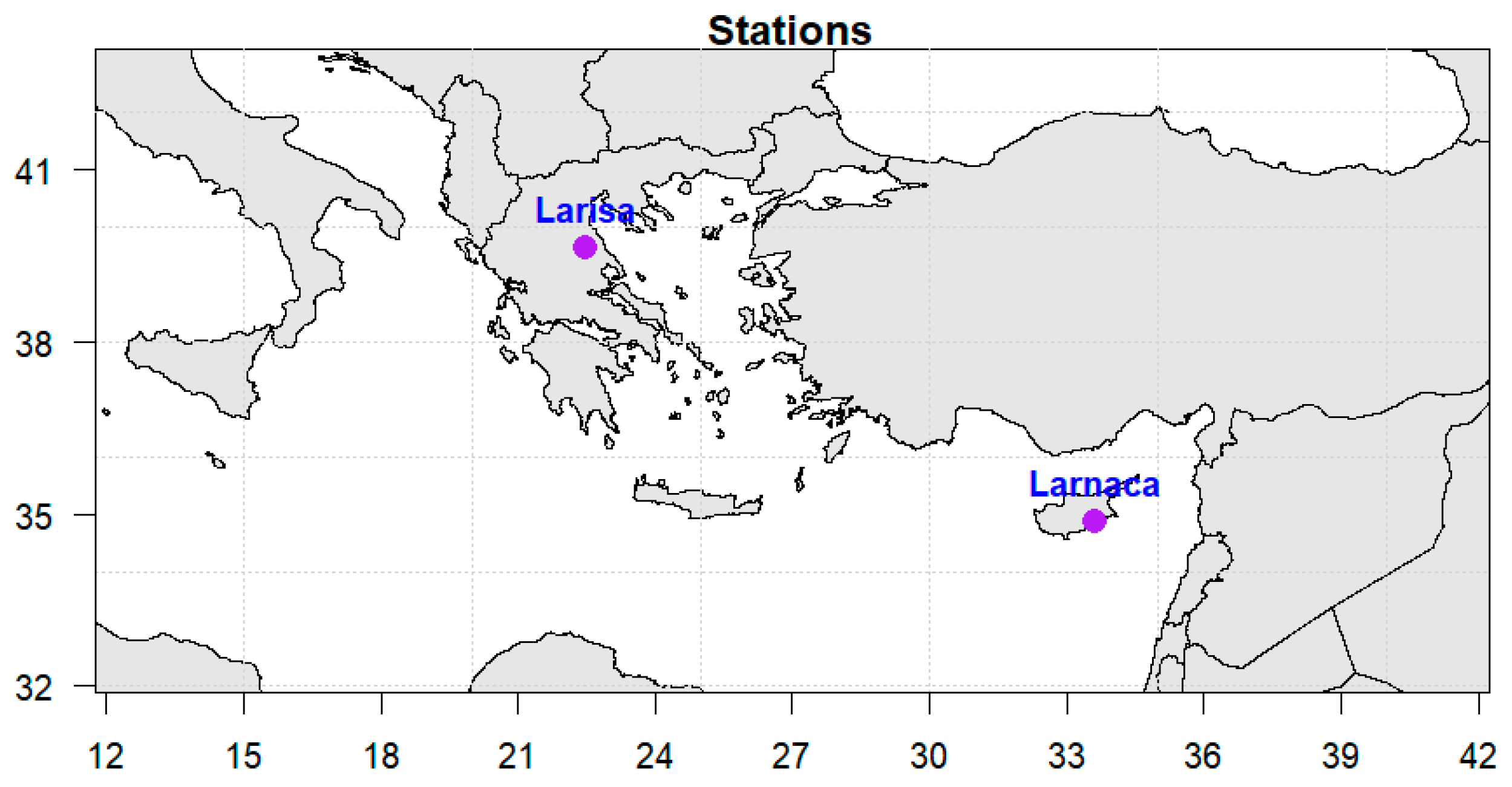
This study used both observed daily precipitation data from ground stations and simulated daily precipitation data from the regional climate model (RCM) during the 25-year period of 1981–2005. The ground station data were obtained from the Global Summary of the Day (GSOD), which provides global coverage of daily meteorological measurements from ground stations and underwent quality control to eliminate errors. Two stations in the eastern Mediterranean, Larissa and Larnaca (Figure 1), were chosen for this study. The observed daily precipitation data had less than 5% missing values, while the RCM-simulated precipitation data were obtained from the regional climate model GERICS-REMO2015 at a spatial resolution of 12.5 km, which was randomly selected from the EURO-CORDEX ensemble. The analysis used the closest continental model grid cell to each station and utilized the Earth System Model version 2G developed by the National Oceanic and Atmospheric Administration’s Geophysical Fluid Dynamics Laboratory (NOAA-GFDL-ESM2G) as the driving global climate model.

2.2. Methodology

The BC approach used follows the steps below:

(1)

The closest continental model grid point was selected for the two studied stations.

(2)

The observed and simulated daily precipitation values were separated into two equal-length sub-periods, the “calibration” and the “evaluation”. Hence, each one of the two sub-periods consisted of 4566, with no temporally coherent precipitation values. For assessing the sensitivity of the proposed method on the selection of the calibration and the evaluation period and equivalently on different climatic conditions, this step was repeated 100 times (bootstrapping).

(3)

The Q-GAM method was applied to the daily rainfall data, and comprised nine steps. Firstly, the proportion of dry days for the observed and modeled data is computed: π_m(c) and π_o(c), as well as the difference π_d = π_o(c) − π_m(c) (with π indicating the proportion). Additionally, the observed rainfall time series were represented by o_t and the RCM model rainfall by m_t, where t is the daily time step and the superscript relates to either the calibration period τ = c or the evaluation period τ = e. A day is defined as “dry” when its total precipitation amount is zero, noting that this can be trivially extended to any value below a certain threshold (e.g., 0.1 mm).

Secondly, all dry days were excluded from observed and modelled data to create a new set of time series. The rainfall values exceeding the 0.99 sample quantile of each time series have been excluded from the analysis. The corrections of such extreme values need a separate analysis. In the next step, we calculated an equidistant sample of quantiles for the observed and modelled time series. This is based on empirical quantile mapping, which avoids the choice of a parametric model to describe the marginal distribution of observed and modelled precipitation.

Following that, it is of high importance to ensure that the GAM captures the relationship between the quantiles of the model data and the non-zero quantiles of the observations. Climate models tend to simulate a smaller number of rainy days, something that holds for the chosen area of study.

In what follows, a brief definition of GAMs is presented. For a deeper understanding of this tool, we propose [9]. A GAM based on the Normal distribution is given with

o_p ~N(f(m_p), σ²)

(1)

f(m_p) = exp{s(m_p)}

(2)

where s(mp) is a smooth function of the model precipitation quantiles, defined by penalized regression splines [9].

This modelling approach estimates the “quantile mapping function” f(m_p) between observed and modelled precipitation quantiles. The choice of distribution (e.g., Normal) is of secondary concern, since the aim here is to estimate f(·). In addition, parameterizing f(·) explicitly allows for extrapolation to unobserved quantile values (the robustness of this assessed in the bootstrapping experiment).

After computing the f(·), the non-zero values were computed for the studied period. Then we calculated the extra number of dry days needed in the corrected values, so that the difference in the proportion of dry days π_d is preserved.

(4)

Finally, the bias corrected values were compared with the corresponding observed ones.

3. Results

To evaluate the efficacy of the Q-GAM method in improving the distribution of the simulated rainfall values, we present a comparison of three data sets for the evaluation period (2000–2005). In particular, a statistical analysis compares the initial simulated daily rainfall amounts with the bias-corrected ones with the Q-GAM method and the observed values. The analysis is presented for the two studied stations (Larissa and Larnaca).

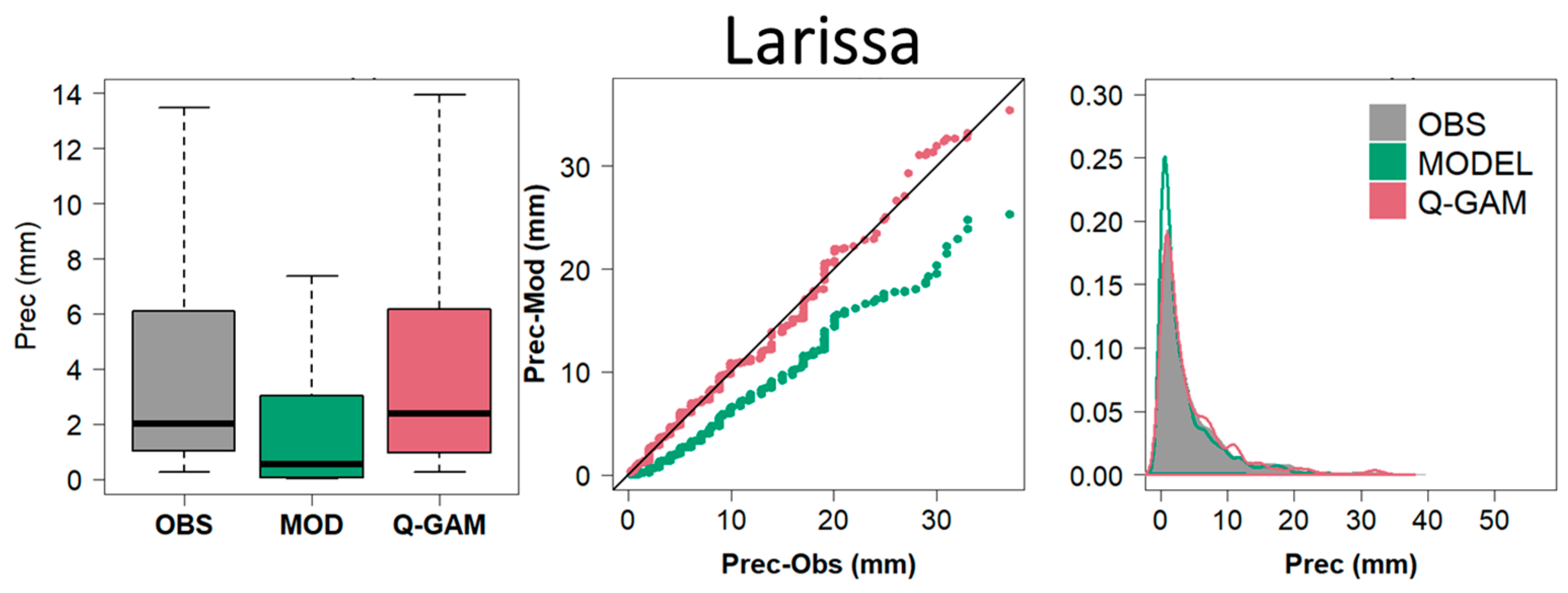
Figure 2 shows three comparison plots for the Larissa station. The first presents the observed (grey), simulated (green), and bias-corrected (pink) daily precipitation values in the form of boxplots. Accordingly, the model underestimates the observed values in all quantiles (e.g., 0.25, 0.50, 0.75, and 1). In contrast, a significant improvement is obtained at all levels after using the Q-GAM method. This outcome is confirmed by the second plot, the Quantile–Quantile plot (QQ). The simulated precipitation amounts diverge from the diagonal respect line, denoting biases between the observed and simulated values. Conversely, the line of the corrected values accurately fits the diagonal one, meaning there is a good match between the two studied time series. The density plot (Figure 2—right panel) shows that the model erroneously simulates a greater frequency of low-precipitation-amount days and underestimates the extreme values, and that both elements are corrected with the Q-GAM method. It should also be mentioned that a significant improvement is recorded in the proportion of dry days. The model simulates that 57% of the studied days have precipitation amounts equal to zero. According to the observations, this percentile is 78%, which is very close to the bias-corrected values (80%).

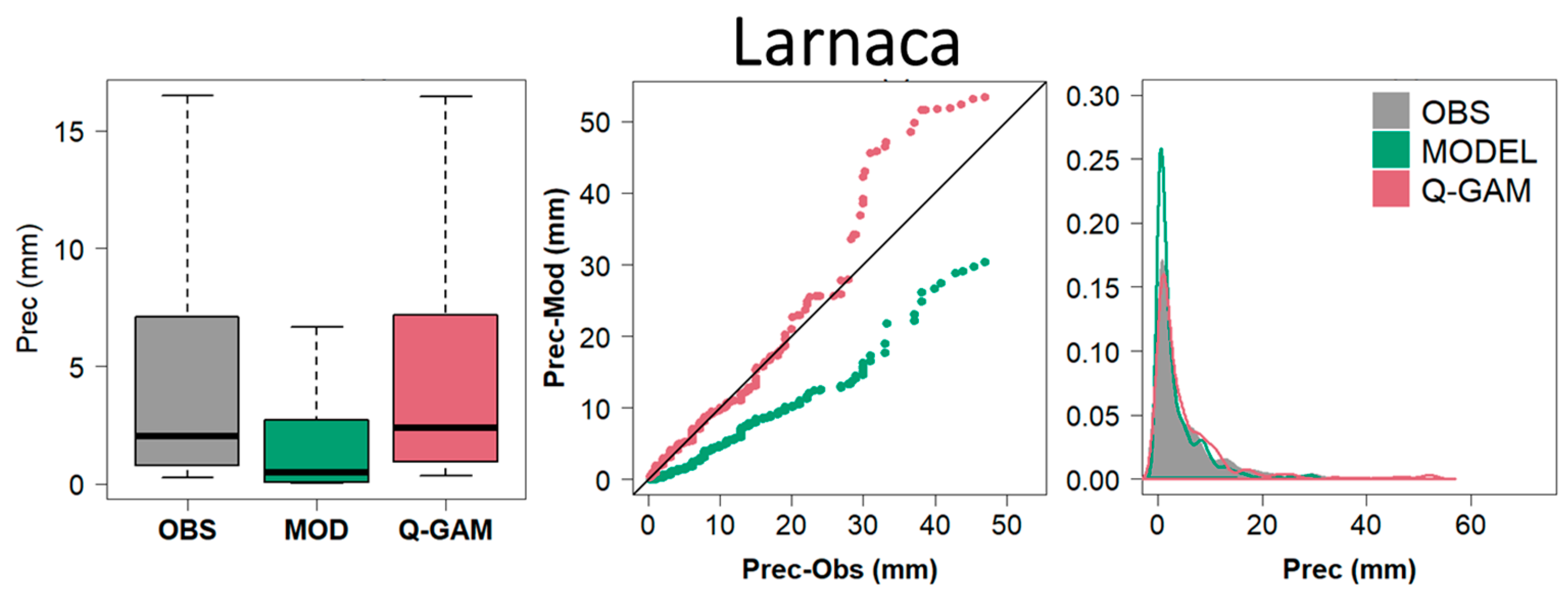
The Larnaca results in Figure 3 show a similar performance. The percentage of dry days is appropriately corrected from 70% to 88%, while the modeled under-prediction is also corrected (as demonstrated by the boxplot). The QQ plot (Figure 3—middle panel) reveals that the bias-corrected values fit very well with the observed ones until about the 0.7 quantile, while for the greatest values, an overestimation is observed. The density plot shows a significant improvement in the frequency of the lowest precipitation amounts (Figure 3—right panel).

Table 1. Proportion of times in the bootstrapping experiment when the bias-corrected data outperformed the initial climate model output, for each station. Statistics other than the proportion of zeros are computed for non-zero days.

Station	Proportion of Zeros	Annual Sum	90%	95%	Mean	Standard Deviation
Larissa	100	87	96	95	98	82
Larnaca	100	71	99	91	99	92

presents a frequency analysis of the results obtained from the bootstrapping loop for each station, which quantifies the degree of improvement achieved. Examining the aggregate performance of the Q-GAM method across multiple runs provides insight into its robustness to various factors, including (a) climate conditions at each station, (b) temporal variability in climatological conditions, and (c) variability in the accuracy of the RCM. The table indicates the proportion of times that the Q-GAM correction method outperformed the original model output for each of the six summary statistics, thereby highlighting the success of the method. To determine success, the difference between the observations and (a) the RCM data and (b) the corrected RCM data was calculated for all metrics. If the difference for the corrected data was smaller than the RCM data, it was considered a success. Table 1 displays the percentage of such successes. The results show that the proportion of dry days is improved across all stations, regardless of the evaluation and calibration period. The total annual precipitation is also improved across almost all runs, indicating that the method is robust to the choice of the calibration and evaluation period, as well as the station’s climatology.

To evaluate the Q-GAM method’s ability to correct precipitation extremes, we analyzed its performance using the 90% and 95% percentiles. Our results, as shown in Table 1, demonstrate that the method significantly reduces the biases between the observed and corrected data in at least 90% of the runs for both percentiles. We also assessed the mean and standard deviation of the precipitation distribution (Table 1), which indicates a significant improvement in these statistics. Specifically, the standard deviation improves in a minimum of 75% of the runs, highlighting the effectiveness of the Q-GAM method in correcting precipitation extremes.

4. Discussion and Conclusions

We present a new method, called the Q-GAM method, which combines quantile mapping and generalized additive models (GAMs) for bias correction. The method is adaptable and flexible, as the quantiles of both model output and observations are calculated empirically, and mapping is performed using penalized non-linear regression. We applied the method to the data from two eastern Mediterranean stations (Larissa and Larnaca) and evaluated its performance. We also demonstrate the method’s robustness using a bootstrapping experiment, which considers the station’s location (climate characteristics) and temporal variability, both of which are known to affect bias correction performance [10,11]. The data were split into calibration and evaluation periods, and we varied these periods in the bootstrapping experiment. Our results indicate that the Q-GAM method performs well across various calibration/evaluation periods, with over 70% of the runs for most metrics in both stations showing bias-corrected time series statistics that are closer to the observed data. This gives us confidence in applying the Q-GAM method to future climate projection data, even when the climate conditions may be different.

Our investigation shows that the Q-GAM approach is a robust and accurate method for the bias correction of daily precipitation, with the added advantage of low computational cost. The Q-GAM method was also found to significantly improve the number of dry days and high rainfall extremes while replicating the precipitation regime of the two regions well. Traditional bias correction methods often fail to detect dry days, but this is not an issue with the Q-GAM method.

Although this work is exploratory, it provides valuable insights into using GAMs with quantile mapping for bias correction. The use of GAMs allows for the inclusion of more than one model variable in the correction, such as temperature or pressure, through a multi-variable transfer function defined by tensor product interaction. Additionally, station-specific variables like spatial coordinates or elevation can be added to the transfer function as an interaction term and applied simultaneously to multiple locations, which is a critical element in bias-correcting model output in the absence of observations. These further developments will be explored in future work.

References

- Maraun, D.; Widmann, M. Statistical Downscaling and Bias Correction for Climate Research; Cambridge University Press: Cambridge, UK, 2018. [Google Scholar] [CrossRef]
- Christensen, J.H.; Boberg, F.; Christensen, O.B.; Lucas-Picher, P. On the need for bias correction of regional climate change projections of temperature and precipitation. Geophys. Res. Lett. 2008, 35, L20709. [Google Scholar] [CrossRef]
- Maraun, D. Bias correcting climate change simulations-a critical review. Curr. Clim. Chang. Rep. 2016, 2, 211–220. [Google Scholar] [CrossRef]
- Goodison, B.E.; Louie, P.Y.; Yang, D. Wmo Solid Precipitation Measurement Intercomparison; World Meteorological Organization: Geneva, Switzerland, 1998. [Google Scholar]
- Vrac, M.; Noel, T.; Vautard, R. Bias correction of precipitation through singularity stochastic removal: Because occurrences matter. J. Geophys. Res. Atmos. 2016, 121, 5237–5258. [Google Scholar] [CrossRef]
- Hagemann, S.; Chen, C.; Haerter, J.O.; Heinke, J.; Gerten, D.; Piani, C. Impact of a statistical bias correction on the projected hydrological changes obtained from three gcms and two hydrology models. J. Hydrometeorol. 2011, 12, 556–578. [Google Scholar] [CrossRef]
- Piani, C.; Haerter, J.O. Two dimensional bias correction of temperature and precipitation copulas in climate models. Geophys. Res. Lett. 2012, 39, L20401. [Google Scholar] [CrossRef]
- Lazoglou, G.; Angnostopoulou, C.; Tolika, K.; Benedikt, G. Evaluation of a New Statistical Method—TIN-Copula–for the Bias Correction of Climate Models’ Extreme Parameters. Atmosphere 2020, 11, 243. [Google Scholar] [CrossRef]
- Wood, S. Generalized Additive Models: An Introduction with r, 2nd ed.; Chapman and Hall/CRC: Boca Raton, FL, USA, 2017. [Google Scholar]
- Chen, J.; Brissette, F.P.; Chaumont, D.; Braun, M. Finding appropriate bias correction methods in downscaling precipitation for hydrologic impact studies over north America. Water Resour. Res. 2013, 49, 4187–4205. [Google Scholar] [CrossRef]
- Beyer, R.; Krapp, M.; Manica, A. An empirical evaluation of bias correction methods for palaeoclimate simulations. Clim. Past 2020, 16, 1493–1508. [Google Scholar] [CrossRef]