Proceeding Paper

Daily Streamflow Modelling Using ML Based on Discharge and Rainfall Time Series in the Besós River Basin, Spain †

1
Sustainable Water Management and Governance in Natural and Agricultural Environments, Mediterranean Agronomic Institute of Zaragoza (IAMZ), International Centre for Advanced Mediterranean Agronomic Studies (CIHEAM), Av. Montañana 1005, 50059 Zaragoza, Spain
2
Eurecat, Technology Centre of Catalonia, Unit of Applied Artificial Intelligence, 08005 Barcelona, Spain
*
Author to whom correspondence should be addressed.
Presented at the 7th International Electronic Conference on Water Sciences, 15–30 March 2023; Available online: https://ecws-7.sciforum.net.
Environ. Sci. Proc. 2023, 25(1), 30; https://doi.org/10.3390/ECWS-7-14168
Published: 14 March 2023
(This article belongs to the Proceedings of The 7th International Electronic Conference on Water Sciences)

Abstract

:
Machine learning (ML)-based data-driven modelling is an efficient approach for good estimates of flow and maximum discharge at certain points within a basin. This paper is mainly aimed at evaluating the predictive capability of ML algorithms for daily streamflow modelling in the Besós River Basin (Spain), based on open source flow discharge and rainfall historical time series. In this sense, two modelling scenarios, without and with consideration of the antecedent hydrologic conditions, were evaluated, and three ML algorithms—support vector machines, random forest (RF) and gradient boosting (GB)—were compared to multiple linear regression (MLR), and were implemented. The prediction results revealed that the SVR model outperformed the other suggested models. Additionally, it was deduced that taking into account preceding hydrologic conditions clearly improves prediction results.

1. Introduction

Rainfall–runoff modelling is believed to be complex, nonlinear, and time-varying because the basin response depends not only on hydrometeorological parameters but also on spatiotemporal irregularity in basin characteristics and rainfall patterns [1]. Usually, hydrologists develop and use different types of models to simulate hydrological processes. Regardless of their structural variations, these models generally fall into three main types, including physical, conceptual, and data-driven models (DDMs) [2].
Over the past two decades, data-driven approaches based on artificial intelligence (AI), have gained drastically increasing interest from hydrologists [3], due to their significant contribution to improving the accuracy, versus the failure stories, of the classical and conventional methods in terms of spatial scale, time scale, the amount of data needed, facilities, the inability to handle nonlinear and nonstationary hydrological processes, and even in terms of accuracy, viewing the complexity of the equations governing the hydrological cycle’s mechanisms which often require simplifications and theoretical assumptions leading to considerable errors and uncertainties [4].
Many different statistical methods, such as multiple linear regression (MLR), and various types of AI and machine learning (ML) algorithms such as support vector machines (SVM) and artificial neural networks (ANN), have been widely applied in recent years [5]. Especially, ANN and SVM have the advantage of handling complex relationships between input and output variables and have been used successfully in various water resources problems [6]. However, despite the application of several ML techniques available in the literature, the gradient boosting (GB) approach has not been widely applied to predict daily flows [7]. Also, for hydrological extremes, GB and random forest (RF) are more often explored for qualitative predictions rather than quantitative predictions [4].
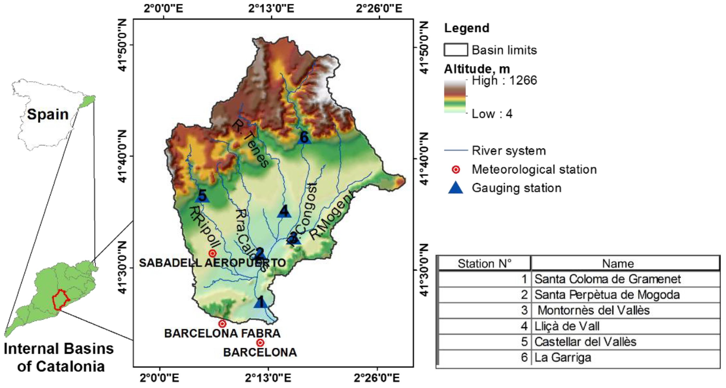
In this sense, this paper presents the application of three regression ML algorithms—support vector regression, random forest regression and gradient boosting regression—were compared to MLR and used to model the daily flow discharge at the outlet of the Besós River basin (Spain) under two scenarios: without and with consideration of the antecedent hydrologic conditions. The objective is to discuss and evaluate the performance of the aforementioned DDMs in daily streamflow prediction based on open-source flow discharge and rainfall historical time series by comparing them with each other and with the MLR model based on several statistical evaluation measures, and to evaluate the impact of using the preceding hydrologic conditions.

2. Materials and Methods

2.1. Study Location and Data Collection

The Besós is a Mediterranean river characterised by a very irregular hydrological regime with highly variable flows related to climatic conditions. It is the collector of various tributaries that originate in the Catalan pre-coastal range, which includes the Mogent, Congost, Tenes, Caldes and Ripoll rivers, as shown in Figure 1. Its hydrographic basin of approximately 1020 km² supports a population of almost one million inhabitants with high water consumption, mainly destined for industrial and urban use, since agriculture, especially in its lower section, has been losing importance, and is close to disappearing. The Besós basin shows a pronounced relief formed by the coastal and precoastal ranges with elevations of up to 1350 m a.s.l. and steep slopes. As indicated by the topography, the geology of the area differs between the mountain ranges, composed mainly of granites, slate, limestone and sandstone, and the central valley where clay, sand, and conglomerate deposits dominate.
In this study, open-source historical series of daily flow and rainfall data between 2003 and 2010 from the Catalan Water Agency and the State Meteorological Agency were gathered. Information was collected on a total of five gauging stations, “La Garriga”, “Castellar Valles”, “Lliçà de Vall”, “Montornès Valles”, and “Santa Perpetua de Mogoda”, and three meteorological stations, “Barcelona”, “Barcelona Fabra” and “Sabadell Aeropuerto”, were used to explore the applicability of ML models for daily flow discharge prediction at the target station “Santa Coloma de Gramenet”. Figure 1 shows the geographical distribution of the stations.

2.2. Exploratory Analysis and Data Preparation

2.2.1. Data Exploration

The available collected data are distributed over a period from 1 January 2003 to 31 December 2010, as some stations no longer have records after this date. The longest common period with the fewest missing values is from 1 January 2003 to 6 May 2008. Therefore, this observation period was considered in creating the prediction models.
For this common period, the “Castellar del Vallès” gauging station has a considerable number of missing values (about 56.18%), so it was decided that it would not be considered in the modelling process, and the lost information could be therefore obtained from the “Sabadell Aeropuerto” meteorological station. Also, the meteorological stations and the “La Garriga” gauging station presented some missing values in their data series (<16%). For that reason, because data imputation may lead to additional uncertainties to those series due to measurement errors, it was decided that all data rows for which at least one station had a missing value were deleted, and that the models would learn from the rest of the data that were supposed to be sufficient for their training and validation. The resulting data time series contained a total of 1404 daily rainfall and flow records.
The basic information of the observatories and the dataset statistical analysis conducted after dealing with the missing values showed that the Besós basin receives, in its lower part, as represented by the “Sabadell Aeropuerto” station, an average annual rainfall of 415 mm varying from 0 to 122 mm per day. The average flow discharge at its outlet (“Santa Coloma del Vallès”) is 4.4 m3/s, and most flow values are below 20 m3/s. Only two values exceeded 80 m3/s during this observation period. Also, the flow discharge has never been zero.
The parameters “skewness” and “kurtosis” were used to examine the data distribution. Practically, all the data time series have very large values of these coefficients and therefore do not have a normal distribution.
A correlation heat map was created to explore the relationship between the different data inputs, showing a good correlation between meteorological stations (rainfall) as well as between gauging stations (flow), while no correlation was detected between flow and rainfall, reflecting the nonlinear rainfall–flow relationship.

2.2.2. Data Model

The selection of input variables is determined by a combination of prior knowledge of causality, examination of time series plots, data availability, and study objectives. In this study, we used rainfall and flow discharge data, with rainfall being the primary driving force of runoff. Since only one meteorological station was located within the basin, we utilized data from two neighbouring stations outside the basin (as shown in Figure 1) to define the rainfall in the differential basin between upstream gauging stations and the prediction point (target station).
Given that flow is effectively made up of contributions from different subareas whose travel time covers a range of values, the next step was the determination of the appropriate lag time concerning the prediction output. This was carried out through a cross-correlation analysis between the flow at the outlet and the upstream and downstream rainfall and flow. The cross-correlation showed the considerable influence of the previous day’s (t−1) rainfall on the current value of the outlet flow for the three meteorological stations. From time t−2, this correlation decreased to less than 0.3. Also, regarding the flow at the input stations, it was seen that there was a decreasing correlation from the same day of recording. The antecedent flow subsequent to time instant t−2 did not contribute significantly to the outflow generation. Therefore, the antecedent values of flow and rainfall corresponding to time instants t and t−1 were considered.
When looking at the time step, several features are immediately obvious, such as the day of the month and the month of the year, which may be helpful in understanding the flow periodicity or seasonality. It is then necessary to use variables that extract and preserve hidden information within cyclical data, such as the distance between two events: day 30 or 31 and day 1, or month 12 and month 1. This seems important as the missing values were removed. To do this, “sin” and “cos” were used to assign each cyclic variable (day and month) to a circle so that the smallest value for that variable appeared right next to the largest value. Four cyclic features (daysin, daycos, monthsin, and monthcos) with respect to the day and the month of the year were created to obtain a total of 18 input features.
The general representative DDM for the first scenario can be defined as:
Q^t = f(Qit, Qit−1, Pkt, Pkt−1, daysin, daycos, monthsin, monthcos)
where Q^t represents the predicted flow at time t at the “Santa Coloma de Gramenet” station; Qit is the flow recorded at time t at each of the predictor gauging stations; Qit−1 is the flow recorded at these gauging stations at time t − 1 (‘i’ ranges from 1 to 4); Pkt represents the rainfall at time t observed at each of the meteorological stations; Pkt−1 is the rainfall at time t − 1 observed at each of the meteorological stations (‘k’ ranges from 1 to 3); and daysin, daycos, monthsin, and monthcos represent the features or cyclical variables of the day and month.
These variables were used to predict the flow at the “Santa Coloma de Gramenet” station as a first scenario, which was intended to be extrapolated to basins without a gauging station or flow measurement, depending on their physiographic characteristics and climatic conditions. In the second scenario, in addition to these input variables, the antecedent flow discharge of the “Santa Coloma de Gramenet” station was also used as an input variable, since it indirectly describes the soil moisture status. Also, since the rainfall data contain zero values, such flows add more information, meaning that the longer the zero-input interval, the more the output decreases. The above was conducted by performing an autocorrelation for the target variable dataset, between the previous values and the current one up to 5 lags. In this second scenario, DDMs could be used in poorly gauged or previously gauged catchments where flow measurements were interrupted or as a virtual sensor for the Besós river basin itself. The autocorrelation showed the considerable influence of the two previous values (correlation ≥ 0.4). Therefore, the antecedent flows at the target station at times t − 1 and t − 2 were considered. This was also verified by trial and error experiments.
The general representative DDM, in this second scenario, can be defined as:
Q^t = f(Qit, Qit−1, Pkt, Pkt−1, Qot−1, Qot−2, daysin, daycos, monthsin, monthcos)
where Qot−1 and Qot−2 are the antecedent flows at times t − 1 and t − 2 observed at the “Santa Coloma de Gramenet” outlet gauging station.
To prevent input data in larger numerical ranges from dominating those in smaller numerical ranges and to avoid numerical difficulties during computation, all input variables were scaled to the range [0, 1] using the Min-Max Scaler method. The complete chronologically organized dataset was then divided into training and test datasets to obtain an approximate training/test split ratio of 80%/20%.

2.2.3. Hyperparameter Optimisation

Models were trained with a range of hyperparameter values that was determined by examining various hydrological studies. Afterwards, the hyperparameter optimal values were determined through a trial and error process using the Grid Search technique due to its simplicity and robustness, in the training and test datasets. Then, the optimal hyperparameters were maintained and the best models were used to predict the flow rate.

2.2.4. Validation Metrics

Four quantitative validation metrics, including: the coefficient of determination (R²), the Nash–Sutcliffe efficiency coefficient (NSE), the Mean Absolute Error (MAE) and the Root Mean Squared Error (RMSE), were used to assess the prediction accuracy and to compare the different data-driven models based on their relative performance.

3. Results and Discussion

The values of the DDM-statistical performance metrics for the training and test periods are presented in Table 1. Hydrographs were also plotted to visualize the DDM behaviour, particularly for extreme values.
It is clear from Table 1 that the RFR and GBR models were more efficient in predicting the flow for the first scenario, in the training period, with a slight victory for the RFR model, reaching R2 values of 0.945 and 0.936, respectively; RMSEs of 0.983 m3/s and 1.062 m3/s; MAEs of 0.259 m3/s and 0.558 m3/s, and approximately equal NSEs. However, the SVR outperformed all models in the test period for all metrics.
MLR performance was not as good as that of the three other DDMs, but it was very acceptable concerning performance metrics. It outperformed the RF model in the test period with respect to the MAE and the SVR model in the training period regarding the NSE. The fact that the MLR prediction values have a good correlation with the observed values is related to the fact that the number of input gauging stations was slightly higher than that of meteorological stations, that the flow discharge values had more weight in the MLR equation than those for rainfall, and that the flow inputs showed a good linear correlation with each other, unlike the rainfall inputs.
Interestingly, the prediction results are satisfactory, and there are some improvements in the performance of the models in the test period compared to the training period, except for GBR regarding the R² and NSE and RFR regarding the MAE, R² and NSE. This may have been the result of overfitting these models.
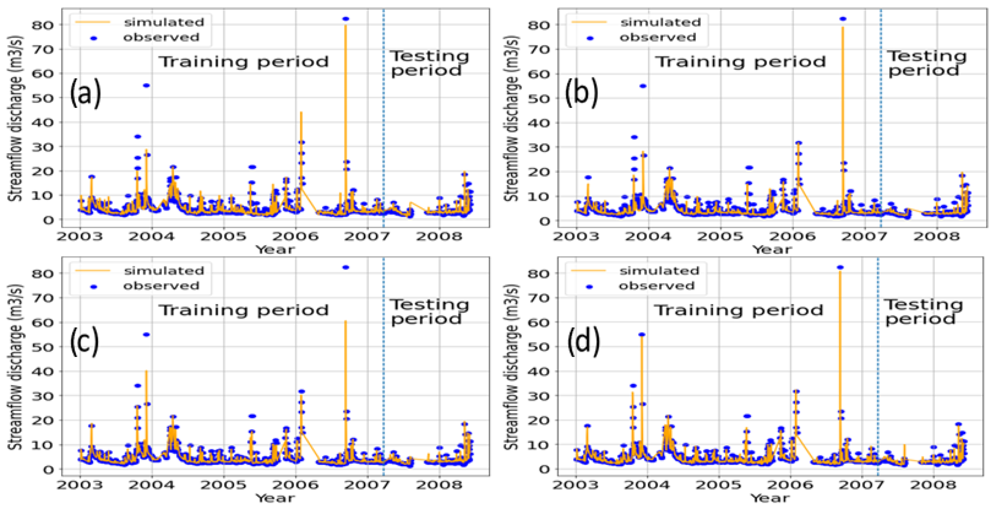
The hydrographs in Figure 2 and Figure 3 of the observed and predicted values for each model in the training period, as well as the test period at the target station, indicate that, in general, the predicted flow fits well with the observed flow.
However, for the training period, it can be seen that there were more peaks than there were in the test period. The maximum peak observed in the training period was underestimated by all the models, but it can be seen that MLR, SVR and GBR managed to approximate it well, while RFR presented a high relative error at this point. In general, the RFR had the best performance in the training period.
Possible reasons for this result could be the better generalisation ability of SVR due to the structural risk minimisation approach which led to an optimal global solution. Regarding the overfitting of the GBR and the RFR models, it should first be remembered that these two models are based on building trees from a random Bootstrap sample, which makes both models stochastic, with an uncertainty associated with the predicted value. The high number of trees that was found to have trained the two models may have been behind this overfitting. Also, GBR is a nondeterministic algorithm; i.e., even for the same input, it can present different outputs in different executions.
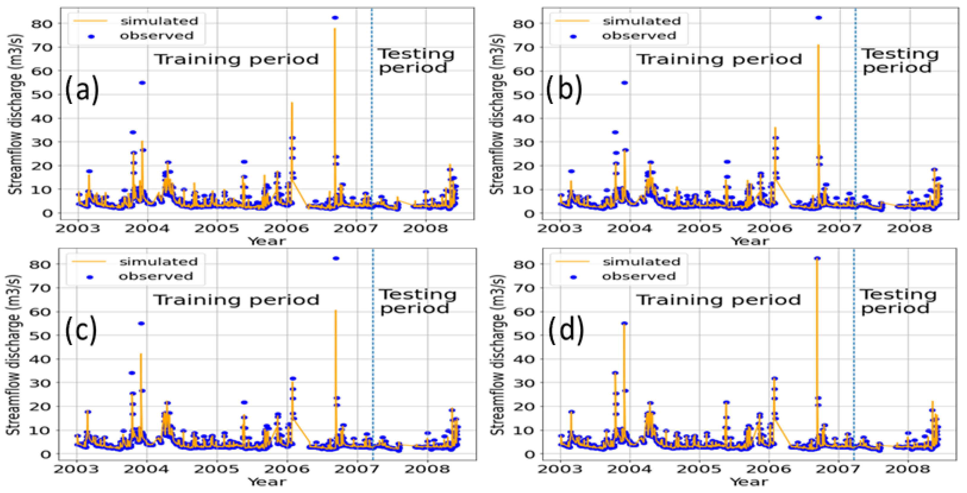
Regarding the second scenario, the GBR outperformed all models in the training period with near-perfect performance. In the test period, the SVR in this case was also the best regarding all metrics.
Some DDM performance improvements were shown in the test period compared to the training period. Regarding SVR, all metrics improved. For MLR, only RMSE and MAE improved. In contrast, the GBR and the RFR showed a decrease in their performance, except for the RMSE of the RFR, which improved. This overfitting, in addition to the aforementioned reasons, may have been due to the insufficient data size, or that the data’s split ratio for training and testing the models was not adequate. Generally, the simulated hydrographs fit well with the observed hydrographs. It is seen that GBR has a great ability to predict flow peaks. All models predicted the flow at the basin outlet well.
When comparing the DDMs, it can be seen that the use of the antecedent flow discharges had a great impact in improving their performance, with a reduction in the MAEs of 23%, 17%, 21% and 33% for the MLR, SVR, GBR and RFR models. The RFR showed the greatest improvement in performance during the test period with a decrease in the RMSE and MAE of 18% and 33%, and an increase in the R² and NSE of 6% and 7%, respectively.

4. Conclusions

To predict the daily flow at the outlet of the Besós river basin, the MLR and three data-driven ML models, SVR, RFR and GBR, were used. The obtained results show that the SVR model outperformed the other models whether or not the preceding hydrologic conditions were considered. MLR, as well as the decision tree ensemble models (RFR and GBR), has also shown a good flow prediction capacity. It is worth noting that the proposed DDMs have demonstrated high efficiency in capturing the real trend and the underlying phenomena of rising and falling flow curves. The use of the antecedent flows in the target gauging station had a positive impact on improving the performance of all models.
To improve the prediction capabilities of ML models, in future work, it is recommended to use other variables to build a strong relationship with the streamflow; to perform a sensitivity analysis of input features to bring out those that contribute the most to the flow prediction; to pay close attention to the data length and split ratio; to ensure that the training phase experiences most of the streamflow patterns to allow the models in the test period to simulate the flow discharge with an acceptable level of accuracy.

Author Contributions

M.H. and M.R. conceived, designed, and led the research and contributed to the paper editing; M.H. was behind the research conceptualisation and analytical development. M.R. supervised all actions. All authors have read and agreed to the published version of the manuscript.

Funding

This research was funded by the International Centre for Advanced Mediterranean Agronomic Studies (CIHEAM).

Institutional Review Board Statement

Not applicable.

Informed Consent Statement

Not applicable.

Data Availability Statement

The data, programming codes and additional material were uploaded to: https://www.kaggle.com/datasets/mohamedhamitouche/rainfall-and-runoff-data-for-the-bess-river-basin (accessed on 10 March 2023).

Conflicts of Interest

The authors declare no conflict of interest.

References

  1. Cheng, K.; Wei, S.; Fu, Q.; Pei, W.; Li, T. Adaptive management of water resources based on an advanced entropy method to quantify agent information. J. Hydroinform. 2019, 21, 381–396. [Google Scholar] [CrossRef]
  2. Zhang, L.; Yang, X. Applying a multi-model ensemble method for long-term runoff prediction under climate change scenarios for the Yellow River Basin, China. Water 2018, 10, 301. [Google Scholar] [CrossRef]
  3. Terzi, Ö.; Ergin, G. Forecasting of monthly river flow with autoregressive modeling and data-driven techniques. Neural Comput. Appl. 2014, 25, 179–188. [Google Scholar] [CrossRef]
  4. Hamitouche, M.; Molina, J.L. A Review of AI Methods for the Prediction of High-Flow Extremal Hydrology. Water Resour. Manag. 2022, 36, 3859–3876. [Google Scholar] [CrossRef]
  5. Isunju, J.B.; Kemp, J. Spatiotemporal analysis of encroachment on wetlands: A case of Nakivubo wetland in Kampala, Uganda. Environ. Monit. Assess. 2016, 188, 203. [Google Scholar] [CrossRef] [PubMed]
  6. Hosseini, S.M.; Mahjouri, N. Developing a fuzzy neural network-based support vector regression (FNN-SVR) for regionalizing nitrate concentration in groundwater. Environ. Monit. Assess. 2014, 186, 3685–3699. [Google Scholar] [CrossRef] [PubMed]
  7. Fonseca, T.L.; Gorodetskaya, Y.; Tavares, G.G.; de Melo Ribeiro, C.B.; da Fonseca, L.G. A Gradient Boosting Model Optimized by a Genetic Algorithm for Short-term Riverflow Forecast. Rev. Mundi Eng. Tecnol. Gestão 2019, 4, 3845. [Google Scholar] [CrossRef]
Figure 1. Study area and location of the meteorological and gauging stations.
Environsciproc 25 00030 g001
Figure 2. First scenario’s hydrographs of the observed and simulated flow discharge in the training and test periods. (a) MLR, (b) SVR, (c) RFR, and (d) GBR.
Environsciproc 25 00030 g002
Figure 3. Second scenario’s hydrographs of the observed and simulated flow discharge in the training and test periods. (a) MLR, (b) SVR, (c) RFR, and (d) GBR.
Environsciproc 25 00030 g003
Table 1. Model performance metrics for training and test periods.
ScenarioModelTrainingTest
RMSEMAENSERMSEMAENSE
1MLR1.7830.7800.8190.7790.8060.5020.8190.808
SVR1.6850.6000.8380.7740.6040.3690.8980.877
GBR1.0620.5580.9360.9280.7200.4800.8560.844
RFR0.9830.2590.9450.9220.7580.5450.8400.834
2MLR1.4770.5830.8760.8580.7760.3880.8330.850
SVR1.5630.4920.8610.8050.5780.3070.9070.890
GBR0.1710.1310.9980.9980.6850.3810.8690.862
RFR0.9210.2070.9520.9330.6240.3680.8920.890
Disclaimer/Publisher’s Note: The statements, opinions and data contained in all publications are solely those of the individual author(s) and contributor(s) and not of MDPI and/or the editor(s). MDPI and/or the editor(s) disclaim responsibility for any injury to people or property resulting from any ideas, methods, instructions or products referred to in the content.

